Article

Complementary Relationship-Based Validation and Analysis of Evapotranspiration in the Permafrost Region of the Qinghai–Tibetan Plateau

1
School of Hydrology and Water Resources, Nanjing University of Information Science and Technology, Nanjing 210044, China
2
Northwest Institute of Eco-Environment and Resources, Chinese Academy of Sciences, Lanzhou 730000, China
*
Author to whom correspondence should be addressed.
Atmosphere 2025, 16(8), 932; https://doi.org/10.3390/atmos16080932
Submission received: 17 June 2025 / Revised: 19 July 2025 / Accepted: 31 July 2025 / Published: 1 August 2025
(This article belongs to the Section Meteorology)

Abstract

The Complementary Relationship (CR) principle of evapotranspiration provides an efficient approach for estimating actual evapotranspiration (ETa), owing to its simplified computation and effectiveness in utilizing meteorological factors. Accurate estimation of actual evapotranspiration (ETa) is crucial for understanding surface energy and water cycles, especially in permafrost regions. This study aims to evaluate the applicability of two Complementary Relationship (CR)-based methods—Bouchet’s in 1963 and Brutsaert’s in 2015—for estimating ETa on the Qinghai–Tibetan Plateau (QTP), using observations from Eddy Covariance (EC) systems. The potential evapotranspiration (ETp) was calculated using the Penman equation with two wind functions: the Rome wind function and the Monin–Obukhov Similarity Theory (MOST). The comparison revealed that Bouchet’s method underestimated ETa during frozen soil periods and overestimated it during thawed periods. In contrast, Brutsaert’s method combined with the MOST yielded the lowest RMSE values (0.67–0.70 mm/day) and the highest correlation coefficients (r > 0.85), indicating superior performance. Sensitivity analysis showed that net radiation (Rn) had the strongest influence on ETa, with a daily sensitivity coefficient of up to 1.35. This study highlights the improved accuracy and reliability of Brutsaert’s CR method in cold alpine environments, underscoring the importance of considering freeze–thaw dynamics in ET modeling. Future research should incorporate seasonal calibration of key parameters (e.g., ε) to further reduce uncertainty.

1. Introduction

Evapotranspiration (ETa) is an important component of the water and energy budget of the land surface in the hydrological cycle and climate change [1,2]. Accurate estimation of ETa to model terrestrial hydrological and ecological processes is necessary. The ETa of the Qinghai–Tibetan Plateau (QTP) is the largest permafrost region in the mid–high latitudes, often referred to as the “Asian Water Tower,” and plays a crucial role in the global water cycle and has attracted considerable global attention [3]. The reliable estimation of ETa is crucial for understanding the hydrothermal balance on the QTP [4,5].
At present, several established measurement techniques are commonly employed to obtain an accurate ETa, such as weighing lysimeters, the Eddy Covariance (EC) system, the Bowen ratio tower, and large aperture scintillometers [6]. However, the existing sparse observations make it difficult to meet the data requirements for studying the spatiotemporal distribution of ETa in the cold climate environment over the QTP. Therefore, several mathematical models were developed to estimate ETa in recent years [7,8]. The Penman–Monteith method is well known for calculating ETa, which was improved by Monteith introducing the resistance parameter into the Penman equation [9,10]. Based on this, Mu et al. [11] developed a global remote-sensing evapotranspiration algorithm. However, due to the uncertainty of the aerodynamic and surface resistance, it remains challenging to achieve high accuracy in ETa estimation on the QTP. In addition, ETa can be estimated based on the surface energy balance, such as SEBAL and SEBS [12]. The models were applied to estimate ETa over the QTP [13,14,15]. It was found that the ETa was overestimated in winter on the QTP, which was caused by the questioning of the parametric scheme [16,17,18].
The Complementary Relationship (CR) principle is another effective method to estimate ETa [19,20]. The first complementary concept of evapotranspiration was proposed by Bouchet [21] in general terms. The potential evapotranspiration (ETp) and ETa are strongly coupled through land and atmospheric feedback [22]. When there is a limitation in energy without having a limitation in water availability, the wet environment evapotranspiration (ETw) is introduced, and it can be expressed as ETa = ETw = ETp. As the water availability decreases, ETa decreases, whereas ETp increases. Numerous studies have reported a decreasing ETp over large areas in different regions over the past 50 years, and this contrasts with the reports of increasing ETa [23,24,25]. They were regarded as a symmetrical relationship (ETa < ETw < ETp), so it could be expressed with a linear equation at first. But in fact, the relationship is asymmetric in the natural environment. Thus, several models were developed to explain the complementary relationship of evapotranspiration from the natural land surface based on the original concept, which included the complementary relationship areal evapotranspiration model [26], the advection–aridity model [27], the Granger and Gray model [28], and the nonlinear complementary functions. These methods have been widely utilized to estimate ETa due to their simple calculation without requiring complex parameters. Brutsaert et al. [29,30] proposed the nonlinear complementary relationship principle based on physical considerations. It was demonstrated that the nonlinear function performed better under semi-arid conditions.
ETa is expected to have various trends at different temporal scales, attributed mainly to the variability in the climate system [31,32,33]. A large number of studies have focused on the variation in and attribution of ETa in different regions [34,35,36]. Sensitivity and multiple regression analyses are the most commonly used methods for quantifying the contributions of the driving factors to ETa. Talsma et al. [37] analyzed the sensitivity of remote sensing-based models on the uncertainty of the input variables and found that the models were most sensitive to the Normalized Difference Vegetation Index (NDVI), relative humidity, and net radiation. Cawse-Nicholson et al. [38] found the disaggregated atmosphere–land exchange is most sensitive to the land surface temperature.
The QTP is extremely sensitive to climate change, with observed increases in air temperature and changes in snow cover, soil moisture, and permafrost extent [39,40,41]. These environmental changes have significant implications for evapotranspiration processes, which are closely linked to the surface energy balance and water cycling over frozen and thawed ground conditions. Despite its importance, ETa remains poorly constrained over permafrost regions due to challenges in measurement and modeling, especially under freeze–thaw transitions [42,43]. Therefore, improving ETa estimation in permafrost-dominated areas is essential for understanding land–atmosphere interactions and predicting water and energy fluxes under future climate scenarios. This study aims to address this gap by applying and validating CR approaches over three representative permafrost sites on the QTP.
In this study, we conducted a comprehensive analysis of ETa on the QTP. The observed ETa, obtained through the EC system, was juxtaposed with the calculated ET to examine the validity of the complementary relationship. This comparison was carried out at three distinct meteorological stations located across the QTP. Subsequently, we delved into the impact and attribution of climate change on ETa. This investigation was particularly focused on understanding the influence of the freeze–thaw cycle prevalent on the QTP. Our findings contribute to the growing body of knowledge on the intricate interplay between climate change and evapotranspiration patterns, thereby offering valuable insights for future research and policymaking.
Overall, the primary objective of this study is to evaluate the applicability and performance of two CR approaches—Bouchet’s [21] and Brutsaert’s [29] methods—for estimating ETa in the permafrost region of the QTP. Specifically, the study aims to (1) validate the CR between ETa and ETp using observed ETa from EC systems; (2) assess the influence of different wind functions, including the Monin–Obukhov Similarity Theory (MOST) and the Rome wind function, on ETp calculations via the Penman equation; and (3) analyze the sensitivity and contribution of meteorological factors to ETa under freeze–thaw conditions. A key goal is to determine the suitability and limitations of each CR method during the soil-frozen and soil-thawed periods in a changing climate context.
This paper is organized as follows. Section 2 describes the study area, data sources, and methodological framework, including the implementation of Bouchet’s [21] and Brutsaert’s [29] CR models as well as wind function schemes. Section 3 presents the results of model validation and comparative analysis against EC observations under different freeze–thaw conditions. Section 4 discusses the model performance and the sensitivity of ETa to meteorological drivers, and compares findings with previous studies. Section 5 concludes the study, summarizes key findings, addresses model limitations, and suggests directions for future research.

2. Materials and Methods

2.1. Study Sites and Data Collection

The types of vegetation affect the transpiration rate and canopy retention directly, which can change the characteristics of evapotranspiration. The experimental fields were covered by different typical grasses that are dominant vegetation on the QTP; thus, the transpiration of canopy retention can be ignored on the QTP. There were three experimental sites, named Tanggula (TGL), Xidatang (XDT), and Wudaoliang (WDL), along the QTP engineering corridor (Figure 1). The climate in TGL is cold and dry, with a mean annual temperature of −5 °C to −8 °C and a precipitation of 300–400 mm, concentrated in summer. The mean annual temperature of XDT ranges from −2 °C to −4 °C, and annual precipitation reaches 350–450 mm. WDL is also cold and arid, with a mean annual temperature of −4 °C to −6 °C and an annual precipitation of only 200–300 mm. The elevation, topography, soil type, and grass types are different for these sites, and the relative information is shown in Table 1 and Figure 1. These gradients in elevation, vegetation cover, and soil properties are crucial for understanding surface energy balance on the QTP.
The observations of meteorological factors such as wind speed, humidity, air temperature, air pressure, precipitation, and solar radiation were measured every 30 min at three heights (2 m, 5 m, and 10 m) by meteorological observation towers established in 2004. Meanwhile, the soil moisture and temperature at different depths were also measured simultaneously.
Three eddy covariance (EC) systems were installed at the individual meteorological observation tower height of 10 m in XDT, WDL, and TGL in 2007, 2006, and 2004, respectively. The uniform grass in the fields was large enough to support the available range for individual EC systems. The EC system consisted of a 3D sonic anemometer (CSAT3, from Campbell Scientific Inc., Logan, UT, USA) and a fast-response open-path CO2/H2O infrared gas analyzer (Li-7500, from LI-COR Biosciences, Lincoln, NE, USA). Fluxes of water vapor, heat, and momentum were recorded with an open-path EC system for 30 min, which correspond to spatial scales of decimeters to a few meters, depending on wind speed. For a tower-mounted sensor at ~10 m above ground, the flux footprint typically extends 100–500 m upwind under unstable conditions, but can exceed 1 km under stable stratification. They were used to measure the latent heat flux (LE) and sensible heat flux (H) at a height of 2 m. The flux data were available for XDT for 2010 to 2012, WDL for 2008, and TGL for 2010 to 2011, respectively.

2.2. Methodologies Adopted

2.2.1. The Generalized Nonlinear Complementary Relationship

Bouchet’s hypothesis implies the ideal complementary relationship (CR) of ETa, ETp, and ETw [21]. This means that when ETa and ETp are assumed to be under the condition of ample water supply and energy, (ETp − ETw) is equal to (ETw − ETa), that is, ETa = ETp = ETw. Furthermore, part of the energy is not used up in evaporation, so the relationship between them is not symmetrical and exactly equal in the natural environment. Thus, a coefficient ε is introduced, and the relationship follows the generalized nonlinear function:
E T p E T w = ε E T w E T a
The coefficient ε is the constant of proportionality. The magnitude of ε is a measure of the effectiveness with which heat transfer takes place between the wet surface land and its surroundings. It reflects the change in water and energy in the environment. In order to express the relationship between them, the relevant variables can be normalized in dimensionless form [44], i.e.,
E T a E T w = ( 1 + ε ) E T a E T p 1 + ε E T a E T p
E T p E T w = 1 + ε 1 + ε E T a E T p
where E T a E T p indicates the level of the natural land surface close to the potential conditions, so it responds to the change in the aridity of the environment and can be regarded as a land surface humidity index (HI).
However, the relationship could not be simply expressed since (ETp − ETw) is proportional to (ETw − ETa) under strongly advective conditions. By building on four physical boundary conditions, Brutsaert in 2015 improved the complementary relationship and obtained another complementary relationship [29]:
E T a = E T w E T p 2 2 E T p E T w
According to Brutrsaert and Stricker [45], the ETp term can generally be defined by Penman’s equation [9]:
E T p = + γ R n G o + γ + γ f U V P D
where is the slope of the saturation vapor pressure curve at air temperature (kPa °C−1), γ is the psychrometric constant (kPa °C−1), Rn and G0 are the net radiation and soil heat flux in the ground (mm d−1), and VPD is the saturation and actual vapor pressure deficit of the air (es − ea, kPa). f U is the wind function, and it can be calculated through a modification of Penman’s [9] original empirical linear equation, called the Rome wind function [45], as:
f(U) = 2.6(1 + 0.54u2)
where u2 is wind speed at 2 m. However, the wind function should be expressed by a certain range rather than a fixed formula. The Monin–Obukhov Similarity Theory (MOST) is a more appropriate method for daily periods on the QTP [15]. Thus, it can be used to calculate ETp and expressed as:
f U = t 0.622 k 2 ρ u 2 P l n z d z 0 v φ v l n z d z 0 m φ m
where k is the von Karman constant; ρ is the density of air; P is the air pressure; t = 1 d a y = 86400 s ; z is the height of the measurement instrument and equals 2 m in this work; d is the displacement height, taken to be 2/3 of the mean canopy height; z 0 v is the water vapor roughness length; z 0 m is the momentum roughness length; and φ v and φ m are the stability correction functions for humidity and momentum, respectively. On a daily basis, it is usually assumed that φ v = φ m = 0 due to the neutral atmospheric stability [44].
The ETw is calculated using the Priestley–Taylor equation in a wet environment [15]. The parameter is different in arid and semi-arid regions if the Ta (observed air temperature) and Tw (air temperature in a wet environment) are used in Equation (8). Tw cannot be observed directly, so it is approximated with the near-surface air temperature in this work (Equation (9)). The parameter is calculated using Tw, and then ETw is obtained in a wet environment [46].
E T w = α + γ ( R n G 0 )
β w = R n G 0 E T p E T p T w T a e s T w e a
We used two methods to calculate ETa in this work, where the first method was to use Equation (1), labeled as Bouchet_1963, with the Rome wind function and the MOST. The second method was to use Equation (4), labeled as Brutsaert_2015, with the Rome wind function and the MOST.

2.2.2. Analysis Method

The climate sensitivity coefficient of E T a is an important indicator for assessing the impact of climatic factors on E T a . The sensitivity analysis method is used in E T a studies based on the complementary relationship principle to calculate the sensitivity coefficient. It was defined as the ratio of change in E T a and the change rate of the climatic factor in this work [47].
S x = lim x 0 E T a E T a / x x = E T a x · x E T a
where S x is the sensitivity coefficient of E T a , which is dimensionless, and x is a meteorological variable. The positive/negative sensitivity coefficient indicates that E T a will increase/decrease as the variable changes. The absolute value of the sensitivity coefficient represents the levels of sensitivity, which can be used to compare the impact on E T a of different meteorological variables.
The contribution of the meteorological variables to E T a are closely related to the change range of the factors. We take the difference between two consecutive days as the variable amplitude in this work. The change in E T a can be approximately attributed to several meteorological variables, where the total differential equation of the complementary relationship principle is as follows:
d E T a E T a R n R n + E T a G 0 G 0 + E T a R H R H + E T a T a T a + E T a u 2 u 2 + E T a T w T w
where E T a R n R n , E T a G 0 G 0 , E T a R H R H , E T a T a T a , E T a u 2 u 2 , and E T a T w T w indicate the amount of change in E T a caused by R n , G0, R H , T a , u2, and Tw, respectively. d E T a is the E T a caused by common changes in meteorological variables. The contribution rate of the individual meteorological variable x to E T a is shown as follows:
C x = E T a x x d E T a
where C x is the contribution rate of an individual meteorological variable x, and   x is the change in an individual meteorological variable x.
Considering the change of climate and land surface on permafrost, the sensitivity and contribution are different. We divided the complete soil freeze–thaw cycle into four periods, thawing (mid-January to mid-May), thawed (mid-May to September), freezing (October), and frozen (early November to mid-January), according to the soil temperature to analyze the effect of climate factors on ETa [3].

3. Results

3.1. Change in the Meteorological Factors

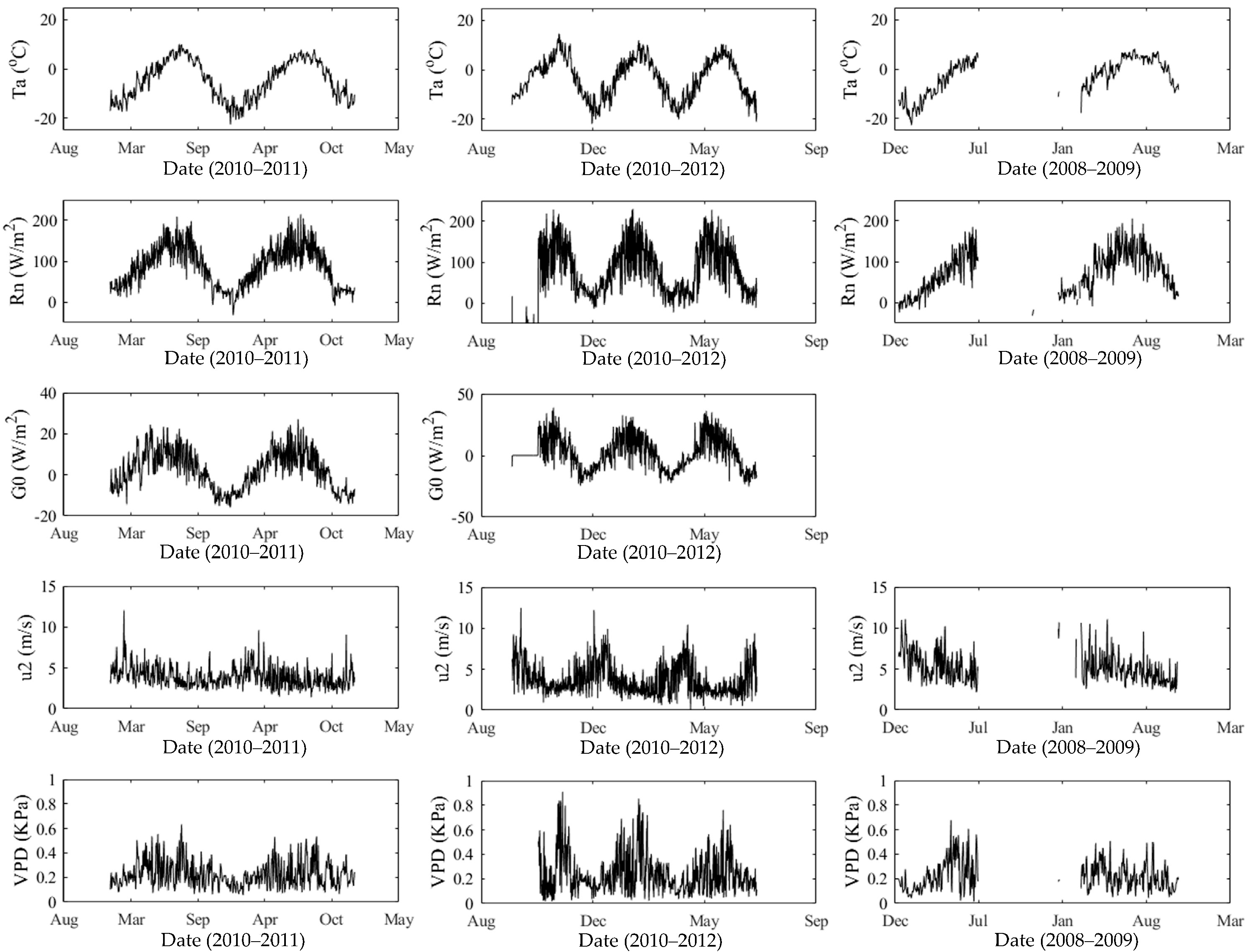
The changes in the daily available meteorological observation data at the three sites were converted and are shown in Figure 2. The patterns of Ta, Rn, G0, and VPD were similar, where the peak occurred in the summer and the minimum value in the winter. This was opposite to u2, for which the high values were in the winter and reached around 8 m/s or higher. However, the mean daily Ta was low and equal to −4.36 °C, −3.44 °C, and −3.01 °C at the three sites, respectively. It could reach −20 °C in winter. The mean daily Ta, Rn, G0, u2, and VPD in TGL, XDT, and WDL are shown in Table 2. Comparing the meteorological data from these sites, it was found that the fluctuations in the daily values of Rn, G0, u2, and VPD were greater than those of Ta. The change in ETa was more vulnerable to other factors than in Ta.

3.2. Performance of the Complementary Relationship (CR)

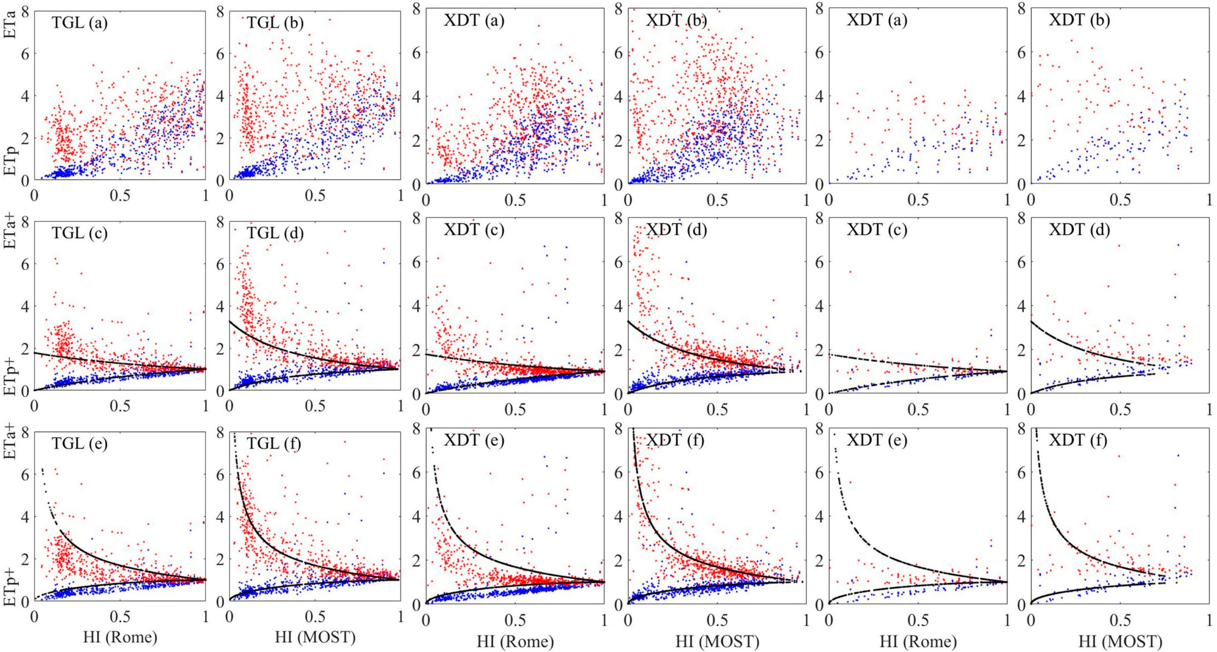
The CR was checked on a daily scale at the three sites, and the relationship between the observed ETa and the calculated ETp is shown in Figure 3. Without considering the limits of water and energy, ETa should be equal to ETp. In fact, as the supply of water decreased, ETa decreased and ETp increased in this work. The higher the value of the humidity index (HI = ETa/ETp), the more concentrated the scattered points. Comparing Figure 3a,b, the values of ETp calculated using the MOST were more discrete and greater than those using the Rome wind function. This suggests that ETp is greater in arid conditions and is consistent with the definition of potential evapotranspiration on the QTP.
In order to accurately reflect the relationship between ETa and ETp, the dimensionless term of the observed ETa and calculated ETp are also displayed, which are denoted for ETa+ (= ETa/ETw) and ETp+ (= ETp/ETw) by blue and red points in Figure 3, respectively. It was found that the difference between ETa+ and ETp+ decreased with the increase in the HI. The distribution of these scattered points corresponded well with the shape of the CR theory. These results confirm the existence of a complementary relationship at the study sites.
The simulated ETa values were also dimensionless, marked as the black points in Figure 3. The ETa+ simulated by the two methods with Rome and the MOST are shown in Figure 3c,d and Figure 3e,f, respectively. Comparing the relationship between the ETa+ and ETp+ with Rome at three sites, it was found that the ETp+ by Bouchet_1963 method (Equation (1)) was underestimated in arid conditions (HI < 0.2), as shown in Figure 3c, but both the ETa+ and ETp+ were overestimated by Brutsaert_2015 method (Equation (4)) in arid and humid conditions, as shown in Figure 3e. By contrast, both of the methods were improved by introducing the MOST, where ETa+ and ETp+ would better fit the shape of the CR theory, as shown in Figure 3d,f. In particular, the ETa+ and ETp+ by Brutsaert_2015 method with the MOST performed the best, as shown in Figure 3f, and could better improve the CR theory.

3.3. Validation of the Complementary Relationship (CR)

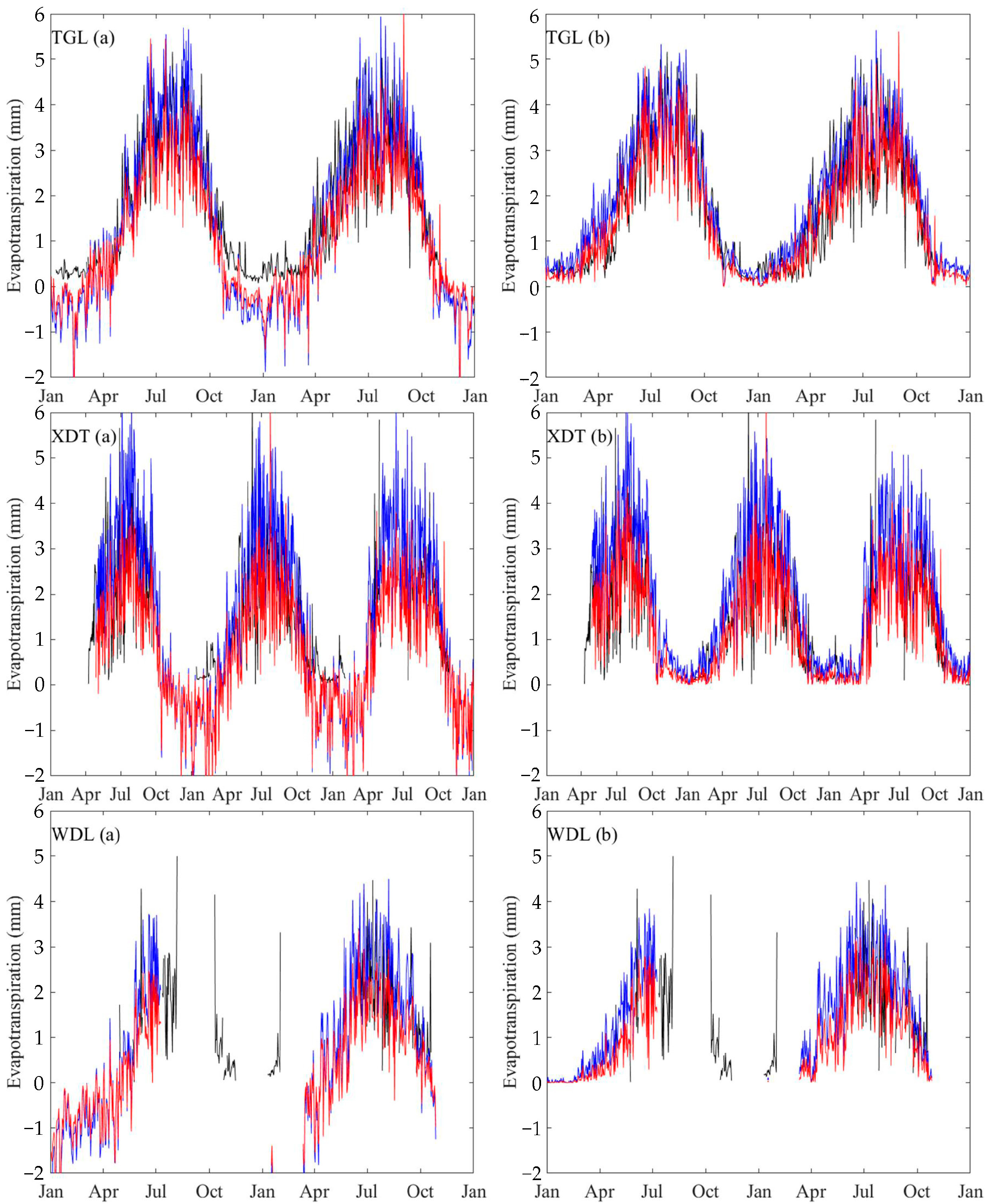
Figure 4 shows the daily simulated ETa using two different methods at the three sites. It was found that both of the changing trends of the simulated ETa were similar to the observed ETa. The peak of the daily ETa occurred in July, whereas the minimum value occurred in January and was close to 0 due to the frozen soil moisture on the land surface without an adequate supply of water. The amplitude of the ETa simulated with Bouchet_1963 method (ETa1) was lower in the cold season from October to April and higher in the warm season from May to September compared to the other observation data. In contrast, the ETa simulated with Brutsaert_2015 method (ETa2) improved significantly, especially in the cold seasons.
The simulation results are also shown by the scatter plots in Figure 5. It was obvious that the simulations with Brutsaert_2015 method (ETa2-Rome and ETa2-MOST) were much better than with Bouchet_1963 method (ETa1-Rome and ETa1-MOST). The simulation results with Brutsaert_2015 method were more concentrated around the 1:1 line. Meanwhile, it was clear that the results were affected by the wind functions. The simulations of ETa1-Rome and ETa2-Rome were significantly higher than the observed ETa. Thus, it was indicated that the MOST function is more suitable in the CR to calculate ETa on the QTP.
In this paper, the value of ε was decided by minimizing the RMSE of the observed ETa and estimated ETa. Thus, the values of ε were 0.77 and 2.27 for Equation (1) with the Rome function (Figure 3c) and the MOST function (Figure 3d) on the QTP, respectively. The Priestley–Taylor equation’s parameter α in Equation (6) was tested and verified, and the best value of α was determined for the individual method to obtain the accurate ETa. The Root Mean Square Errors (RMSEs) and correlation coefficients (r) were used to evaluate the simulation results, as shown in Table 3, with the correlation coefficients (r) tested at the 0.05 confidence level. The RMSE of ETa2 was lower than that of ETa1, although the correlation coefficients between them were not significantly different. It was clear that the minimum RMSE and the maximum correlation coefficients were obtained using Brutsaert_2015 method with the MOST function (ETa2-MOST). Thus, it could be inferred that Brutsaert_2015 method with the MOST function was appropriate for estimating ETa on the QTP by comparing these simulations.

3.4. Sensitivity of the Meteorological Factors to ETa

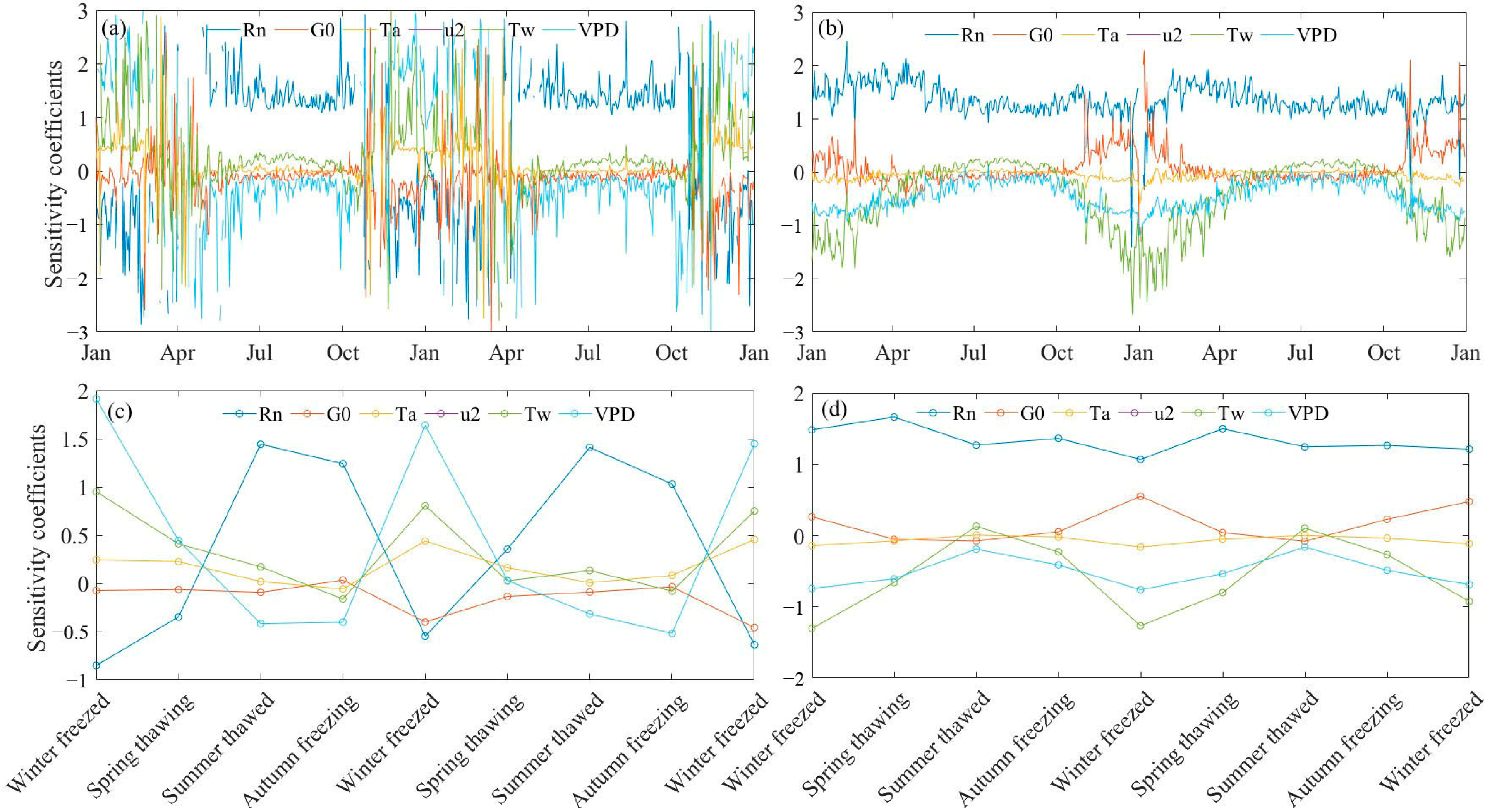
In this work, the sensitivity and contribution of ETa through Bouchet_1963 method with the MOST function and Brutsaert_2015 method with the MOST function were compared in TGL in a complete soil freeze–thaw cycle. When Bouchet’s (1963) method with the MOST function was used on the QTP, the daily average sensitivity coefficients of Rn, G0, Ta, u2, Tw, and VPD were 0.62, −0.15, 0.15, 0.14, 0.27, and 0.14, respectively. When Brutsaert_2015 method with the MOST function was used on the QTP, the daily average sensitivity coefficients of Rn, G0, Ta, u2, Tw, and VPD were 1.35, 0.08, −0.05, −0.44, −0.45, and 0.44, respectively. The positive sensitivity coefficients indicate that ETa increased with the increase in the factors and vice versa. The sensitivities of ETa on the factors using the two methods were Rn > Tw > u2 = VPD > Ta > G0 and Rn > Tw > u2 = VPD > G0 > Ta, respectively. Considering the assumed Tw in the wet environment calculated by the observed Ta, the two relationships among the factors could be expressed as Rn > Ta > u2 = VPD > G0. The sensitivities of ETa on the meteorological factors were similar for the two methods.
However, the amplitudes of vibration of the sensitivity coefficients for the two methods were different (Figure 6a,b). The change in amplitude was dramatic, as shown in Figure 6a, and are related to the uncertainties of Bouchet_1963 method. It was more sensitive to the fluctuation in the factors compared to Brutsaert_2015 method. In addition, the average sensitivity coefficients in different soil freeze–thaw periods are shown in Figure 6c,d. The change in sensitivity for ETa was more obvious in the complete soil freeze–thaw cycle for both methods.
With Bouchet_1963 method, the sensitivity coefficient of ETa on Rn peaked in the summer soil-thawed period, which played a positive role on ETa, while the opposite was found in the winter soil-frozen period (Figure 6c). The response of ETa to u2 and VPD cannot be ignored. The sensitivity coefficient of u2 and VPD peaked in the winter-frozen soil period and varied in the range of −0.52 to 1.91. The effect of u2 and VPD on ETa was very obvious in the winter soil-frozen periods and much weaker in other periods. The sensitivity coefficient of G0, Ta, and Tw showed lower variations in the complete soil freeze–thaw cycle with a relatively weak impact on ETa. The change in sensitivity coefficient of ETa on G0 was similar to that of Rn, and the coefficients of Ta and Tw were similar to those of u2 and VPD. By contrast, with Brutsaert_2015 method, Rn always had a greater positive effect on ETa without significant changes in other factors for the complete soil freeze–thaw cycle (Figure 6d). It was more obvious for the negative impact of the other factors except for G0 on ETa in the winter soil-frozen period. The impact diminished in the spring soil-thawing period and almost disappeared in the autumn soil-freezing period.
In short, the factors’ performances were different with the two methods. The sensitivity coefficient of ETa on Rn expressed the more obvious periodic changes with Bouchet_1963 method compared to with Brutsaert_2015 method. The impacts of other factors on ETa for the two methods were opposite in the freeze–thaw cycle.

3.5. Contribution of Meteorological Factors to ETa

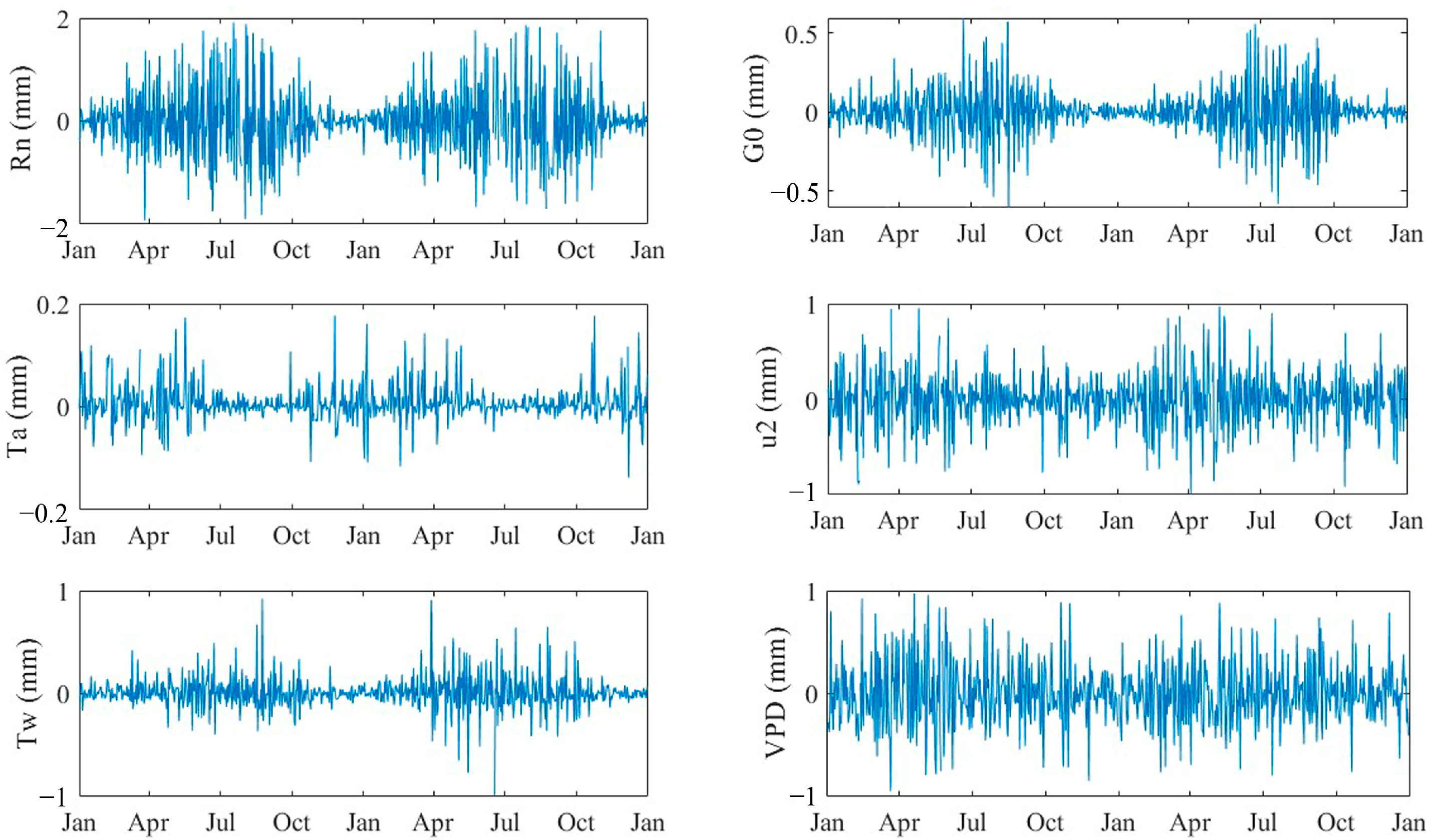
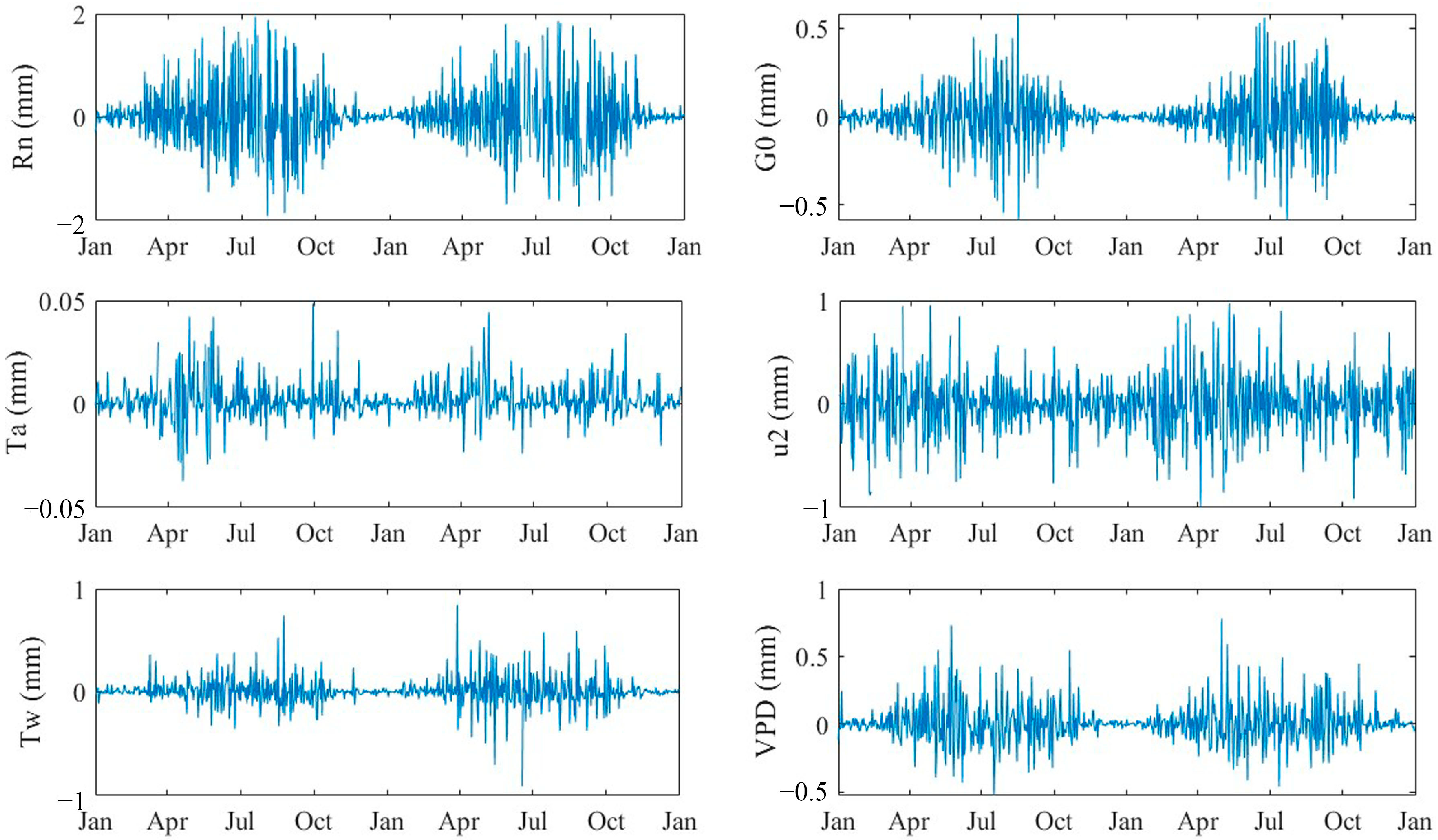
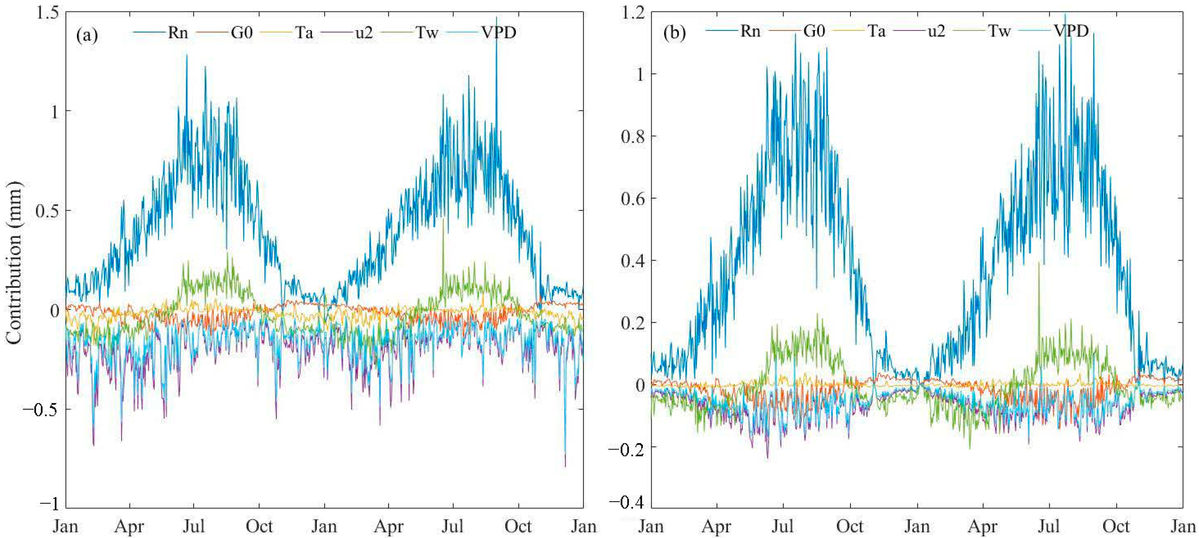
The daily contribution of Rn, G0, Ta, u2, Tw, and VPD to ETa with the two methods are compared in Figure 7 and Figure 8. The mean daily contribution rates of individual factors with Bouchet_1963 method were 54.6%, −6.3%, −1.8%, 28.7%, 7.5%, and 24.1%, respectively. As for Brutsaert_2015 method, the rates were 83.9%, −6.6%, −0.1%, 5.1%, 8.7%, and 2.6%, respectively. With Bouchet_1963 method, the contribution rates were Rn > u2 > VPD > Tw > G0 > Ta. With Brutsaert_2015 method, the contribution rates were Rn > Tw > G0 > u2 > VPD > Ta. Both Rn contributions were the largest and varied greatly, with most of the values in the range of −2 mm to 2 mm. The contributions of u2 and VPD fluctuated near ± 0.5 mm, and the contribution of Tw and G0 fluctuated slightly near ± 0.2 mm. Nonetheless, the contribution of Ta had no significant fluctuation, with values of ±0.05 mm and ±0.01 mm, respectively.
Figure 9 shows the change in accumulation values for the contribution of Rn, G0, Ta, u2, Tw, and VPD using two distinct methods. It was found that the sum of the change in ETa was about 8.98 mm and 25.00 mm using the two methods. The estimation of ETa by Brutsaert_2015 method was larger than that by Bouchet_1963method. The contribution of Rn played a different role in the two methods, which had a positive effect on ETa in the summer soil-thawed period and a negative effect in the winter soil-frozen period with Bouchet_1963 method, while always showing a positive effect with Brutsaert_2015method. In addition, the contribution of G0, Ta, Tw, and VPD also had a positive effect in the thaw-freeze period, while u2 had the opposite effect with Bouchet_1963 method. The contribution of the factors, except for G0, had a positive effect on ETa in the thaw-freeze period with Brutsaert_2015 method. Both of the maximum changes in ETa occurred in the summer soil-thawed period, and the change in ETa declined steeply in the autumn soil-freezing period, with a slight increase in the winter soil-frozen period with Brutsaert_2015 method and slight decline in the winter soil-frozen period with Bouchet_1963 method.
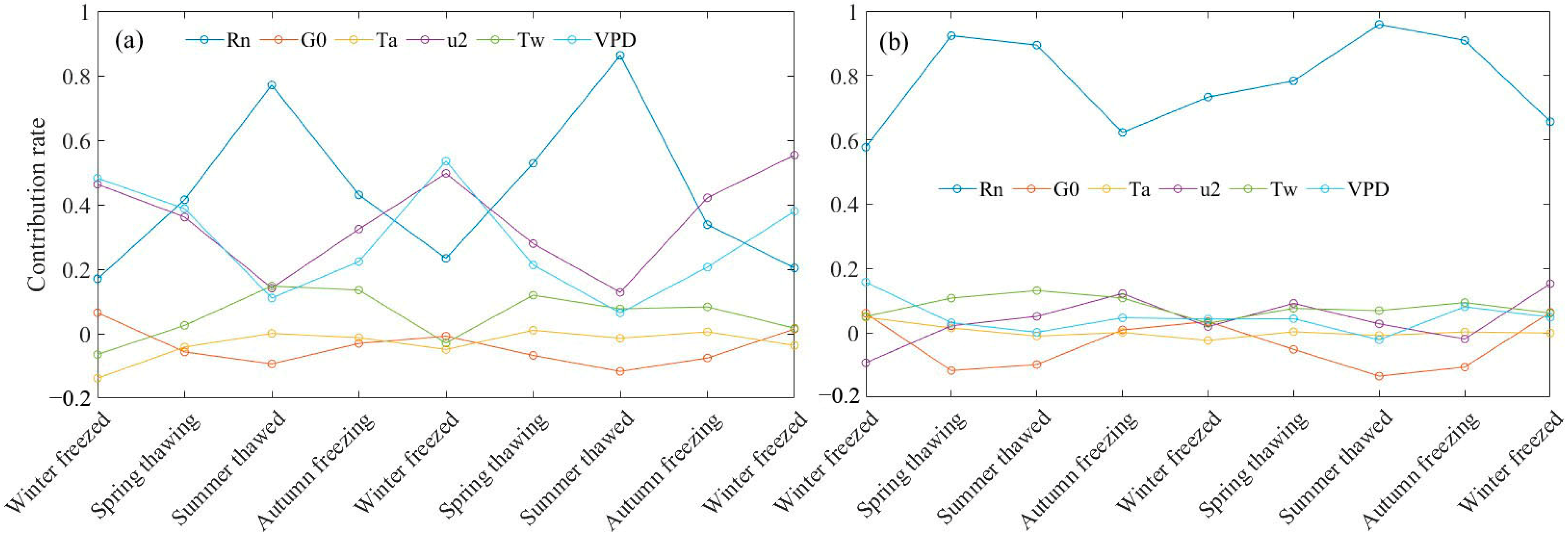
The mean contribution rates in different thaw-freeze periods are shown in Figure 10. It is clear that there were periodic changes in the contribution rate of the factors with Bouchet_1963 method. The contribution rates of Rn reached the maximum value in the summer soil-thawed period and gradually decreased in the autumn soil-freezing and winter soil-frozen periods. The changing trend of the contributions of Ta and Tw was the same with it, but the G0, u2, and VPD were opposed to it. By contrast, the contributions had no obvious periodic characteristics with Brutsaert_2015 method on a daily scale. During the thawing of the soil, the contribution of Rn, u2, and Tw increased, while VPD decreased, and Ta showed no noticeable change.

4. Discussion

The results show that the Brutsaert (2015) method, combined with the MOST, produced more reliable estimates of ETa on the QTP. This aligns with findings by Ma et al. [15], which highlighted the improved performance of CR models under complex climatic regimes. The superiority of Brutsaert_2015 method in cold and arid regions is also supported by Szilagyi and Jozsa [46], which emphasized the relevance of atmospheric feedback under low-humidity conditions.
In contrast, Bouchet_1963 linear formulation was found to consistently underestimate ETa during frozen periods and overestimate it during thawed periods. This seasonal mismatch has also been observed in other permafrost-dominated landscapes [16,48], where the fixed proportional coefficient ε in Bouchet_1963 method lacks sensitivity to changing surface and atmospheric conditions. Moreover, the analysis in this work provides a quantitative confirmation of these discrepancies, with RMSEs of 0.85–1.10 mm/day in frozen periods under Bouchet’s model.
Importantly, this study extends earlier work by comparing two wind functions (Rome and MOST) and showing their relative impact on ETp estimation. The Rome function, developed for humid environments, failed to represent wind-driven vapor transfer under high-elevation, low-pressure settings of the QTP, leading to underestimation of ETp and subsequent ETa bias. Similar limitations were noted in Ma et al.’s work [49], where ETa estimates based on the Rome function showed increasing divergence in dry seasons. According to the observations, the mean daily wind on the QTP was higher than 3.7 m/s, but the f(u) of the Rome function was underestimated when the wind speed was higher than 3.7 m/s [49]. The use of the MOST offered better adaptability to local micrometeorological conditions, enhancing CR performance, especially in frozen periods. These findings are consistent with results from Chen et al. [14], who found that MOST-based aerodynamic resistance improved land surface heat flux estimation across Tibetan alpine ecosystems.
However, the study has several limitations. First, the coefficient ε in Bouchet’s method was assumed to be constant, which may not reflect its temporal variability. Second, spatial heterogeneity in vegetation and soil properties was not fully considered.
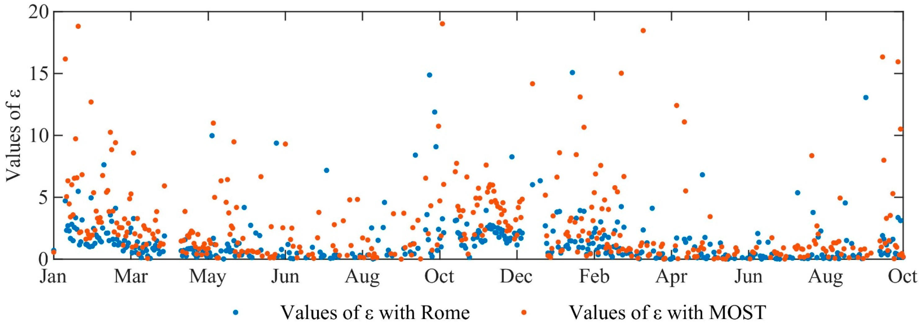
Based on the observed ETa, the daily ε could be calculated. Figure 11 shows the change in the daily ε in TGL, where it was found that the value of ε was different throughout the year. It was in the range of 1 to 10 in the cold season and 0 to 1 in the warm season. Due to a lack of observation on the QTP, it was difficult to decide what the value of ε in the climate and land surface condition is. In this paper, it was a constant that can minimize the RMSE without considering the difference of ε. Ma et al. [16] also optimized the value of ε in the Shanghu alpine steppe, which was less than 1 in the growing season in the Tibet Plateau. Therefore, the ETa was underestimated by Bouchet_1963 method in spring and winter. By contrast, the ETa simulated by Brutsaert_2015 method was close to the observed ETa without considering the coefficient ε.
In future research, incorporating remote sensing-based surface parameters and dynamic ε calibration could enhance model adaptability and accuracy. Additionally, long-term datasets are needed to assess interannual variations and climate sensitivity of CR-based ETa models in cold regions.
The amplitude of the contribution of meteorological factors to ETa fluctuated strongly on a daily scale, as shown in Figure 7 and Figure 8. By comparing the differences of two consecutive days as the variable amplitude in this work, a certain percentage (20%) of factors was usually regarded as a factor of change [48]. Based on the base value percentage amplitude method, the contributions of the meteorological factors to ETa showed a relatively stable change trend, responding to the meteorological factors without fluctuating significantly (Figure 12). This could reflect the impact of the meteorological factors on ETa, although it does not represent the true response to the change in the meteorological factors as this work does. The results based on the base value percentage amplitude method are consist with those based on the method of differences over two consecutive days.
In addition to its methodological contribution, this study addresses a gap in the existing literature by linking CR theory with freeze–thaw processes. Few studies have analyzed CR behavior across seasonal soil thermal dynamics. The freeze–thaw analysis in this work revealed clear seasonal transitions in factor sensitivity and contribution. It is conducive to understanding the relationship between the freeze–thaw process and evapotranspiration.
Overall, this study provides evidence that the Brutsaert + MOST combination is an effective approach to ETa estimation in permafrost regions. However, challenges remain in capturing spatial heterogeneity and in dynamically parameterizing ε in Bouchet-type models. These limitations provide an idea for integrating remote sensing and land surface modeling to upscale ETa estimates in the future.

5. Conclusions

This study confirmed the existence of a complementary relationship between ETa and ETp in the permafrost regions of the QTP. The ETp computed with the MOST was consistently higher than that derived from the Rome wind function, especially under dry and frozen conditions. Quantitatively, the Brutsaert_2015 method combined with the MOST achieved the best performance, with RMSE values of 0.67–0.70 mm/day and correlation coefficients (r) of 0.81–0.86 (p < 0.05) across three stations.
Sensitivity analysis showed that ETa was most responsive to the net radiation, with a daily sensitivity coefficient reaching up to 1.35. The contribution analysis revealed that the net radiation accounted for more than 80% of ETa variation under Brutsaert’s method. These findings suggest that Brutsaert’s CR model, free from reliance on an empirical ε parameter, is more robust in cold alpine environments.
Nonetheless, uncertainties remain in parameter assumptions (e.g., constant ε, assumed neutral stability), and the reliability of results is contingent upon the quality and temporal resolution of EC observations. Future studies should consider dynamic parameterization and larger spatiotemporal validation to improve the applicability of CR-based ETa models in cold and complex terrains.

Author Contributions

Conceptualization, Y.L.; Investigation, Y.X.; Data curation, Y.X. and Y.Z.; Writing—original draft, W.Y.; Writing—review & editing, A.K.; Funding acquisition, W.S. All authors have read and agreed to the published version of the manuscript.

Funding

The work was funded by the Central Government Guidance Fund for Local Sci-Tech Development in Qinghai Province (2025ZY032), the Natural Science Foundation of Xinjiang Uygur Autonomous Region (2022D01A365), and the National Natural Science Foundation of China (41901076).

Institutional Review Board Statement

Not applicable.

Informed Consent Statement

Not applicable.

Data Availability Statement

All data are available in public domain (https://data.tpdc.ac.cn/, accessed date: 7 January 2021).

Acknowledgments

We appreciate the technical support provided by Lin Zhao and the State Key Laboratory of Cryospheric Science.

Conflicts of Interest

The authors declare no conflict of interest.

Abbreviations

QTPQinghai–Tibetan Plateau
ETaActual Evapotranspiration
ETpPotential Evapotranspiration
CRComplementary Relationship
ECEddy Covariance
MOSTMonin–Obukhov Similarity Theory
RMSERoot Mean Square Error
RnNet Radiation
TaAir Temperature
RHRelative Humidity
u2Wind Speed
TwAir temperature in a wet environment
VPDSaturation and actual vapor pressure deficit

References

  1. Swelam, A.; Jomaa, I.; Shapland, T.; Snyder, R.; Moratiel, R. Evapotranspiration response to climate change. In Proceedings of the XXVIII International Horticultural Congress on Science and Horticulture for People (IHC2010): International Symposium on 922, Lisbon, Portugal, 22 August 2010. [Google Scholar]
  2. Abtew, W.; Melesse, A. Climate change and evapotranspiration. In Evaporation and Evapotranspiration: Measurements and Estimations; Springer: Dordrecht, The Netherlands, 2013; pp. 197–202. [Google Scholar]
  3. Zhao, L.; Cheng, G.; Li, S.; Zhao, X.; Wang, S. Thawing and freezing processes of active layer in Wudaoliang region of Tibetan Plateau. Chin. Sci. Bull. 2000, 45, 2181–2187. [Google Scholar] [CrossRef]
  4. Yang, K.; Wu, H.; Qin, J.; Lin, C.; Tang, W.; Chen, Y. Recent climate changes over the Tibetan Plateau and their impacts on energy and water cycle: A review. Glob. Planet. Change 2014, 112, 79–91. [Google Scholar] [CrossRef]
  5. Lei, Y.; Shi, J.; Xiong, C.; Ji, D. Tracking the atmospheric–terrestrial water cycle over the Tibetan Plateau based on ERA5 and grace. J. Clim. 2021, 34, 6459–6471. [Google Scholar] [CrossRef]
  6. Wang, K.; Dickinson, R.E. A review of global terrestrial evapotranspiration: Observation, modeling, climatology, and climatic variability. Rev. Geophys. 2012, 50, RG2005. [Google Scholar] [CrossRef]
  7. Li, Z.; Tang, R.; Wan, Z.; Bi, Y.; Zhou, C.; Tang, B.; Zhang, X. A review of current methodologies for regional evapotranspiration estimation from remotely sensed data. Sensors 2009, 9, 3801–3853. [Google Scholar] [CrossRef]
  8. Zhang, K.; Kimball, J.S.; Running, S.W. A review of remote sensing based actual evapotranspiration estimation. Wiley Interdiscip. Rev. Water 2016, 3, 834–853. [Google Scholar] [CrossRef]
  9. Penman, H.L. Natural Evaporation from Open Water, Bare Soil and Grass. Proc. R. Soc. Lond. 1978, 193, 120–145. [Google Scholar]
  10. Monteith, J.L. Evaporation and environment. Symposia of the society for experimental biology. Camb. Univ. Press (CUP) Camb. 1965, 19, 205–234. [Google Scholar]
  11. Mu, Q.; Heinsch, F.A.; Zhao, M.; Running, S.W. Development of a global evapotranspiration algorithm based on MODIS and global meteorology data. Remote Sens. Environ. 2007, 111, 519–536. [Google Scholar] [CrossRef]
  12. Su, Z. The Surface Energy Balance System (SEBS) for estimation of turbulent heat fluxes. Hydrol. Earth Syst. Sci. 2002, 6, 85–100. [Google Scholar] [CrossRef]
  13. Oku, Y.; Ishikawa, H.; Su, Z. Estimation of land surface heat fluxes over the Tibetan Plateau using GMS data. J. Appl. Meteorol. Climatol. 2007, 46, 183–195. [Google Scholar] [CrossRef]
  14. Chen, X.; Su, Z.; Ma, Y.; Yang, K.; Wen, J.; Zhang, Y. An improvement of roughness height parameterization of the Surface Energy Balance System (SEBS) over the Tibetan Plateau. J. Appl. Meteorol. Climatol. 2013, 52, 607–622. [Google Scholar] [CrossRef]
  15. Ma, N.; Szilagyi, J.; Zhang, Y. Calibration-free complementary relationship estimates terrestrial evapotranspiration globally. Water Resour. Res. 2021, 57, e2021WR029691. [Google Scholar] [CrossRef]
  16. Ma, W.; Ma, Y.; Ishikawa, H. Evaluation of the SEBS for upscaling the evapotranspiration based on in-situ observations over the Tibetan Plateau. Atmos. Res. 2014, 138, 91–97. [Google Scholar] [CrossRef]
  17. Peng, J.; Loew, A.; Chen, X.; Ma, Y.; Su, Z. Comparison of satellite-based evapotranspiration estimates over the Tibetan Plateau. Hydrol. Earth Syst. Sci. 2016, 20, 3167–3182. [Google Scholar] [CrossRef]
  18. Feng, J.; Zhang, K.; Chao, L.; Liu, L. An improved process-based evapotranspiration/heat fluxes remote sensing algorithm based on the Bayesian and Sobol’ uncertainty analysis framework using eddy covariance observations of Tibetan grass-lands. J. Hydrol. 2022, 613, 128384. [Google Scholar] [CrossRef]
  19. Hobbins, M.T.; Ramírez, J.A.; Brown, T.C.; Claessens, L.H. The complementary relationship in estimation of regional evapotranspiration: The complementary relationship areal evapotranspiration and advection-aridity models. Water Resour. Res. 2001, 37, 1367–1387. [Google Scholar] [CrossRef]
  20. Huntington, J.; Szilagyi, J.; Tyler, S.; Pohll, G. Evaluating the complementary relationship for estimating evapotranspiration from arid shrublands. Water Resour. Res. 2011, 47, W05533. [Google Scholar] [CrossRef]
  21. Bouchet, R.J. Evapotranspiration réelle et potentielle, signification climatique. Int. Assoc. Sci. Hydrol. Pub. 1963, 62, 134–142. [Google Scholar]
  22. Ramírez, J.A.; Hobbins, M.T.; Brown, T.C. Observational evidence of the complementary relationship in regional evaporation lends strong support for Bouchet’s hypothesis. Geophys. Res. Lett. 2005, 32, L15402. [Google Scholar] [CrossRef]
  23. Soylu, M.; Istanbulluoglu, E.; Lenters, J.; Wang, T. Quantifying the impact of groundwater depth on evapotranspiration in a semi-arid grassland region. Hydrol. Earth Syst. Sci. 2011, 15, 787–806. [Google Scholar] [CrossRef]
  24. Li, X.; Gemmer, M.; Zhai, J.; Liu, X.; Su, B.; Wang, Y. Spatio-temporal variation of actual evapotranspiration in the Haihe River Basin of the past 50 years. Quat. Int. 2013, 304, 133–141. [Google Scholar] [CrossRef]
  25. Chu, R.; Li, M.; Islam, A.R.M.T.; Fei, D.; Shen, S. Attribution analysis of actual and potential evapotranspiration changes based on the complementary relationship theory in the Huai River basin of eastern China. Int. J. Climatol. 2019, 39, 4072–4090. [Google Scholar] [CrossRef]
  26. Morton, F.I. Operational estimates of areal evapotranspiration and their significance to the science and practice of hydrology. J. Hydrol. 1983, 66, 1–76. [Google Scholar] [CrossRef]
  27. Brutsaert, W.; Stricker, H. An advection-aridity approach to estimate actual regional evapotranspiration. Water Resour. Res. 1979, 15, 443–450. [Google Scholar] [CrossRef]
  28. Granger, R.J.; Gray, D. Evaporation from natural nonsaturated surfaces. J. Hydrol. 1989, 111, 21–29. [Google Scholar] [CrossRef]
  29. Brutsaert, W. A generalized complementary principle with physical constraints for land-surface evaporation. Water Resour. Res. 2015, 51, 8087–8093. [Google Scholar] [CrossRef]
  30. Brutsaert, W.; Cheng, L.; Zhang, L. Spatial distribution of global landscape evaporation in the early twenty-first century by means of a generalized complementary approach. J. Hydrometeorol. 2020, 21, 287–298. [Google Scholar] [CrossRef]
  31. Kingston, D.G.; Todd, M.C.; Taylor, R.G.; Thompson, J.R.; Arnell, N.W. Uncertainty in the estimation of potential evapotranspiration under climate change. Geophys. Res. Lett. 2009, 36, L20403. [Google Scholar] [CrossRef]
  32. Pan, S.; Tian, H.; Dangal, S.R.; Yang, Q.; Yang, J.; Lu, C.; Ouyang, Z. Responses of global terrestrial evapotranspiration to climate change and increasing atmospheric CO2 in the 21st century. Earth’s Future 2015, 3, 15–35. [Google Scholar] [CrossRef]
  33. Teuling, A.J.; De Badts, E.A.; Jansen, F.A.; Fuchs, R.; Buitink, J.; Hoek van Dijke, A.J.; Sterling, S.M. Climate change, reforestation/afforestation, and urbanization impacts on evapotranspiration and streamflow in Europe. Hydrol. Earth Syst. Sci. 2019, 23, 3631–3652. [Google Scholar] [CrossRef]
  34. McKenney, M.S.; Rosenberg, N. Sensitivity of some potential evapotranspiration estimation methods to climate change. Agric. For. Meteorol. 1993, 64, 81–110. [Google Scholar] [CrossRef]
  35. Chattopadhyay, N.; Hulme, M. Evaporation and potential evapotranspiration in India under conditions of recent and future climate change. Agric. For. Meteorol. 1997, 87, 55–73. [Google Scholar] [CrossRef]
  36. Zhang, D.; Liu, X.; Hong, H. Assessing the effect of climate change on reference evapotranspiration in China. Stoch. Environ. Res. Risk Assess. 2013, 27, 1871–1881. [Google Scholar] [CrossRef]
  37. Talsma, C.J.; Good, S.P.; Miralles, D.G.; Fisher, J.B.; Martens, B.; Jimenez, C.; Purdy, A.J. Sensitivity of evapotranspiration components in remote sensing-based models. Remote Sens. 2018, 10, 1601. [Google Scholar] [CrossRef]
  38. Cawse-Nicholson, K.; Braverman, A.; Kang, E.L.; Li, M.; Johnson, M.; Halverson, G.; Anderson, M.; Hain, C.; Gunson, M.; Hook, S. Sensitivity and un-certainty quantification for the ECOSTRESS evapotranspiration algorithm–DisALEXI. Int. J. Appl. Earth Obs. Geoinf. 2020, 89, 102088. [Google Scholar]
  39. Schuur, E.A.; McGuire, A.D.; Schädel, C.; Grosse, G.; Harden, J.W.; Hayes, D.J.; Hugelius, G.; Koven, C.D.; Kuhry, P.; Lawrence, D.M.; et al. Climate change and the permafrost carbon feedback. Nature 2015, 520, 171–179. [Google Scholar] [CrossRef]
  40. Chen, R.; Kang, E.; Zhang, Z. Integrated study on the eco-hydrological process in cold regions of China. Adv. Earth Sci. 2013, 28, 355–364. [Google Scholar]
  41. Wu, Q.; Zhang, T. Recent permafrost warming on the Qinghai-Tibetan Plateau. J. Geophys. Res. Atmos. 2008, 113, D13108. [Google Scholar] [CrossRef]
  42. Zhao, X.; Liu, C.; Yang, N.; Li, Y. Diurnal and seasonal variations of surface energy and CO2 fluxes over a site in Western Tibetan Plateau. Atmosphere 2020, 11, 260. [Google Scholar] [CrossRef]
  43. Yang, Y.; Chen, R.; Song, Y.; Han, C.; Liu, Z.; Liu, J. Evaluation of five complementary relationship models for estimating actual evapotranspiration during soil freeze-thaw cycles. Hydrol. Res. 2021, 52, 431–449. [Google Scholar] [CrossRef]
  44. Brutsaert, W. Hydrology: An Introduction; Cambridge Univ. Press: New York, NY, USA, 2005; 605p. [Google Scholar]
  45. Brutsaert, W. Evaporation into the atmosphere: Theory, history and applications. Springer Sci. Bus. Media 2013, 299, 40–55. [Google Scholar]
  46. Szilagyi, J.; Jozsa, J. New findings about the complementary relationship-based evaporation estimation methods. J. Hydrol. 1982, 354, 171–186. [Google Scholar] [CrossRef]
  47. McCuen, R.H. A sensitivity and error analysis CF procedures used for estimating evaporation. J. Am. Water Resour. Assoc. 1974, 10, 486–497. [Google Scholar] [CrossRef]
  48. Liu, X.; Yang, W.; Zhao, H.; Wang, Y.; Wang, G. Effects of the freeze-thaw cycle on potential evapotranspiration in the permafrost regions of the Qinghai-Tibet Plateau, China. Sci. Total Environ. 2019, 687, 257–266. [Google Scholar] [CrossRef]
  49. Ma, N.; Zhang, Y.; Szilagyi, J.; Guo, Y.; Zhai, J.; Gao, H. Evaluating the complementary relationship of evapotranspiration in the alpine steppe of the Tibetan Plateau. Water Resour. Res. 2015, 51, 1069–1083. [Google Scholar] [CrossRef]
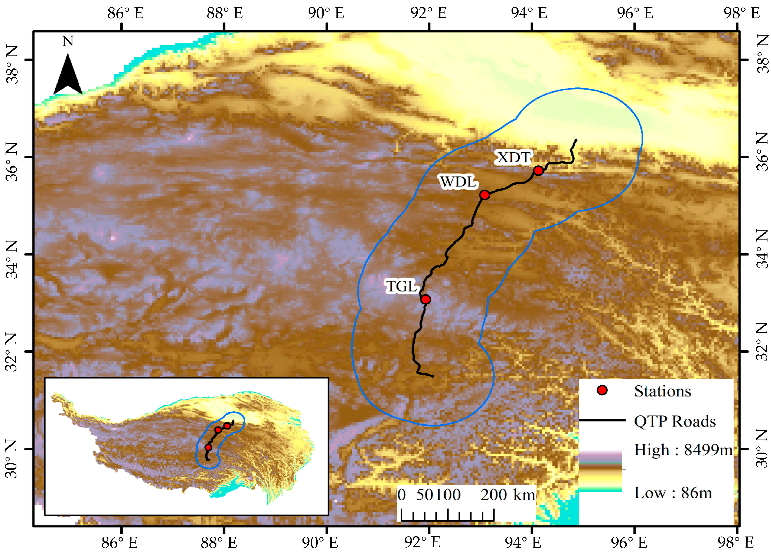
Figure 1. Elevation and distribution of three meteorological stations on the QTP.
Atmosphere 16 00932 g001
Figure 2. Daily meteorological observation (air temperature, net radiation, wind speed, vapor pressure deficit, and precipitation) of the three stations (TGL, XDT, and WDT from left to right).
Atmosphere 16 00932 g002
Figure 3. (a,b) Observed daily ETa (red points) and estimated daily ETp (blue points) plotted against the humidity index (HI) at TGL, XDT, and WDL; (c,d) normalized ETa+ and ETp+ plotted against the humidity index (HI) by Equation (1); (e,f) normalized ETa+ and ETp+ by Equation (4); the black points represent the dimensionless estimated ETa.
Atmosphere 16 00932 g003
Figure 4. CR-simulated and eddy-covariance-measured daily evapotranspiration rate from the three stations (TGL, XDT, and WDL): (a) Bouchet_1963 method; (b) Brutsaert_2015 method; the black line is the observed ETa; the blue line is the simulated ETa with Rome; the red line is the simulated ETa with the MOST.
Atmosphere 16 00932 g004
Figure 5. Scatter plots of the simulated ETa and the observed ETa;ETa-sim1-Rome and ETa-sim2 -Rome represent the results from Bouchet_1963 and Brutsaert_2015 with Rome, respectively; ETa-sim1-Rome and ETa-sim2 -Rome represent the results from Bouchet_1963 and Brutsaert_2015 with MOST, respectively.
Atmosphere 16 00932 g005
Figure 6. Sensitivity coefficients of climate factors for ETa; (a,b): diurnal sensitivity coefficient variations of climate factors; (c,d): sensitivity coefficient changes of climate factors during freeze-thaw cycles.
Atmosphere 16 00932 g006
Figure 7. The contribution of factors to ETa using Bouchet_1963 method with the MOST function.
Atmosphere 16 00932 g007
Figure 8. The contribution rate of factors to ETa using Brutsaert_2015 method with the MOST function.
Atmosphere 16 00932 g008
Figure 9. Accumulation curve of the contribution of Rn, G0, Ta, u2, Tw, and VPD (a) with Brutsaert_2015 method with the MOST function, and (b) with Bouchet_1963 method with the MOST function.
Atmosphere 16 00932 g009
Figure 10. The contribution rate of factors to ETa in different soil freeze–thaw periods (a) with Brutsaert_2015 method with the MOST function, and (b) and Bouchet_1963 method with the MOST function.
Atmosphere 16 00932 g010
Figure 11. The change in values of ε in TGL with Bouchet_1963 method with Rome and the MOST.
Atmosphere 16 00932 g011
Figure 12. The impact of the meteorological factors on ETa: (a) the contribution of the meteorological factors on ETa by Bouchet_1963 method; (b) the contribution of the meteorological factors on ETa by Brutsaert_2015 method.
Atmosphere 16 00932 g012
Table 1. List of the observed sites along the QTP engineering corridor.
Sites
(Abbr.)
Longitude (E)
Latitude (N)
Elevation
(m asl)
TopographySoil TypeGrass TypesObserved Items Time
TGL91.93°5100 High-altitude mountain, gentle slopesPermafrost soilsMeadow steppeu2, HR, Ta, Pres, P, R, heat flux, soil temperature, and moisture2010–2011
33.07°
XDT94.13°4538 Gently sloped or flatAlpine meadow soils, cryosolsAlpine meadow2010–2012
35.72°
WDL93.08°4783 Plateau basin, flat terrain Cryosols, gravelly soilsAlpine desert steppe2008–2009
35.22°
Note: TGL is Tanggula; XDT is Xidatang; WDL is Wudaoliang. u2 is wind speed; HR is relative humidity; Ta is air temperature; Pres is air pressure; P is precipitation; R is solar radiation.
Table 2. The mean daily values of the meteorological factors.
Study SitesTa (°C)Rn (W/m2)G0 (W/m2)u2 (m/s)VPD (kPa)
TGL−4.3685.572.193.940.23
XDT−3.4461.211.693.760.24
WDL−3.0171.515.190.22
Note: TGL, XDT, and WDL are Tanggula, Xidatang, and Wudaoliang, respectively. Ta is air temperature; Rn is the net solar radiation; G0 is the soil heat flux; u2 is wind speed; VPD is the actual vapor pressure deficit.
Table 3. The Root Mean Square Errors (RMSEs) and correlation coefficients (r) of ETa and calculated ETa.
SitsCounts of Available DataETaRMSEr
TGL643ETa1_Rome0.97 0.86
ETa2_Rome0.80 0.85
ETa1_MOST0.87 0.85
ETa2_MOST0.70 0.86
XDT621ETa1_Rome1.17 0.79
ETa2_Rome1.03 0.85
ETa1_MOST0.98 0.74
ETa2_MOST0.67 0.81
WDL183ETa1_Rome0.80 0.62
ETa2_Rome0.73 0.58
ETa1_MOST0.75 0.63
ETa2_MOST0.62 0.62
Disclaimer/Publisher’s Note: The statements, opinions and data contained in all publications are solely those of the individual author(s) and contributor(s) and not of MDPI and/or the editor(s). MDPI and/or the editor(s) disclaim responsibility for any injury to people or property resulting from any ideas, methods, instructions or products referred to in the content.