Article

Can a Global Climate Model Reproduce a Tornado Outbreak Atmospheric Pattern? Methodology and a Case Study

1
South Central Climate Adaptation Science Center, Norman, OK 73019, USA
2
Department of Geography and Environmental Sustainability, The University of Oklahoma, Norman, OK 73019, USA
3
Department of Earth, Atmospheric, and Planetary Sciences, Massachusetts Institute of Technology, Cambridge, MA 02139, USA
4
School of Meteorology, The University of Oklahoma, Norman, OK 73072, USA
*
Author to whom correspondence should be addressed.
Atmosphere 2025, 16(8), 923; https://doi.org/10.3390/atmos16080923
Submission received: 29 June 2025 / Revised: 27 July 2025 / Accepted: 29 July 2025 / Published: 30 July 2025
(This article belongs to the Section Meteorology)

Abstract

Tornado outbreaks can cause substantial damage, injuries, and fatalities, highlighting the need to understand their characteristics for assessing present and future risks. However, global climate models (GCMs) lack the resolution to explicitly simulate tornado outbreaks. As an alternative, researchers examine large-scale atmospheric ingredients that approximate tornado-conducive environments. Building on this approach, we tested whether patterns of covariability between WMAXSHEAR and 500-hPa geopotential height anomalies, previously identified in ERA5 reanalysis, could approximate major U.S. May tornado outbreaks in a GCM. We developed a proxy-based methodology by systematically testing pairs of thresholds for both variables to identify the combination that best reproduced the leading pattern selected for analysis. These thresholds were then applied to simulations from the high-resolution MPI-ESM1.2-HR model to assess its ability to reproduce the original pattern. Results show that the model closely mirrored the observed tornado outbreak pattern, as indicated by a low normalized root mean square error, high spatial correlation, and similar distributions. This study demonstrates a replicable approach for approximating tornado outbreak patterns, applied here to the leading pattern, within a GCM, providing a foundation for future research on how such environments might evolve in a warming climate.

1. Introduction

Tornado outbreaks, characterized by multiple tornadoes occurring in close succession, pose substantial risks to human life and property. Unlike hurricanes or floods, which develop gradually over several days and often affect vast areas, tornado outbreaks typically unfold rapidly and concentrate impacts over relatively smaller regions. Their heightened hazard potential stems from the possibility of multiple long-track tornadoes striking numerous communities [1,2]. For example, the devastating tornado outbreak of 25–28 April 2011, produced 343 tornadoes, resulted in 321 fatalities, and caused over USD 10 billion in damages [3,4,5]. Given their potentially severe consequences, advancing knowledge of tornado outbreaks is not only crucial for assessing present-day risks but also for understanding their potential future changes.
However, uncertainties remain about how a warming climate may influence the frequency and intensity of tornadic storms. Much of this uncertainty stems from two factors: (1) The small-scale and short-lived nature of tornado-producing thunderstorms, which cannot be adequately resolved by global or regional climate models [6,7], and (2) well-documented deficiencies in the tornado reporting database, which complicate the historical assessment of changes in tornado activity over time [2,8]. One way to navigate these challenges is by analyzing atmospheric ingredients, quantifications of moisture, instability, lift, and wind shear, that reflect meso- or synoptic-scale conditions conducive to tornado and tornado outbreak development. Such an ingredient-based approach leverages larger-scale variables, making it possible to assess relevant conditions in both reanalysis and model datasets. For example, a strong trough–ridge pattern in 500-hPa geopotential height, with a deep trough over the central U.S. and a downstream ridge over the eastern U.S., has been associated with conditions favorable for tornado outbreaks [9,10,11,12,13,14]. Similarly, environments with elevated values of convective available potential energy (CAPE; [15]) and sufficient vertical wind shear support the formation and sustenance of long-lived supercells capable of producing tornadoes [16,17,18,19,20].
The ingredient-based approach also serves as a valuable tool for evaluating whether global climate models can simulate environments favorable for tornado outbreaks. Prior to the interpretation of future projections, it is essential to evaluate a model’s ability to realistically simulate the historical climate for the variables and regions of interest. This validation process typically involves quantifying the agreement between observationally based and model-simulated environments. For example, Diffenbaugh et al. [21] explored the impacts of elevated greenhouse forcing on severe thunderstorm environments in the U.S. and confirmed the ability of CMIP5 models to represent severe weather conditions reasonably well. Similarly, Gensini and Mote [22] also compared observed and model-simulated severe weather environments associated with hazardous convective weather, focusing particularly on the geographical and seasonal distribution of severe thunderstorms in future projections. Trapp et al. [23] assessed the ability of models across global, regional, and convection-permitting scales to replicate key tornado-related atmospheric conditions. Trapp and Hoogewind [7] further evaluated the skill of three CMIP5 models (MIROC5, GFDL CM3, and NCAR CCSM4) in simulating future (2090-99) large-scale environments favorable for severe thunderstorms and tornadoes, emphasizing the importance of accurately representing the climatological frequency and variability of these events. These and similar studies (e.g., [24,25,26,27,28]) emphasize the need to better understand tornado-favorable environments and evaluate the capabilities of climate models to simulate them.
A recent study by Ćwik et al. [29] advanced this line of work by applying a maximum covariance analysis (MCA) to identify three primary patterns of covariability between anomalies of 500-hPa geopotential height and WMAXSHEAR, a parameter that integrates instability (i.e., CAPE) and deep-layer shear (0–6 km) [30,31], during major tornado outbreak days in May from 1950 to 2019. The high-resolution ERA5 reanalysis data used in that work allowed for an analysis of the atmospheric conditions leading up to these events, uncovering specific patterns and characteristics associated with tornado outbreaks. These identified patterns may serve as valuable references for evaluating climate model simulations and for approximating outbreak-favorable environments in future projections. However, two key questions remain. First, how stationary are these patterns over time? Temporal shifts in covariability may influence the reliability of these reference patterns for model evaluation and affect the interpretation of future projections. Second, can a global climate model reproduce outbreak-favorable atmospheric patterns identified in reanalysis?
Motivated by these questions, this study aims to (1) evaluate the temporal stationarity of the ERA5-derived patterns and (2) assess the ability of a high-resolution CMIP6 model (sixth phase of the Coupled Model Intercomparison Project [32]), MPI-ESM1.2-HR (MPI hereafter), to reproduce these large-scale atmospheric patterns and environments associated with tornado outbreaks. As highlighted by Chavas and Li [33] and others [28,34], the MPI model has shown a strong skill in reproducing the climatology of severe convective storm environments. Among CMIP6 models, MPI performed exceptionally well in capturing both the spatial pattern and magnitude of severe weather environments over North America. While climate models inherently contain biases, particularly in simulating extreme CAPE values (often linked to near-surface moist static energy biases), MPI’s overall skill and reliability in capturing the essential dynamics of severe weather environments makes it a suitable candidate for this evaluation.
To address these goals, we developed a systematic, threshold-based methodology using WMAXSHEAR and 500-hPa geopotential height anomalies to approximate outbreak-favorable patterns in both reanalysis and model data. Specifically, we tested combinations of thresholds for these two variables within ERA5. For each threshold pair, we identified the corresponding subset of days and applied an MCA to generate a proxy-based pattern, evaluating matches by maximizing spatial correlation and minimizing normalized root mean square error (nRMSE) compared to the original pattern. The pair that resulted in the best match was then applied to the full ERA5 dataset and to the MPI historical simulations. Our results indicate that the MPI model effectively reproduces the spatial structure of the observation-based pattern, providing a foundation for future efforts to analyze how these environments may evolve in a warming climate.
Accordingly, this work provides a conceptual demonstration of the method and offers a transparent, step-by-step description of the statistical techniques employed, serving as a proof of concept that this approach can both identify coherent patterns and evaluate a climate model’s ability to reproduce them. In focusing on the MPI model, we do not claim it to be the most accurate or the sole model capable of simulating severe convective storm environments but rather aim to demonstrate the viability of the method itself. It is important to note, however, that applying this approach solely to the MPI model means the findings reflect that model’s specific biases in simulating severe environments, although assessing inter-model differences is beyond the scope of this paper. To our knowledge, no prior study has combined atmospheric pattern identification, stationarity testing, and bi-variable threshold-based case selection to evaluate how effectively a climate model captures atmospheric patterns associated with tornado outbreaks. While we applied this method specifically to tornado outbreaks, it could be adapted to investigate other extreme weather phenomena that can be defined by distinct patterns and threshold-based conditions. The following sections outline the methodology, present the results, and discuss their implications for future research.

2. Materials and Methods

In this study, we expand upon the work of Ćwik et al. [29], where MCA was used to identify three leading patterns of covariability between anomalous 500-hPa geopotential heights and WMAXSHEAR anomalies associated with major U.S. May tornado outbreaks. Both the 500-hPa geopotential height anomalies and WMAXSHEAR anomalies were calculated relative to the mean values for May at each grid point, using the 1980–2014 climatology. Here, WMAXSHEAR [30,31], defined as a product of the atmospheric buoyancy and the deep-layer vertical wind shear, is used as the environmental proxy for tornado outbreak patterns. Specifically, (Equation (1)):
W M A X S H E A R = 2     C A P E     S 06
where CAPE (Convective Available Potential Energy) quantifies the potential energy available for convection [35,36,37], and S06 represents the bulk wind difference between the surface and 6 km, serving as an indicator of deep-layer shear, which is crucial for the development of supercell thunderstorms [15]. In the following subsections, we detail the data processing steps, including the use of ERA5 reanalysis data and MPI global climate model simulations, the methods applied to test atmospheric patterns identified via MCA, and the validation of the MPI model results. We also describe the spatial and temporal detrending procedures and provide a comprehensive explanation of the statistical tests used to assess the similarity and stationarity of the identified patterns.

2.1. Tornado Outbreaks and ERA5 Reanalysis Data

Consistent with Ćwik et al. [29], this analysis includes only significant tornadoes, classified as (E)F2 or greater on the (Enhanced) Fujita scale [38,39]. The selection of significant tornadoes was driven by their substantial contribution to tornado-related fatalities and the consistency of their reporting over time [40,41]. Following Ćwik et al. [11], we applied a threshold of seven or more significant tornadoes per outbreak to define major tornado outbreaks. We subsequently applied the kernel density estimation (KDE) to group the selected tornado reports into 24 h clusters within constrained regions. This was achieved by utilizing a smoothing parameter of h = 1 and a probability density function (PDF) threshold of 0.001 [42,43]. This approach yielded a database of n = 341 major tornado outbreaks across the United States from 1950 to 2019, with a specific focus on those occurring in May. The selection of May was intentional and based on its distinction as the month with the highest frequency (n = 91) of major tornado outbreaks in the U.S. [11]. Focusing exclusively on May helps reduce the influence of seasonal fluctuations in tornado-favorable environments and aligns with the methodology developed in previous work [11,29].
To obtain the variables representing the environments associated with these tornado outbreaks, we used the ERA5 reanalysis dataset, valued for its high spatiotemporal resolution and reliable representation of environments conducive to severe local storms [44,45,46]. For each major tornado outbreak in May, we extracted the 500-hPa geopotential height field and WMAXSHEAR from ERA5 at the first available time point before or at the onset of the outbreak. The anomalies for both 500-hPa geopotential height and WMAXSHEAR were calculated at each grid point by subtracting the climatological hourly mean for May, based on the 1991–2020 reference period, from the corresponding hourly values for all data from 1950 to 2019. CAPE and S06 were derived from 137 raw hybrid-sigma model levels of temperature, specific humidity, u- and v-wind components, geopotential height, and pressure using the ‘thundeR v.1.1’ R-language rawinsonde package [47,48]. For CAPE calculations, we used a 0–500 m mixed-layer parcel.

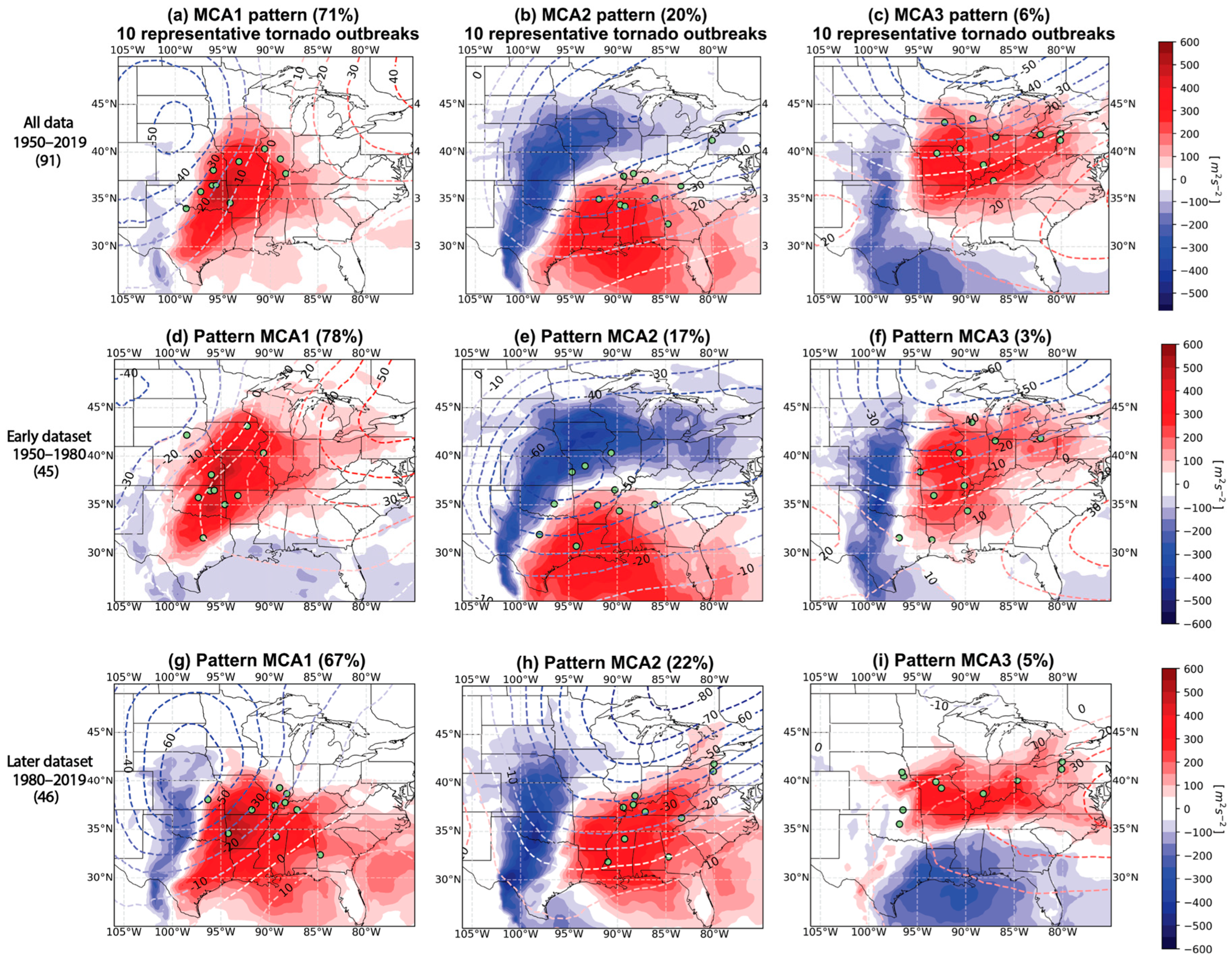
2.2. ERA5 Reanalysis: Pattern Identification and Stationarity Testing

Consistent with Ćwik et al. [29], we applied an MCA to study the multivariate relationship between WMAXSHEAR anomalies and 500-hPa geopotential height anomalies. MCA is a statistical technique that assesses the overall covariability between two sets of variables, enabling the detailed spatial identification of patterns. This method identifies patterns shared between both fields, which can provide valuable insights into the atmospheric conditions that contribute to major tornado outbreaks at both the meso- and synoptic scales. For further details on the MCA methodology, including mathematical formulas, refer to Ćwik et al. [29]. In line with the approach outlined by Ćwik et al. [29], we applied a series of steps to analyze the atmospheric patterns associated with tornado outbreaks. First, to mitigate the effects of autocorrelation in the detrending process, we filtered the dataset to include only the 1900 UTC measurements for each day in May, corresponding with the typical peak initiation time for major tornado outbreaks. We then removed long-term trends by linearly detrending the data at each grid point. After detrending, the values were weighted by the square root of the cosine of latitude to adjust for variations in grid area at different latitudes. Using this method, Ćwik et al. [29] identified three primary patterns of covariability (referred to as MCA1, MCA2, and MCA3) between anomalous 500-hPa geopotential heights and anomalous WMAXSHEAR. MCA1 is characterized by a strong WMAXSHEAR maximum centered over eastern Oklahoma, accompanied by a deep 500-hPa trough over the western U.S. and a ridge over the northeast. This pattern supports long-duration tornado outbreaks that can occur at any time of day [29]. MCA2 features a dipole in WMAXSHEAR anomalies, with negative values over the central U.S. and positive values over the mid-south, associated with a positively tilted longwave trough centered over Wisconsin. This pattern also favors prolonged tornado outbreaks. MCA3 displays positive WMAXSHEAR anomalies over Missouri and the Ohio Valley, with a 500-hPa trough over the Great Lakes, linked to shorter-lived tornado outbreaks that typically initiate in the late morning or early afternoon. In this study, we evaluate the temporal stationarity of these patterns. To do so, the original dataset of 91 tornado outbreak patterns (hereafter referred to as “all data”) was subdivided into two smaller subsets. The first subset comprised 45 tornado outbreaks that occurred from 1950 to 1980, referred to as the “early dataset.” The second subset included the remaining 46 tornado outbreaks that occurred from 1980 to 2019, referred to as the “later dataset.” MCA was performed on each subset separately, and the resulting patterns were tested using a Kolmogorov–Smirnov (KS) test and compared using normalized root mean square error (nRMSE) and spatial correlation.
To address spatial autocorrelation, which can inflate the similarity between patterns, we applied a Spatial Lag Model (SLM) to WMAXSHEAR and 500-hPa geopotential height anomalies across all MCA subset patterns. This step ensures that the residuals used in the KS, nRMSE, and spatial correlation analyses are free from significant spatial dependencies, allowing for a more precise evaluation of the spatial stationarity of the identified patterns. The SLM’s spatial weights’ matrix defines the spatial relationships among grid points in the dataset, and it includes spatial lag effects where the value at a given point is influenced by neighboring grid values. To ensure that the contribution of each grid point is proportional to the number of neighbors, the weights matrix was row standardized. The SLM is represented by (Equation (2)):
y = ρ W y + X β + ϵ
where y represents the dependent variable (e.g., WMAXSHEAR anomalies, 500-hPa geopotential height anomalies), ρ is the spatial autoregressive parameter, W is the spatial weights matrix, X is a constant term representing the intercept, β represents the regression coefficients, and ϵ represents the residuals. We tested multiple distance thresholds, ranging from 2 to 50 grid units, to determine the optimal neighborhood size that best minimized the spatial autocorrelation in the residuals. For each threshold, a Spatial Lag Model (SLM) was applied to the WMAXSHEAR and 500-hPa geopotential height anomalies, and Moran’s I was calculated to evaluate the remaining spatial autocorrelation. The threshold yielding the lowest Moran’s I was selected, and the corresponding residuals were considered spatially detrended data, ensuring minimal spatial dependencies.
With these spatially detrended residuals, we conducted KS tests, nRMSE calculations, and spatial correlation analyses to compare early and late patterns of major atmospheric conditions associated with tornado outbreaks. This analysis aimed to test the hypothesis that the atmospheric patterns are stationary over time. If the KS statistics and p-values indicate significant differences between the subsets, this would suggest temporal variability, challenging the hypothesis of stationarity. The combination of these tests provides an assessment of potential changes in the spatial structure and distribution of outbreak-supportive atmospheric patterns.

2.3. MPI Global Climate Model

2.3.1. Data Preprocessing and Comparability Testing

For the modeling component of this research, we use the MPI (MPI-ESM1.2-HR), a high-resolution coupled atmosphere–ocean Earth System Model (ESM) developed by the Max Planck Institute for Meteorology [49,50]. The atmospheric component of MPI operates with a horizontal resolution of approximately 100 km and includes 95 vertical levels, allowing for the detailed representation of atmospheric processes, including the stratosphere. This configuration aids in capturing large-scale dynamics, such as storm tracks and atmospheric blocking, which are relevant to the conditions conducive to tornado outbreaks. MPI also uses a parameterized convective scheme within ECHAM6.3 [49] to approximate smaller-scale processes within each grid cell, such as energy and moisture fluxes resulting from convective updrafts and downdrafts.
Our goal is to assess whether the historic simulation from MPI can reproduce the large-scale atmospheric pattern associated with tornado outbreaks, similar to the main pattern identified using ERA5 reanalysis data. To facilitate direct comparison, we re-gridded the ERA5 pattern from its original 0.25° × 0.25° resolution to match a coarser 0.93° × 0.93° (~103 km) of MPI using the ‘zoom’ function from the scipy.ndimage library [51]. The spatial domain remains the same as in ERA5 reanalysis, covering the region from 107° W to 75° W longitude and 24° N to 51° N latitude. The temporal range assessed spans 1980–2014 with ERA5 sampled at 6 h intervals to match the MPI output frequency. This alignment allows for a meaningful evaluation of the model’s ability to reproduce outbreak-related atmospheric covariability patterns observed in past climate conditions.
Before proceeding with the comparative analysis of patterns from ERA5 and MPI, it is crucial to ensure that the distribution of MPI and ERA5 data are similar. This alignment is essential for statistical comparability, ensuring that any observed differences do not arise from disparities between the datasets themselves. Additionally, an application for future simulations is that having similar distributions in the historical comparison increases confidence that any projected changes are due to actual climate effects rather than baseline differences between ERA5 and MPI datasets. To begin, we ensure that the MPI data are free from spatial autocorrelation, as this could misrepresent the statistical analysis. However, unlike ERA5, which focuses only on specific tornado outbreak days, the MPI data includes observations at 6 h intervals, which require adjustments for both spatial and temporal autocorrelation. To manage this process, we implemented a two-step procedure to remove spatiotemporal dependencies. First, we removed temporal autocorrelation by estimating the expected value at each time step using a first-order autoregressive model (AR(1)) applied to each grid point. The lag-1 autocorrelation coefficient ( ρ ) was estimated using the autocorrelation function (ACF), and the expected value at time t was calculated as (Equation (3)):
y ^ t = ρ y t 1  
where y ^ t is the predicted value at time t, ρ is the lag-1 autocorrelation coefficient, and y t 1 is the observed value at the previous time step. This expected value was then subtracted from the actual data to yield temporally de-autocorrelated residuals. Next, we addressed spatial autocorrelation by applying the SLM to the temporal residuals. Similarly to the approach outlined in Section 2.2 of this chapter, the removal of spatial autocorrelation was guided by testing different distance thresholds and selecting the one that produced Moran’s I values closest to zero, indicating minimal spatial autocorrelation. The resulting spatiotemporal residuals, which accounted for both temporal and spatial autocorrelation, were then used for further analysis.
To rigorously compare the adjusted residuals between the ERA5 and MPI datasets, we applied a block-based spatial permutation test along with the KS test. This approach helped address any remaining spatiotemporal dependencies and ensured that the KS test results were not affected by underlying autocorrelation. While Moran’s I is effective for measuring spatial autocorrelation within a single dataset, permutation tests are particularly useful for comparing two distinct datasets, as they account for unknown biases or sampling differences. By permuting the data, we minimize the risk that observed differences arise from random variations or inherent biases. In this case, the KS test was applied to the residuals to assess their spatial distribution, while a null distribution of KS statistics was generated through spatial permutations within 5 × 5 grid cell blocks. We performed 1000 permutations to calculate the p-value, representing the proportion of permuted KS statistics greater than or equal to the observed KS statistic. To ensure robustness, a sensitivity analysis was conducted by varying block sizes (3 × 3, 5 × 5, 7 × 7, and 10 × 10) and the number of permutations (100, 500, and 1000). For each configuration, the KS statistic and corresponding p-value were calculated, confirming that the results were not influenced by arbitrary choices of block size or permutation count.

2.3.2. Proxy-Based Pattern Detection

Finally, we describe a filtering mechanism designed to identify tornado outbreak environments using proxy variables, aiming to assess the MPI model’s ability to capture the associated atmospheric pattern. This approach relies on variables known to characterize tornado outbreaks: WMAXSHEAR anomalies (m2/s2) and 500-hPa geopotential height anomalies (m). Using ERA5 data from 1980 to 2014, we systematically tested pairs of threshold values. Specifically, threshold values for WMAXSHEAR anomalies were tested in 10 m2/s2; increments, ranging from 1500 m2/s2 to 2200 m2/s2, while thresholds for 500-hPa geopotential height anomalies were tested in 5 m intervals from −160 m to −200 m. These threshold ranges were selected to reflect the most common values found in the distribution of the two variables during historic May tornado outbreaks, while ensuring physical plausibility and model detectability. To assess the robustness of these thresholds within the historical context, we conducted a sensitivity analysis by systematically testing the full range of threshold combinations. Cases meeting each threshold pair were selected and subjected to MCA to identify the dominant atmospheric pattern linked to tornado outbreaks. For each resulting pattern, we computed the normalized RMSE (nRMSE) and spatial correlation between the ERA5 observation-based pattern and the newly generated proxy-based pattern (i.e., generated using threshold values). The threshold pair that produced a pattern with the highest correlation and lowest nRMSE was selected as the most representative of tornado outbreak environments.
Once the optimal threshold pair was determined, it was applied to the MPI historical simulations, similarly to ERA5, to identify tornado outbreak climatologies. These cases were then subjected to an MCA to derive patterns comparable to the observation-based ERA5 pattern. This approach assumes that the environmental conditions identified in ERA5 as indicative of tornado outbreaks are also applicable within the MPI data, a reasonable assumption grounded in previous studies and supported by tests confirming similar data distributions. To ensure the robustness of the selected proxy cases, we also examined their temporal distribution. This check was performed to assess whether the identified events were clustered in specific decades, which could bias the interpretation of the resulting atmospheric patterns.

3. Results

In this section, we present the results of our analysis assessing the temporal stationarity of atmospheric patterns associated with tornado outbreaks and the capability of the MPI model to reproduce these patterns.

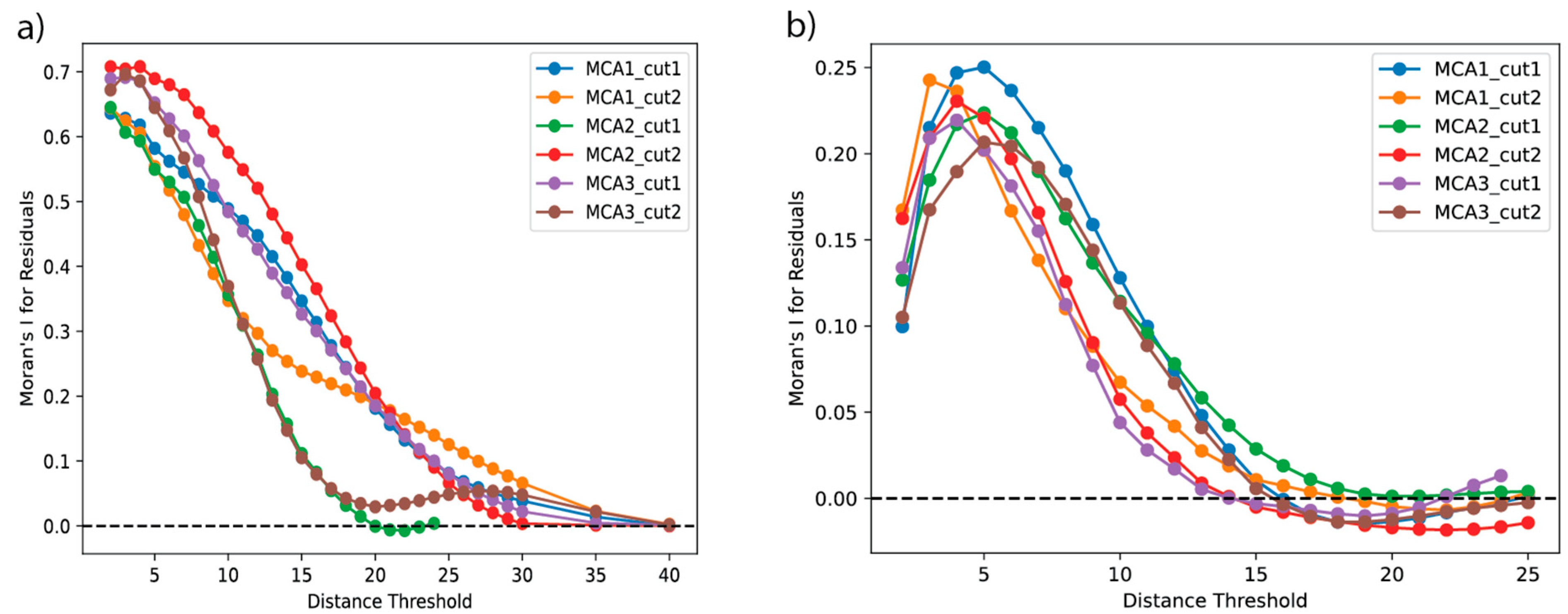
3.1. ERA5: Stationarity Testing

To investigate the temporal stationarity of tornado outbreak-associated patterns in ERA5 reanalysis, we analyzed the first three leading modes of covariability, MCA1, MCA2, and MCA3, between May 500-hPa geopotential height anomalies and anomalous WMAXSHEAR, which together account for 71%, 20%, and 6% of the covariance, respectively (Figure 1a–c). For this analysis, the data were divided into early (1950–1980) and later (1980–2019) periods, and an MCA was applied to each subset separately to assess whether these patterns remained consistent over time. The resulting modes are illustrated through homogeneous regression maps (Figure 1a–c). To highlight their geographic distribution in reference to the pattern itself, we marked ten significant tornado outbreaks per pattern, selected based on the highest values of the time series (see Figure 2b,d,f in Ćwik et al. [29]). To test if the identified spatial patterns are stationary in time, we subdivided the dataset into the early and later dataset (Section 2.2) and applied an MCA to each subset. We mapped the top three modes for the early dataset (Figure 1d–f), representing 78%, 17%, and 3% of the covariance, respectively, and the later dataset (Figure 1g–i), representing 67%, 22%, and 5%.
In general, the leading mode of covariability (MCA1) in both the early (1950–1980) and later (1980–2019) datasets exhibits slightly different spatial patterns, maxima, and minima for both variables. In the earlier dataset (Figure 1d), the WMAXSHEAR anomalies extend from central Texas northeastward through Oklahoma, Kansas, Missouri, and into the Midwest, peaking over northeastern Oklahoma and eastern Kansas with maximum values of 529 m2s−2. The negative anomalies remain restricted to parts of the western Texas panhandle and Gulf of Mexico, with local minima of −50 ton −100 m2s−2. In comparison, the later dataset (Figure 1g) shows an eastward expansion of WMAXSHEAR positive anomalies, extending from southeastern Texas to eastern Kansas and stretching from Missouri and Arkansas through Louisiana into the southeastern Atlantic states. The core of maximum WMAXSHEAR values, i.e., grid points with values above 400 m2s−2, has moved eastward and concentrated over western Arkansas, with peak values of 508 m2s−2. The western Texas panhandle continues to exhibit negative anomalies, though these become more pronounced with values reaching almost −250 m2s−2. The 500-hPa geopotential height anomalies, while generally similar in spatial positioning between the two periods, reveal a change in strength and configuration. Positive height anomalies over the eastern U.S. remain present in both periods, though they appear weaker and displaced to the southeast in the later dataset. In the earlier dataset, the core of the negative anomalies is centered over Montana and North Dakota, reaching −40 m. In the later dataset, this trough has intensified, with the core of the negative height anomalies becoming deeper (almost −70 m) and shifting southeastward over Nebraska.
The MCA2 patterns for the early and the later records (Figure 1e,h) explain 17% and 22% of covariability, respectively. In the earlier dataset, the WMAXSHEAR positive anomalies are concentrated primarily over the southern Plains, with the strongest values over western Texas and southern Kansas, reaching a maximum of 395 m2s−2. The negative WMAXSHEAR anomalies, with a minimum of −421 m2s−2 located over Iowa, extend from the Great Lakes through the U.S. central Plains. The corresponding 500-hPa geopotential height anomalies reveal an anomalously deep longwave trough centered over Kansas and Missouri, highlighting an intensified trough compared to the climatological average. In contrast, the later dataset shows an eastward expansion of positive WMAXSHEAR anomalies, covering a broader area from Texas through Arkansas, Missouri, and Mississippi, reaching the northeastern U.S. and southeast, with peak values of 385 m2s−2. The negative WMAXSHEAR anomalies deepened (minimum of −488 m2s−2) and shifted westward, reduced their presence in the Midwest and concentrated mostly over the central U.S. Great Plains. The 500-hPa geopotential height anomalies in the later period show a pronounced anomalous positive-tilt longwave of negative values, centered over eastern Ontario extending southwestward throughout entire domain.
In both the earlier and later record, MCA3 (Figure 1f,i) explains the smallest amount of covariability, i.e., 3% and 5%, respectively. In the earlier dataset, the strongest positive WMAXSHEAR anomalies, with a maximum of 346 m2s−2, were located over Missouri and Illinois, extending across the northern U.S. through Ohio to Pennsylvania. The negative WMAXSHEAR anomalies were located over the central U.S. Great Plains with a minimum of −436 m2s−2 over western Oklahoma. The 500-hPa geopotential height anomalies show a deep trough with negative anomalies centered over western Ontario, with the strongest anomalies reaching −62 m. This trough is flanked by two regions of weak positive anomalies: one over eastern New Mexico and another over the western central Atlantic. In the later dataset, maximum positive WMAXSHEAR anomalies remain strongest over Missouri and Illinois (379 m2s−2) but with similar magnitude; they also extend farther eastward into Ohio and northern Kentucky. Meanwhile, negative anomalous WMAXSHEAR disappear from the U.S. Great Plains region and occur instead over the Gulf of Mexico, with the lowest values over Louisiana (−293 m2s−2). Only a small area of weak anomalous negative 500-hPa geopotential height (−11 m) remains over southwestern Ontario and Minnesota. Meanwhile, the positive anomalies over the western central Atlantic have shifted slightly northward and become spatially more prominent.
The application of the SLM effectively reduced spatial autocorrelation across all MCA patterns for both variables, leading to less biased outcomes in subsequent statistical analyses. As shown in Figure 2, increasing the distance threshold (measured in grid points) resulted in a rapid decrease in Moran’s I values for all subsets and patterns (MCA1, MCA2, and MCA3). For the 500-hPa geopotential height anomalies, Moran’s I values approach zero (Moran’s I ~ 0) at thresholds between 20 and 35 grid points, depending on the subset and mode, suggesting that this range is optimal for minimizing spatial autocorrelation. In contrast, the decline in Moran’s I for WMAXSHEAR anomalies occurred more rapidly, reaching near-zero levels around the 15–20 grid unit range.
Our results (Table 1) indicate that none of the three patterns identified for 500-hPa geopotential height anomalies are temporally stationary, as all show significant differences between early and late periods. For WMAXSHEAR, the results are more nuanced: MCA1 and MCA2 show significant differences, while MCA3 has a p-value of 0.449, which does not meet the typical threshold for significance but also does not confirm stationarity. This suggests that MCA3 may be comparatively more stable than MCA1 and MCA2, though this should be interpreted cautiously. These findings highlight that large-scale structures associated with tornado outbreaks are not static but are evolving over time.
Given the lack of stationarity across all patterns, we intentionally focus our subsequent analysis solely on MCA1 for two primary reasons. First, MCA1 explains the largest fraction of covariability in the dataset, making it a particularly informative pattern for understanding outbreak-supportive environments, as it best characterizes the typical or dominant way in which the two fields (WMAXSHEAR and 500-hPa height anomalies) co-vary during tornado outbreaks. We restrict this analysis to the 1980–2014 period to ensure relevance to contemporary conditions and to match the temporal range of the MPI simulations. Second, MCA1 closely resembles large-scale patterns linked to tornado activity in previous studies, including the Pacific Ridge regime described by Tippett et al. [13] and similar configurations noted by Agee et al. [52], Gensini and Brooks [27], and Li et al. [45]. In ERA5, MCA1 features a deep 500-hPa trough over the western and central U.S., with ridging to the east, enhancing low-level moisture transport and instability across the central Plains. This structural similarity further supports MCA1 as the representative pattern for outbreak environments in both reanalysis and model simulations.
To further justify this focus, we examined the characteristics of 10 representative tornado outbreaks from each MCA group (MCA1, MCA2, and MCA3), the same cases shown in Figure 1. Outbreaks associated with MCA1 produced a higher mean number of tornadoes per event (13.6) compared to MCA2 (10.9) and MCA3 (9.9) and also exhibited greater numbers of strong tornadoes (EF2–EF5), with totals of 136, 109, and 99, respectively (Table 2). While MCA1 occurs more frequently in the full historical record and may therefore capture a broader range of environments, including more extreme cases, we limited this comparison to an equal number of representative outbreaks per MCA group to reduce bias and enable a more balanced assessment. These findings support MCA1 as not only a dominant synoptic pattern but also one linked to more intense outbreaks.

3.2. Pattern Comparison Between ERA5 and MPI Model

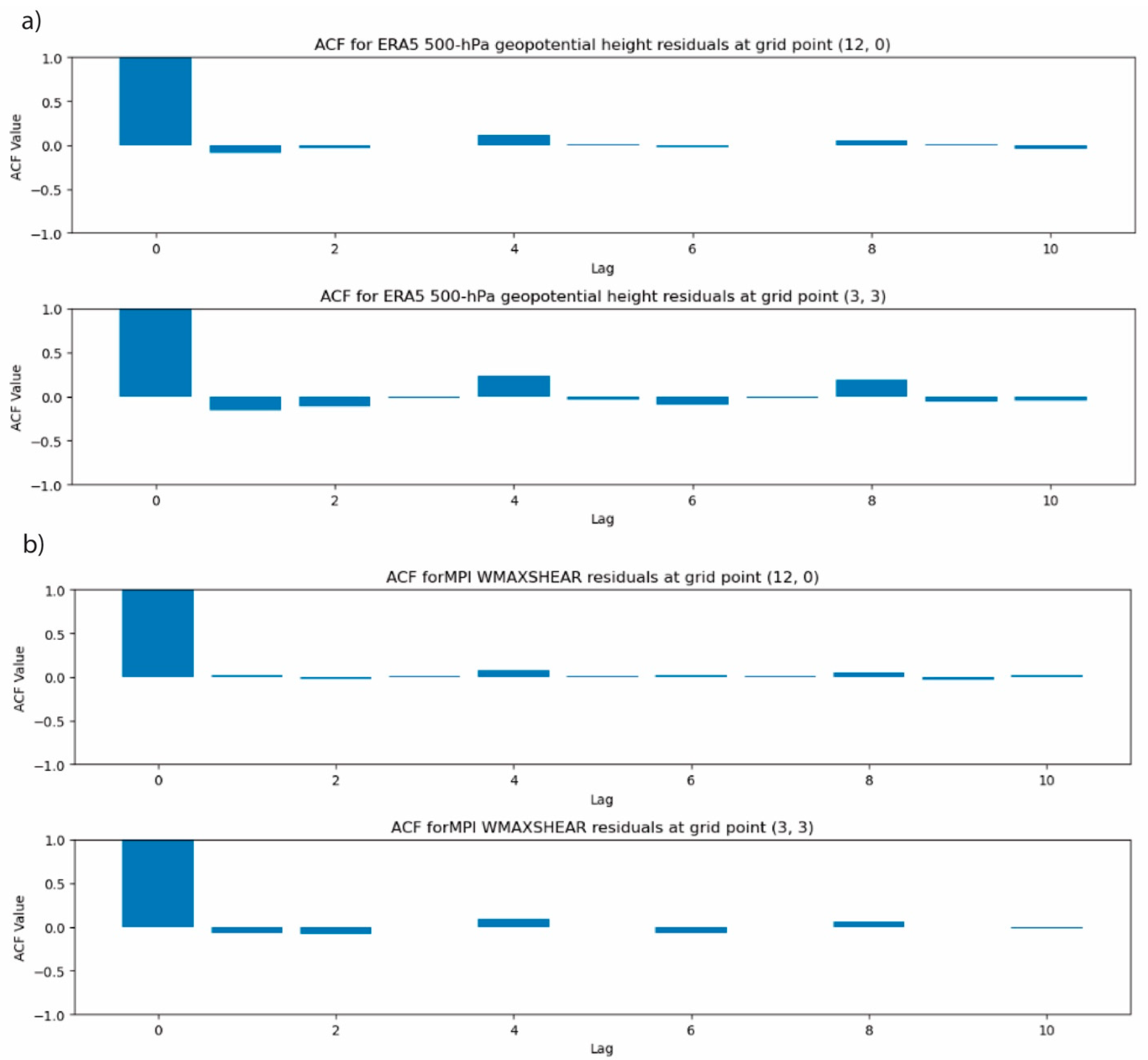
3.2.1. Data Distributions and Autocorrelation

In this subsection, we verified that ERA5 and MPI data distributions were similar to avoid introducing biases. Figure 3 shows overlapping density curves for both WMAXSHEAR and 500-hPa geopotential height anomalies, suggesting a general agreement between the two datasets. A slightly low bias is evident in the MPI data for both variables. However, before applying any statistical tests, it was necessary to address the spatial and temporal autocorrelation present in both datasets.
Temporal autocorrelation was evaluated using the autocorrelation function (ACF) for 6-hourly data (Figure 4a,b), revealing a rapid decline within the first few lags, indicating limited short-term memory in both datasets. Spatial autocorrelation was mitigated by applying a spatial weights matrix, reducing artificial similarity between neighboring grid points. Finally, we used a Kolmogorov–Smirnov (KS) test to compare the spatial distributions of the residuals, employing 1000 spatial permutations within 5 × 5 grid blocks to generate a null distribution. The results indicated no statistically significant differences between MPI and ERA5 residuals (KS statistic: 0.043, p = 0.1 for WMAXSHEAR; 0.058, p = 0.1 for 500-hPa geopotential height anomalies), and these outcomes remained consistent across different block sizes and permutation counts.

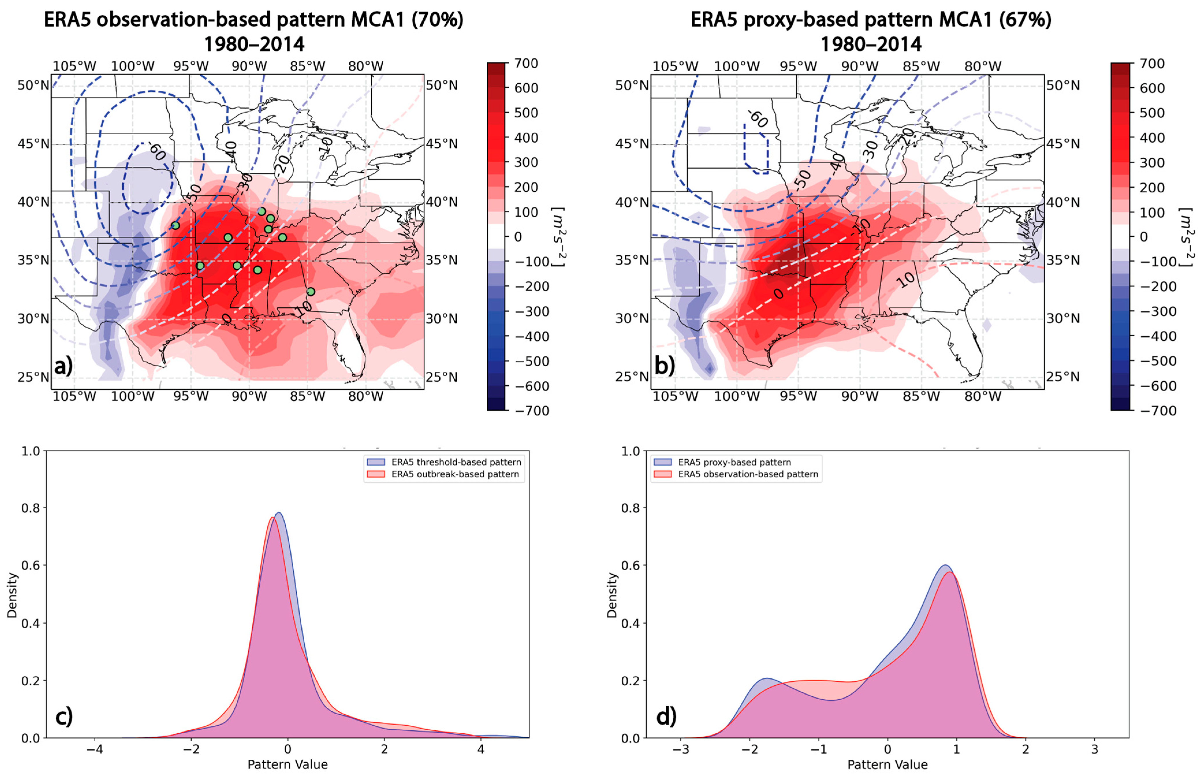
3.2.2. ERA5 Observation-Based vs. ERA5 Proxy-Based Pattern

Given a lack of significant differences between the ERA5 and MPI datasets, we proceeded to establish thresholds for identifying tornado outbreak conditions. This involved a proxy-based technique to select optimal values for WMAXSHEAR and 500-hPa geopotential height anomalies that best captured the climatological features of outbreak days. Systematic threshold testing (Section 2.3) identified an optimal pair: 1650 m2s−2 for WMAXSHEAR anomalies and −160 m for 500-hPa geopotential height anomalies. This combination produced the lowest normalized root mean square error (nRMSE) values, 0.12 for anomalous WMAXSHEAR and 0.11 for anomalous 500-hPa geopotential height, and the highest spatial correlations, at 0.71 and 0.92, respectively. When these threshold values were applied to the full ERA5 daily dataset, we identified 52 cases that met the criteria, which were subsequently analyzed using an MCA. While 45 historic major outbreaks were documented in the ERA5 period (1980–2014), the thresholding approach was not intended to recover exact dates but rather to identify environments resembling those associated with tornado outbreaks. The resulting proxy-based pattern closely mirrored the observed tornado outbreak pattern (Figure 5), indicating its reliability as a proxy for outbreak climatology.
Specifically, for WMAXSHEAR, the maximum value of positive anomalies in the observation-based pattern (Table 3, 496.8 m2s−2) was lower than the proxy-based pattern (661.4 m2s−2), suggesting that the proxy-based approach captured more extreme positive WMAXSHEAR anomalies. The mean and median in WMAXSHEAR for the observation-based pattern was higher, indicating that the observation-based dataset, on average, contained stronger values, and that the proxy-based pattern is more centered around weaker WMAXSHEAR values. The remaining metric values were similar, indicating comparable lower and upper bounds.
After removing spatial autocorrelation, we evaluated both variables using the KS test, nRMSE, and spatial correlation. For WMAXSHEAR, the KS statistic was 0.0362 (p = 0.42), with an nRMSE of 0.068 and a spatial correlation of 0.82. For 500-hPa geopotential height anomalies, the KS statistic was 0.053 (p = 0.071), with an nRMSE of 0.085 and a spatial correlation of 0.96. These results indicate a high degree of similarity between the ERA5 observation-based and ERA5 proxy-based patterns for both variables. The KS test results (p-values > 0.05) suggest no significant difference in the distributions, while the nRMSE values show a good fit between observed and simulated data, with WMAXSHEAR having a slightly better agreement. The spatial correlation values of 0.82 for WMAXSHEAR and 0.96 for geopotential height further reinforce the similarity in spatial patterns. As shown in Figure 5c,d, the distribution comparison highlights the alignment between the two patterns, supporting the validity of the filtering approach.

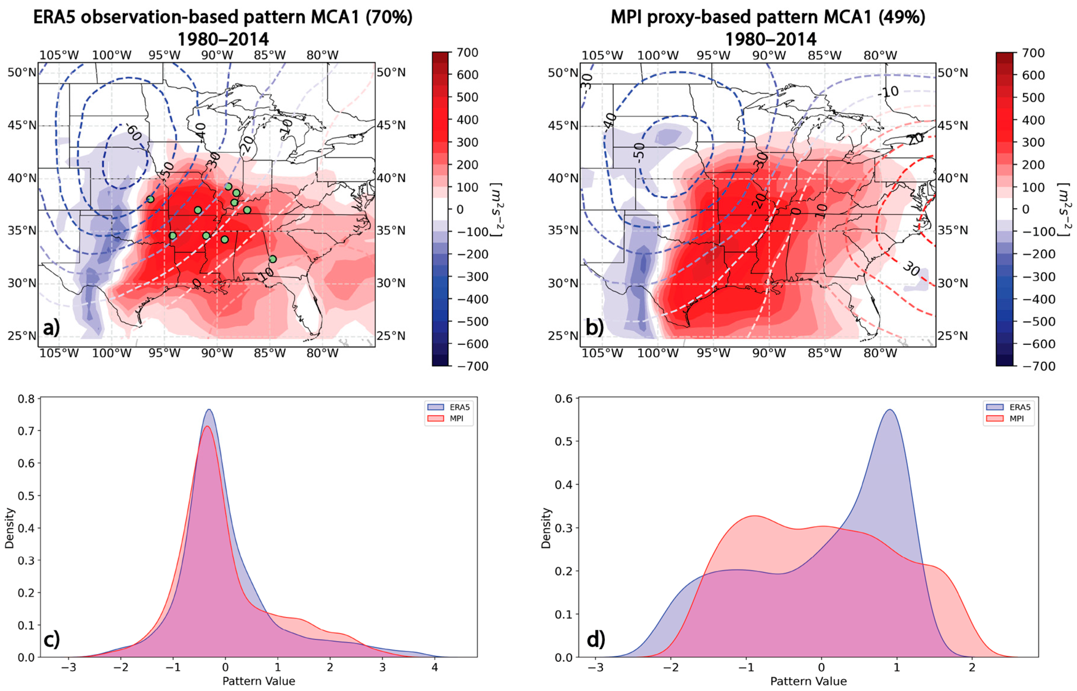
3.2.3. ERA5 Observation-Based vs. MPI Proxy-Based Pattern

Finally, we present the results of comparing the observation-based pattern from ERA5 with the proxy-based pattern identified in MPI (Figure 6). Threshold values applied to both variables in the MPI dataset resulted in the identification of 80 cases that met the criteria, which were then analyzed using MCA. The comparison of WMAXSHEAR anomalies between the two datasets yielded a KS statistic of 0.062 (p = 0.021), indicating statistically significant differences between the distributions. The nRMSE for WMAXSHEAR was 0.09, with a high spatial correlation of 0.83, indicating a strong alignment between the patterns in the two datasets. For 500-hPa geopotential height anomalies, the KS statistic was 0.15 (p = 0), suggesting a statistically significant difference between the distributions. However, the spatial correlation was notably high (0.89) and the nRMSE was relatively low (0.13), indicating that, despite differences in the distribution, the spatial pattern was well captured in the MPI compared to ERA5. Both variables exhibited similar maximum and minimum values across the datasets (see Table 4), reinforcing the similarity in the extreme values. The differences in distribution, particularly for 500-hPa geopotential height anomalies, highlight subtle discrepancies in how these patterns are represented in the MPI’s simulations.
Also, to support the assumption of temporal independence, we present the year-wise distribution of the selected proxy cases in both ERA5 (n = 52) and MPI (n = 80) (Figure 7). Ensuring temporal independence is important because if the distribution of cases were heavily concentrated in specific temporal segments (e.g., a single decade), it could lead to overlap between training and validation subsets, thereby limiting the generalizability of our findings. The selected cases span the 1980–2014 period without notable clustering in any particular decade, suggesting that the identified environments are not biased toward specific periods of the historical record.

4. Discussion

In this study, we build on the findings of Ćwik et al. [29] to address two primary research questions: (1) whether atmospheric patterns from the ERA5 reanalysis data, associated with observed major U.S. tornado outbreaks in May, are stationary over time, and (2) whether the MPI global climate model, a participant in CMIP6, can reproduce the dominant covariability pattern (MCA1) between WMAXSHEAR anomalies and 500-hPa geopotential height anomalies observed in ERA5 reanalysis data. By examining these aspects, we seek to deepen our understanding of the ability of a global climate model in simulating historical severe weather environments and synoptic patterns linked to tornado outbreaks.
Our analysis of the leading three modes of covariability (MCA1, MCA2, and MCA3) in ERA5 across early (1950–1980) and later (1980–2019) periods revealed clear spatial and intensity shifts, confirming non-stationarity. MCA1, which accounts for the largest portion of covariance (78% in the early period and 67% in the later period), showed changes in both anomaly positioning and intensity. In particular, the strongest positive WMAXSHEAR anomalies in the later period expanded southeastward, suggesting a shift in tornado outbreak-favorable conditions toward the southeastern U.S., consistent with recent studies [26,27,52]. This shift is further supported by an eastward displacement of the tornado outbreak centroids locations. New negative WMAXSHEAR anomalies emerged over the western Great Plains, hinting at weaker supportive conditions there. For 500-hPa geopotential height anomalies, we observed a southeastward intensification, signaling a stronger synoptic-scale forcing in areas farther east. The spatial non-stationarity of these atmospheric patterns, such as in MCA1, underscores changing risk profiles for severe weather over time.
A critical component of our analysis involved removing spatial autocorrelation, a step often overlooked in similar studies. By eliminating these artificial spatial dependencies before applying statistical tests, we ensured that observed similarities between reanalysis and model patterns were not artifacts of spatial proximity, thereby enhancing the credibility of our comparisons. This added layer of methodological rigor sets a precedent for future model validation studies, where ignoring spatial autocorrelation can obscure or exaggerate true differences [23,25].
To approximate tornado outbreak conditions in MPI, we applied a novel proxy-based filtering method using ERA5-derived thresholds for WMAXSHEAR and 500-hPa geopotential height anomalies. While proxy-based approaches have been explored previously (e.g., [53,54,55]), this study is the first to systematically derive and apply specific threshold combinations to a global climate model to reproduce a historically observed outbreak-favorable atmospheric pattern. By using two physically meaningful and well-represented variables, our method avoids reliance on complex indices such as STP, which are difficult to simulate accurately in GCMs [46]. Applying the selected thresholds and conducting an MCA produced a proxy-based pattern in the MPI that closely resembled the ERA5 observation-based pattern, as indicated by strong spatial correlations in both variables. Although the MPI tended to overestimate the number of outbreak-like events, this outcome is consistent with its design emphasis on representing large-scale climatological environments rather than replicating specific events [22,29]. The strong agreement between MPI and ERA5 patterns underscores the effectiveness of our proxy-based approach in capturing the large-scale atmospheric configurations associated with tornado outbreaks. To our knowledge, this is the first study to combine stationarity testing, spatial autocorrelation correction, and proxy-based pattern reconstruction using two physically meaningful variables within a GCM.
While our analysis centers on MCA1 due to its dominant explanatory power, we acknowledge that MCA2 also accounts for a meaningful portion of the covariability, particularly in the later period, where its relative contribution increases. This shift may suggest emerging complexities or a diversification of the large-scale atmospheric patterns associated with tornado outbreaks. Future work investigating whether MCA2 is similarly reproducible by climate models such as MPI, and whether its increasing role reflects evolving outbreak-supportive environments, would contribute to a more comprehensive understanding of changing risk profiles.
Although this study focuses solely on the MPI model, selected for its demonstrated skill in simulating severe convective environments, applying this threshold-based method to additional climate models would be a valuable next step. While a multi-model evaluation is beyond the scope of the present study, such an effort could help assess the broader applicability of the approach and examine how model-specific differences influence the representation of outbreak-favorable environments. We acknowledge that relying on a single model may limit the generalizability of our results, and we encourage future work to test this methodology across multiple CMIP6 models. In parallel, a companion study builds on the methodology developed in this paper to analyze scenario-based projections and investigate how outbreak-supportive environments may evolve under anthropogenic climate warming. Together, these efforts contribute to a more comprehensive understanding of model performance and the potential future behavior of tornado outbreaks. Future applications of this methodology could also explore other months and seasons, particularly the cool season, when tornado-supportive environments differ from the CAPE-dominated patterns typical of May.
Finally, the findings on the non-stationarity of atmospheric patterns associated with tornado outbreaks contribute to the broader conversation on climate adaptation and risk management by emphasizing the need to integrate evolving risk profiles into building codes, emergency response plans, and public awareness initiatives to mitigate severe weather impacts [27,56]. These findings also lay the groundwork for future research into how outbreak-supportive environments may evolve under climate change, aiming to refine adaptation strategies while addressing uncertainties in projections of severe weather.

Author Contributions

Conceptualization, P.Ć. and R.A.M.; methodology, P.Ć.; software, P.Ć.; validation, P.Ć., R.A.M., F.L. and J.C.F.; formal analysis, P.Ć.; investigation, P.Ć.; resources, P.Ć. and F.L.; data curation, P.Ć. and F.L.; writing—original draft preparation, P.Ć.; writing—review and editing, P.Ć., R.A.M., F.L. and J.C.F.; visualization, P.Ć.; supervision, R.A.M. and J.C.F.; project administration, R.A.M.; funding acquisition, R.A.M. All authors have read and agreed to the published version of the manuscript.

Funding

This research received no external funding. The APC was funded by the University of Oklahoma Libraries’ Open Access Fund.

Institutional Review Board Statement

Not applicable.

Informed Consent Statement

Not applicable.

Data Availability Statement

The U.S. tornado reports were downloaded from the Storm Prediction Center Storm Data (https://www.spc.noaa.gov/wcm/data/1950-2022_actual_tornadoes.csv, accessed on 1 February 2021). The U.S. state boundaries, used in mapping, are from the United States Census Bureau’s 2017 Cartographic Boundary Files MAF/TIGER geographic database at the county level with 20 m (1:20,000,000) resolution (available at: https://www.census.gov/geographies/mapping-files/2017/geo/kml-cartographic-boundary-files.html, accessed on 1 September 2021 or alternatively at: https://www2.census.gov/geo/tiger/GENZ2017/kml/cb_2017_us_nation_20m.zip, accessed on 1 September 2021). The ERA5 reanalysis data are provided by the European Centre for Medium-Range Weather Forecasts (ECMWF), Copernicus Climate Change Service (C3S) at Climate Data Store (CDS). For more details, refer to Hersbach et al. [57]. Raw ERA5 data was post-processed using the thundeR R language rawinsonde package available at: https://github.com/bczernecki/thundeR, accessed on 1 September 2021. We would like to acknowledge high-performance computing support from the Derecho system (https://doi.org/10.5065/qx9a-pg09, accessed on 1 September 2021) and Casper system (https://ncar.pub/casper, accessed on 10 August 2023) provided by the NSF National Center for Atmospheric Research (NCAR) sponsored by the National Science Foundation, as well as the computational resources provided by Purdue Rosen Center for Advanced Computing. We also acknowledge the open-source Python community. Six-hourly CMIP6 model historical and future experiment data were accessed from https://esgf-node.llnl.gov/search/cmip6, accessed on 1 September 2021.

Acknowledgments

This research was supported by the South Central Climate Adaptation Science Center, the Office of the Vice President for Research, and the Department of Geography and Environmental Sustainability at the University of Oklahoma. Financial support was provided by the University of Oklahoma Libraries’ Open Access Fund. ERA5 data used in this work was post-processed with a thundeR v.1.1 package. The authors would like to acknowledge high-performance computing support from Cheyenne (https://www.cisl.ucar.edu/ncar-supercomputing-history/cheyenne accessed on 1 July 2025) provided by NCAR’s Computational and Information Systems Laboratory, sponsored by the National Science Foundation, for the simulation and data analysis performed for this work. The authors also thank the four anonymous reviewers for their constructive comments, which helped improve this article.

Conflicts of Interest

The authors declare no conflicts of interest.

References

  1. Brooks, H.E. On the relationship of tornado path length and width to intensity. Weather Forecast. 2004, 19, 310–319. [Google Scholar] [CrossRef]
  2. Ćwik, P.; McPherson, R.A.; Brooks, H.E. What is a tornado outbreak? Perspectives through time. Bull. Am. Meteorol. Soc. 2021, 102, E817–E835. [Google Scholar] [CrossRef]
  3. NOAA. State of the Climate: Tornadoes, Annual 2011. National Centers for Environmental Information. 2011. Available online: https://www.ncei.noaa.gov/access/monitoring/monthly-report/tornadoes/201113 (accessed on 1 March 2025).
  4. Knupp, K.R.; Murphy, T.A.; Coleman, T.A.; Wade, R.A.; Mullins, S.A.; Schultz, C.J.; Schultz, E.V.; Carey, L.; Sherrer, A.; McCaul, E.W., Jr.; et al. Meteorological overview of the devastating 27 April 2011 tornado outbreak. Bull. Am. Meteorol. Soc. 2014, 95, 1041–1062. [Google Scholar] [CrossRef]
  5. Chasteen, M.B.; Koch, S.E. Multiscale aspects of the 26–27 April 2011 tornado outbreak. Part I: Outbreak chronology and environmental evolution. Mon. Weather Rev. 2021, 150, 309–335. [Google Scholar] [CrossRef]
  6. Trapp, R.J.; Diffenbaugh, N.S.; Brooks, H.E.; Baldwin, M.E.; Robinson, E.D.; Pal, J.S. Changes in severe thunderstorm environment frequency during the 21st century caused by anthropogenically enhanced global radiative forcing. Proc. Natl. Acad. Sci. USA 2007, 104, 19719–19723. [Google Scholar] [CrossRef]
  7. Trapp, R.J.; Hoogewind, K.A. The realization of extreme tornadic storm events under future anthropogenic climate change. J. Clim. 2016, 29, 5251–5265. [Google Scholar] [CrossRef]
  8. Tippett, M.K.; Allen, J.T.; Gensini, V.A.; Brooks, H.E. Climate and hazardous convective weather. Curr. Clim. Change Rep. 2015, 1, 60–73. [Google Scholar] [CrossRef]
  9. Mercer, A.E.; Shafer, C.M.; Doswell, C.A., III; Leslie, L.M.; Richman, M.B. Synoptic composites of tornadic and nontornadic outbreaks. Mon. Weather Rev. 2012, 140, 2590–2608. [Google Scholar] [CrossRef]
  10. Moore, T.W.; Dixon, R.W. Patterns in 500 hPa geopotential height associated with temporal clusters of tropical cyclone tornadoes. Meteorol. Appl. 2015, 22, 314–322. [Google Scholar] [CrossRef]
  11. Ćwik, P.; McPherson, R.A.; Richman, M.B.; Mercer, A.E. Climatology of 500-hPa geopotential height anomalies associated with May tornado outbreaks in the United States. Int. J. Climatol. 2022, 43, 893–913. [Google Scholar] [CrossRef]
  12. Elkhouly, M.; Zick, S.E.; Ferreira, M.A. Long-Term Temporal Trends in Synoptic-Scale Weather Conditions Favoring Significant Tornado Occurrence over the Central United States. PLoS ONE 2023, 18, e0281312. [Google Scholar] [CrossRef]
  13. Tippett, M.K.; Malloy, K.; Lee, S.H. Modulation of US tornado activity by year-round North American weather regimes. Mon. Weather Rev. 2024, 152, 2189–2202. [Google Scholar] [CrossRef]
  14. Jiang, Q.; Dawson, D.T., II; Li, F.; Chavas, D.R. Classifying synoptic patterns driving tornadic storms and associated spatial trends in the United States. NPJ Clim. Atmos. Sci. 2025, 8, 7. [Google Scholar] [CrossRef]
  15. Thompson, R.L.; Edwards, R.; Hart, J.A.; Elmore, K.L.; Markowski, P. Close proximity soundings within supercell environments obtained from the Rapid Update Cycle. Weather Forecast. 2003, 18, 1243–1261. [Google Scholar] [CrossRef]
  16. Brooks, H.E.; Doswell, C.A., III; Kay, M.P. Climatological estimates of local daily tornado probability for the United States. Weather Forecast. 2003, 18, 626–640. [Google Scholar] [CrossRef]
  17. Markowski, P.; Richardson, Y. Mesoscale Meteorology in Midlatitudes; John Wiley & Sons: Hoboken, NJ, USA, 2010. [Google Scholar] [CrossRef]
  18. Davies-Jones, R. A review of supercell and tornado dynamics. Atmos. Res. 2015, 158, 274–291. [Google Scholar] [CrossRef]
  19. Coffer, B.E.; Taszarek, M.; Parker, M.D. Near-ground wind profiles of tornadic and nontornadic environments in the United States and Europe from ERA5 reanalyses. Weather Forecast. 2020, 35, 2621–2638. [Google Scholar] [CrossRef]
  20. Davenport, C.E. Environmental evolution of long-lived supercell thunderstorms in the Great Plains. Weather Forecast. 2021, 36, 2187–2209. [Google Scholar] [CrossRef]
  21. Diffenbaugh, N.S.; Scherer, M.; Trapp, R.J. Robust increases in severe thunderstorm environments in response to greenhouse forcing. Proc. Natl. Acad. Sci. USA 2013, 110, 16361–16366. [Google Scholar] [CrossRef]
  22. Gensini, V.A.; Mote, T.L.; Brooks, H.E. Severe-thunderstorm reanalysis environments and collocated radiosonde observations. J. Appl. Meteorol. Climatol. 2014, 53, 742–751. [Google Scholar] [CrossRef]
  23. Trapp, R.J.; Halvorson, B.A.; Diffenbaugh, N.S. Telescoping, multimodel approaches to evaluate extreme convective weather under future climates. J. Geophys. Res. Atmos. 2007, 112, D20109. [Google Scholar] [CrossRef]
  24. Trapp, R.J.; Diffenbaugh, N.S.; Gluhovsky, A. Transient response of severe thunderstorm forcing to elevated greenhouse gas concentrations. Geophys. Res. Lett. 2009, 36, L01703. [Google Scholar] [CrossRef]
  25. Robinson, E.D.; Trapp, R.J.; Baldwin, M.E. The geospatial and temporal distributions of severe thunderstorms from high-resolution dynamical downscaling. J. Appl. Meteorol. Climatol. 2013, 52, 2147–2161. [Google Scholar] [CrossRef]
  26. Seeley, J.T.; Romps, D.M. The effect of global warming on severe thunderstorms in the United States. J. Clim. 2015, 28, 2443–2458. [Google Scholar] [CrossRef]
  27. Gensini, V.A.; Brooks, H.E. Spatial trends in United States tornado frequency. NPJ Clim. Atmos. Sci. 2018, 1, 38. [Google Scholar] [CrossRef]
  28. Gopalakrishnan, D.; Cuervo-Lopez, C.; Allen, J.T.; Trapp, R.J.; Robinson, E. A Comprehensive Evaluation of Biases in Convective Storm Parameters in CMIP6 Models over North America. J. Clim. 2025, 38, 947–971. [Google Scholar] [CrossRef]
  29. Ćwik, P.; Furtado, J.C.; McPherson, R.A.; Taszarek, M. Major May Tornado Outbreaks in the United States: Novel Multiscale Atmospheric Patterns Identified Using Maximum Covariance Analysis. Atmos. Res. 2024, 315, 107872. [Google Scholar] [CrossRef]
  30. Brooks, H.E. Severe Thunderstorms and Climate Change. Atmos. Res. 2013, 123, 129–138. [Google Scholar] [CrossRef]
  31. Taszarek, M.; Allen, J.T.; Púčik, T.; Hoogewind, K.A.; Brooks, H.E. Severe Convective Storms across Europe and the United States. Part II: ERA5 Environments Associated with Lightning, Large Hail, Severe Wind, and Tornadoes. J. Clim. 2020, 33, 10263–10286. [Google Scholar] [CrossRef]
  32. Eyring, V.; Bony, S.; Meehl, G.A.; Senior, C.A.; Stevens, B.; Stouffer, R.J.; Taylor, K.E. Overview of the Coupled Model Intercomparison Project Phase 6 (CMIP6) Experimental Design and Organization. Geosci. Model Dev. 2016, 9, 1937–1958. [Google Scholar] [CrossRef]
  33. Chavas, D.R.; Li, F. Biases in CMIP6 Historical US Severe Convective Storm Environments Driven by Biases in Mean-State Near-Surface Moist Static Energy. Geophys. Res. Lett. 2022, 49, e2022GL098527. [Google Scholar] [CrossRef]
  34. Davis, I.; Li, F.; Chavas, D.R. Future Changes in the Vertical Structure of Severe Convective Storm Environments over the US Central Great Plains. J. Clim. 2024, 37, 5561–5578. [Google Scholar] [CrossRef]
  35. Emanuel, K. On the physics of high CAPE. J. Atmos. Sci. 2023, 80, 2669–2682. [Google Scholar] [CrossRef]
  36. Tuckman, P.; Agard, V.; Emanuel, K. Evolution of convective energy and inhibition before instances of large CAPE. Mon. Weather Rev. 2023, 151, 321–338. [Google Scholar] [CrossRef]
  37. Li, F.; Chavas, D.R. Midlatitude Continental CAPE Is Predictable from Large-Scale Environmental Parameters. Geophys. Res. Lett. 2021, 48, e2020GL091799. [Google Scholar] [CrossRef]
  38. Doswell III, C.A.; Edwards, R.; Thompson, R.L.; Hart, J.A.; Crosbie, K. A Simple and Flexible Method for Ranking Severe Weather Events. Weather Forecast. 2006, 21, 939–951. [Google Scholar] [CrossRef]
  39. Edwards, R.; Brooks, H.E.; Cohn, H. Changes in Tornado Climatology Accompanying the Enhanced Fujita Scale. J. Appl. Meteorol. Climatol. 2021, 60, 1465–1482. [Google Scholar] [CrossRef]
  40. Coleman, T.A.; Thompson, R.L.; Forbes, G.S. A comprehensive analysis of the spatial and seasonal shifts in tornado activity in the United States. J. Appl. Meteorol. Climatol. 2024, 63, 717–730. [Google Scholar] [CrossRef]
  41. Nouri, N.; Devineni, N.; Were, V.; Khanbilvardi, R. Explaining the trends and variability in the United States tornado records using climate teleconnections and shifts in observational practices. Sci. Rep. 2021, 11, 1741. [Google Scholar] [CrossRef]
  42. Shafer, C.M.; Doswell, C.A., III. Using Kernel Density Estimation to Identify, Rank, and Classify Severe Weather Outbreak Events. Unpublished Manuscript. 2011. Available online: https://www.researchgate.net/publication/271196631 (accessed on 18 June 2025).
  43. Anderson-Frey, A.K.; Richardson, Y.P.; Dean, A.R.; Thompson, R.L.; Smith, B. Investigation of Near-Storm Environments for Tornado Events and Warnings. Weather Forecast. 2016, 31, 1771–1790. [Google Scholar] [CrossRef]
  44. Hersbach, H.; Bell, B.; Berrisford, P.; Hirahara, S.; Horányi, A.; Muñoz-Sabater, J.; Nicolas, J.; Peubey, C.; Radu, R.; Schepers, D.; et al. The ERA5 global reanalysis. Q. J. R. Meteorol. Soc. 2020, 146, 1999–2049. [Google Scholar] [CrossRef]
  45. Li, F.; Chavas, D.R.; Reed, K.A.; Dawson, D.T., II. Climatology of severe local storm environments and synoptic-scale features over North America in ERA5 reanalysis and CAM6 simulation. J. Clim. 2020, 33, 8339–8365. [Google Scholar] [CrossRef]
  46. Taszarek, M.; Pilguj, N.; Allen, J.T.; Gensini, V.A.; Brooks, H.E.; Szuster, P. Comparison of convective parameters derived from ERA5 and MERRA-2 with rawinsonde data over Europe and North America. J. Clim. 2021, 34, 211–3237. [Google Scholar] [CrossRef]
  47. Taszarek, M.; Czernecki, B.; Szuster, P. ThundeR—A rawinsonde package for processing convective parameters and visualizing atmospheric profiles. In Proceedings of the 11th European Conference on Severe Storms, Bucharest, Romania, 8–12 May 2023. [Google Scholar] [CrossRef]
  48. Czernecki, B.; Taszarek, M.; Szuster, P. ThundeR: Computation and Visualization of Atmospheric Convective Parameters. 2023. Available online: https://bczernecki.github.io/thundeR/ (accessed on 18 June 2025).
  49. Müller, W.A.; Jungclaus, J.H.; Mauritsen, T.; Baehr, J.; Bittner, M.; Budich, R.; Bunzel, F.; Esch, M.; Ghosh, R.; Haak, H.; et al. A higher-resolution version of the Max Planck Institute Earth System Model (MPI-ESM1.2-HR). J. Adv. Model. Earth Syst. 2018, 10, 1383–1413. [Google Scholar] [CrossRef]
  50. Mauritsen, T.; Bader, J.; Becker, T.; Behrens, J.; Bittner, M.; Brokopf, R.; Brovkin, V.; Claussen, M.; Crueger, T.; Esch, M.; et al. Developments in the MPI-M Earth System Model Version 1.2 (MPI-ESM1.2) and Its Response to Increasing CO2. J. Adv. Model. Earth Syst. 2019, 11, 998–1038. [Google Scholar] [CrossRef]
  51. Virtanen, P.; Gommers, R.; Oliphant, T.E.; Haberland, M.; Reddy, T.; Cournapeau, D.; Burovski, E.; Peterson, P.; Weckesser, W.; Bright, J.; et al. SciPy 1.0: Fundamental Algorithms for Scientific Computing in Python. Nat. Methods 2020, 17, 261–272. [Google Scholar] [CrossRef]
  52. Agee, E.; Larson, J.; Childs, S.; Marmo, A. Spatial Redistribution of U.S. Tornado Activity between 1954 and 2013. J. Appl. Meteorol. Climatol. 2016, 55, 1681–1697. [Google Scholar] [CrossRef]
  53. Tippett, M.K.; Lepore, C.; Cohen, J.E. More Tornadoes in the Most Extreme US Tornado Outbreaks. Science 2016, 354, 1419–1423. [Google Scholar] [CrossRef]
  54. Anderson-Frey, A.K.; Brooks, H.E. Compared to What? Establishing Environmental Baselines for Tornado Warning Skill. Bull. Am. Meteorol. Soc. 2021, 102, E738–E747. [Google Scholar] [CrossRef]
  55. Malloy, K.; Tippett, M.K. A Stochastic Statistical Model for US Outbreak-Level Tornado Occurrence Based on the Large-Scale Environment. Mon. Weather Rev. 2024, 152, 1141–1161. [Google Scholar] [CrossRef]
  56. Strader, S.M.; Gensini, V.A.; Ashley, W.S.; Wagner, A.N. Changes in Tornado Risk and Societal Vulnerability Leading to Greater Tornado Impact Potential. NPJ Nat. Hazards 2024, 1, 20. [Google Scholar] [CrossRef]
  57. Hersbach, H.; Bell, B.; Berrisford, P.; Hirahara, S.; Horányi, A.; Muñoz-Sabater, J.; Nicolas, J.; Peubey, C.; Radu, R.; Schepers, D.; et al. Complete ERA5 from 1940: Fifth Generation of ECMWF Atmospheric Reanalyses of the Global Climate [Dataset]. Copernic. Clim. Change Serv. (C3S) Data Store (CDS) 2017, 10, 10. [Google Scholar] [CrossRef]
Figure 1. (a) (Shading) regression of May WMAXSHEAR anomalies (interval of 50 m2s−2) onto the leading standardized WMAXSHEAR expansion coefficient (EC) time series from MCA (see text) for all data from 1950 to 2019. (Dashed contours) regression of May 500 hPa geopotential height anomalies (dashed lines, interval of 10 m) onto the 500-hPa geopotential height standardized EC. (Green dots) the centroids of 10 tornado outbreaks representative of the depicted pattern. Covariance explained by the mode included in the title. (b) As in (a) but for the second leading mode of covariability. (c) As in (a) but for the third leading mode of covariability. (df) As in (ac) but for the early dataset 1950–1980. (gi) As in (ac) but for later dataset 1980–2019.
Atmosphere 16 00923 g001
Figure 2. Effects of different distance thresholds on spatial autocorrelation (Moran’s I) in residuals of (a) 500-hPa geopotential height anomalies and (b) WMAXSHEAR anomalies for each subset across all MCA patterns.
Atmosphere 16 00923 g002
Figure 3. Distribution of (a) WMAXSHEAR anomalies and (b) 500-hPa geopotential height anomalies for ERA5 and MPI data. The summary statistics for WMAXSHEAR: ERA5: mean = −0.98, median = −27.00, skewness = 1.95, and standard deviation = 220.31; for MPI: mean = −1.17, median = −50.18, skewness = 1.96, and standard deviation = 268.91. Similarly, for 500-hPa geopotential heights: ERA5: mean = −1.72, median = 1.61, skewness = −0.44, and standard deviation = 62.14; and MPI: mean = −0.04, median = 3.68, skewness = −0.34, and standard deviation = 63.89.
Atmosphere 16 00923 g003
Figure 4. Autocorrelation function (ACF) for 6-hourly residuals at selected grid points: (a) 500-hPa geopotential height anomalies and (b) WMAXSHEAR anomalies.
Atmosphere 16 00923 g004
Figure 5. (a) ERA5 MCA1 observation-based pattern, i.e., based on 45 tornado outbreaks for years 1980–2014. (b) ERA5 MCA1 proxy-based pattern, i.e., based on threshold values, for years 1980–2014. Distribution comparison of normalized residuals for proxy-based and tornado observation-based patterns in (c) WMAXSHEAR anomalies and (d) 500-hPa geopotential height anomalies.
Atmosphere 16 00923 g005
Figure 6. (a) ERA5 MCA1 tornado observation-based pattern and (b) MPI proxy-based pattern in historic simulation from 1980 to 2014. Distribution comparison of normalized residuals for ERA5 and MPI in (c) WMAXSHEAR anomalies and (d) 500-hPa geopotential height anomalies.
Atmosphere 16 00923 g006
Figure 7. Temporal distribution of proxy cases identified using ERA5 (n = 52) and MPI (n = 80) datasets between 1980 and 2014.
Atmosphere 16 00923 g007
Table 1. Kolmogorov–Smirnov test results, normalized root mean square error (nRMSE), and spatial correlation for WMAXSHEAR anomalies and 500-hPa geopotential height anomalies across three MCA patterns between the early and later subsets.
WMAXSHEAR Anomalies
KSp-valuenRMSESpatial Corr
MCA10.0760.0020.2010.309
MCA20.0600.0260.1760.479
MCA30.0350.4490.1460.415
500-hPa Geopotential Height Anomalies
KSp-valuenRMSESpatial Corr
MCA10.1242.46 × 10−80.2550.547
MCA20.0981.97 × 10−50.2240.430
MCA30.1761.86 × 10−160.2310.608
Table 2. Summary of tornado outbreak characteristics for MCA1, MCA2, and MCA3. Outbreak metrics are based on 10 representative cases per group, including the number of tornado reports and total counts of strong tornadoes (EF2–EF5).
Number of Tornado Reports per OutbreakTotal Number of Tornadoes
GroupMeanMedianEF2EF3EF4EF5
MCA113.613.58333146
MCA210.910.0742492
MCA39.99.0702261
Table 3. Comparison of metrics between ERA5 tornado observation-based (Figure 5a) and ERA5 proxy-based (Figure 5b) MCA1 patterns for anomalous WMAXSHEAR (m2s−2) and anomalous 500-hPa geopotential height (m).
WMAXSHEAR Anomalies (m2s−2)500-hPa Geopotential Height Anomalies (m)
MetricObservation-BasedProxy-Based Observation-BasedProxy-Based
max value496.8661.416.312
min value−206.3−219.2−65.6−66.8
mean62.848.3−13.7−14.7
median16.58.4−7−7.1
Table 4. As in Table 3 but for ERA5 tornado observation-based (Figure 6a) and MPI proxy-based (Figure 6b).
WMAXSHEAR Anomalies (m2s−2)500-hPa Geopotential Height Anomalies (m)
MetricERA5MPI Proxy-BasedERA5MPI Proxy-Based
max value503.9526.117.343.2
min value−226.1−225.6−64.1−55.1
mean63.569.5−12.8−79
median21.09.7−6.3−8.7
Disclaimer/Publisher’s Note: The statements, opinions and data contained in all publications are solely those of the individual author(s) and contributor(s) and not of MDPI and/or the editor(s). MDPI and/or the editor(s) disclaim responsibility for any injury to people or property resulting from any ideas, methods, instructions or products referred to in the content.

