3.1. Selection of Representative Tide Gauge Stations
Based on teleconnections between SST anomalies (across the Atlantic, Pacific, Indian and Southern Oceans) and SAT anomalies at high and mid-latitudes explored in [
26,
27,
49] using the ERA5 reanalysis and HadlSST datasets [
50], we identified two geographic regions, namely the North Atlantic and the North Pacific, to study the links between low-latitude SL variations and high and mid-latitude SAT anomalies. However, as we mentioned earlier, the problem of multicollinearity of predictors may arise when constructing empirical predictive models. If models are based on neural networks, then multicollinearity causes the problem of model overtraining.
One of the common approaches to detecting multicollinearity is calculating a correlation matrix, which provides a visual representation of the relationships between predictors. Sea levels at various tide gauge stations are oscillating functions of time, having monotonically increasing trend components.
Figure 2 shows change in monthly average SL anomalies at Key West and Manila Bay South Harbour stations. The SL trend at Key West calculated over the period from 1974 to 2023 is 3.82 mm/yr with a 95% confidence interval of ±0.59 mm/yr, while at Manila Bay South Harbour the trend is 12.71 ± 0.93 mm/yr. Correlation matrices were calculated with both detrended and trended data (
Figure 3).
From
Figure 3a it can be seen that SLs at stations in the North Atlantic, located at relatively small distances from each other, are highly correlated with each other before and after detrending. One of the reasons for such high cross-correlation may be not only thermal expansion of ocean water but also the influence of large-scale water circulation, which in this region is represented by two powerful gyres: the anticyclonic subtropical gyre and the cyclonic subpolar gyre. In the tropical North Atlantic, the station “Grand Isle” stands out. The data from this station show the weakest correlation with those from other stations in the region. Apparently, this is because the station “Grand Isle” is not located on the Atlantic coast, but on the shore of the Gulf of Mexico.
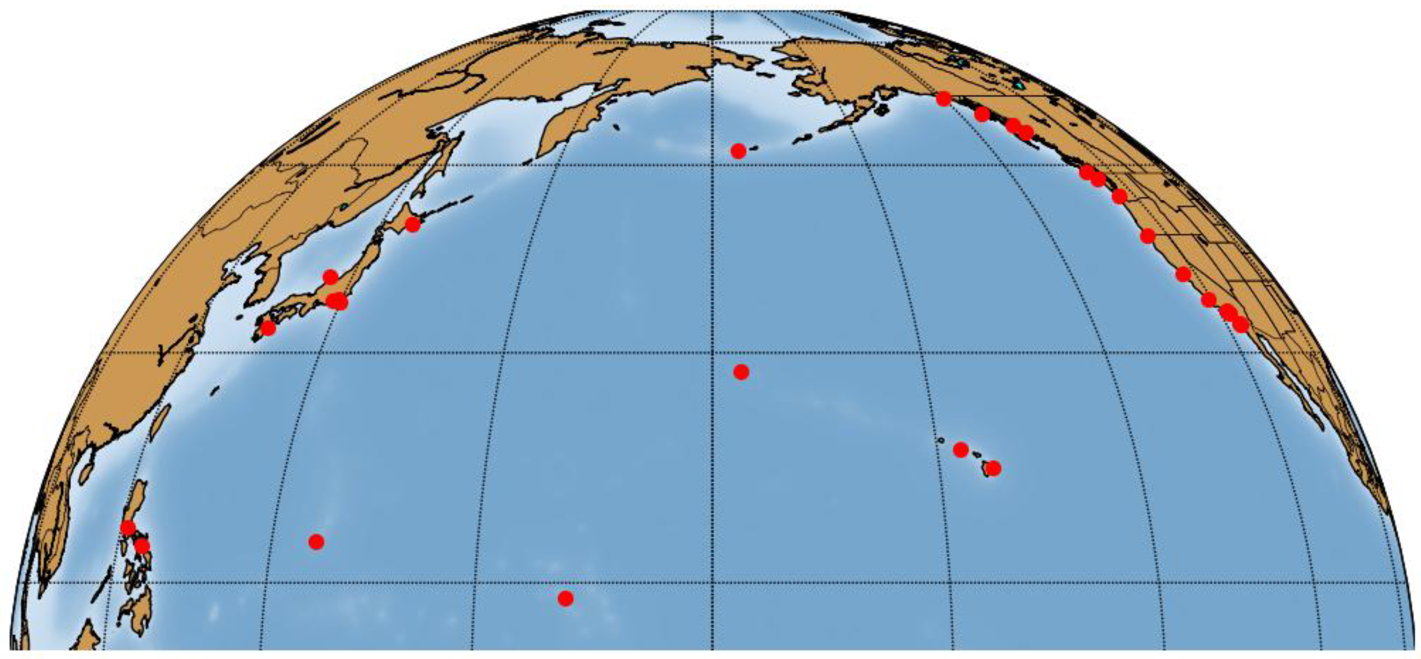
In the North Pacific region, the cross-correlation between stations is less clear due to the large distances between them. As noted above, when selecting predictors, it should be taken into consideration that there may be dependence between them. If large absolute values of cross-correlation coefficients (above 0.7–0.8) are found between some predictors, then one of the predictors should be excluded. The data from reference stations considered as candidate predictors should most fully reflect the climatic features of a large geographical region (information-homogeneous zone) and have long-term homogeneous observation series with a minimum number of gaps. In addition, reference stations should be located close to (or within) regions whose SST anomalies affect SAT anomalies at high and mid-latitudes [
26,
27]. Such a region in the North Atlantic is the tropical region (5.5° N–23.5° N, 15° W–57.5° W) [
51], where the Tropical Northern Atlantic (TNA) index is determined, and in the North Pacific it is the Warm Pool. The Key West and Manila Bay South Harbour tide gauge stations, located in the North Atlantic and North Pacific Oceans, respectively, meet these requirements.
In practice, however, a priori information useful for a reasonable selection of reference stations may often be lacking. A priori information may include, for example, estimates of the influence of anomalies in ocean characteristics (SST and/or SL) at low latitudes on atmospheric and oceanic heat transport to high latitudes and the formation of climatic anomalies in the Arctic and extratropics. In such cases, factor analysis and clustering can be used as a tool for selecting stations [
52,
53]. This implies, first of all, a structural analysis of the correlation matrix, which can be performed via principal component analysis. To this end, the SL data are detrended and normalized, and then a reduced correlation matrix is constructed. It may be recalled that a reduced correlation matrix is a matrix of pairwise correlations of observed variables. Its eigenvalues determine the fraction of each factor to common (total) variance allowing for the selection of a number of factors. At this stage, the factors that provide the largest proportion of cumulative variance are selected. In this context, factors are latent, cannot be measured directly, and are therefore hypothetical. The results obtained are used to form a factor loadings matrix. Its rows correspond to the original variables, and the columns correspond to the factors. At the intersection of a row and a column, the value of the loading is indicated, which represents the correlation coefficient between the original variable and the latent factor. Then, by applying hierarchical clustering to the factor analysis results, we can construct a connectivity matrix that can be visualized via a dendrogram.
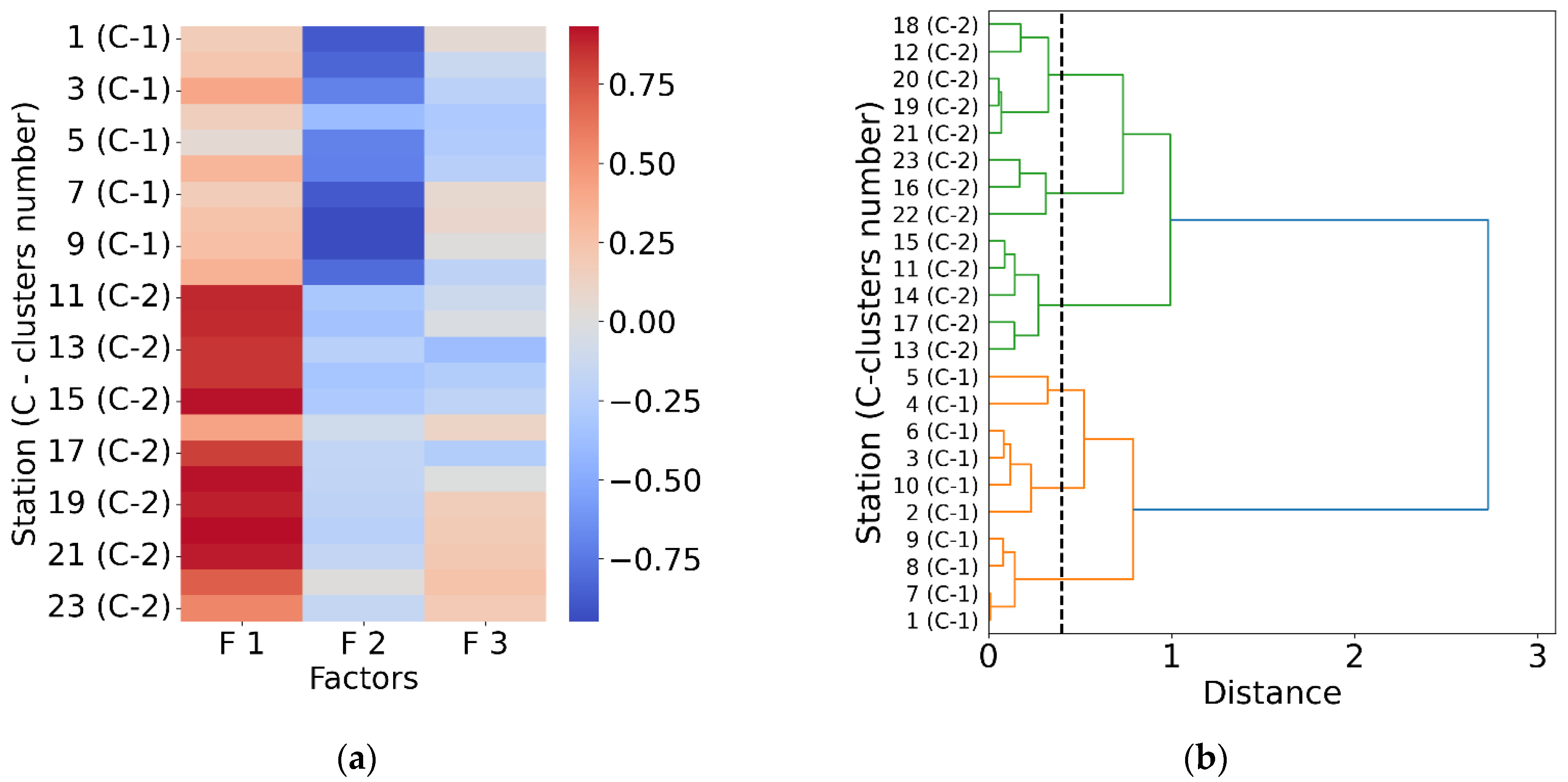
Table 4 presents the eigenvalues of the reduced correlation matrix, as well as the percentage of the total variance that is accounted for by each factor. The first two factors with eigenvalues of 12.89 and 4.19 determine the main patterns in the original data, explaining 74.2% of the total variance.
Figure 4a shows the factor loading matrix heat map, which provides a visual representation of the association of each factor with SL measured at each station. The largest contribution to the SL variance at stations 11–23 is made by the first factor, while the second factor is the most significant for stations 1–10. The third factor, not to mention other ones, makes the smallest contribution to the SL variance. The result of hierarchical clustering is visualized as a dendrogram and represented in
Figure 4b. This dendrogram shows two main clusters of stations. Cluster 1 is at the bottom and contains 10 stations (1–10), while cluster 2 is at the top and contains 13 stations (11–23). In total, the dendrogram has 6 levels. Stations of interest (1–5) located in tropical North Atlantic belong to cluster 1. All of these stations are root nodes, and each of them could theoretically be considered as a candidate for a reference station. However, all other things being equal, the proximity of the Key West tide gauge station to the “TNA” region and the completeness of its observation series are the determining factors in its selection as a reference station. The Key West station is located on the Florida Peninsula, near which the Florida Current merges with the Antilles Current, forming the Gulf Stream (at about 25° N). As is known, the Gulf Stream is part of the Atlantic Meridional Overturning Circulation (AMOC), which, in turn, affects the climate of remote regions located outside the North Atlantic, since it is part of the Broecker’s great ocean conveyor belt. Therefore, SL variations at Key West are a reliable indicator of variability in water circulation and various climate indices in the North Atlantic [
54].
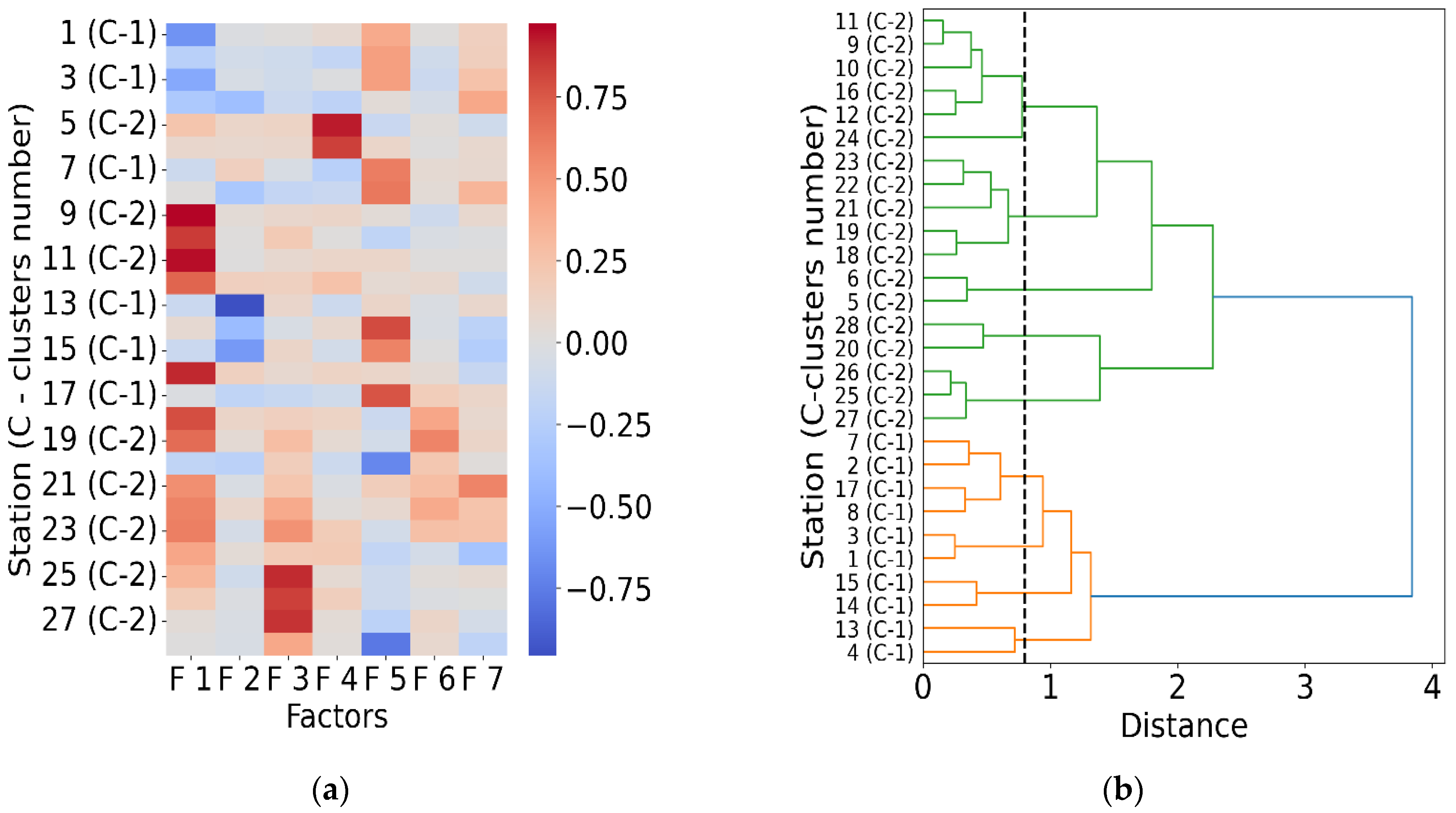
For the North Pacific Ocean, the situation is somewhat different. The eigenvalues of the reduced correlation matrix and the percentage of the total variance that is accounted for by each factor is presented in
Table 5 (for convenience’s sake, only data for factors 1–7 are included). Here, the first two factors explain more than 50% of the total variance. The corresponding heat map of the factor load matrix and dendrogram are shown in
Figure 5. The Manila Bay South Harbour tide gauge station, along with stations 1, 2, 3, and 7, belongs to cluster 1 and serves as the root node. It is the only station in the region with a long records and high data completeness (greater than 85%) and is located in the tropical Warm Pool. For these reasons, the Manila Bay South Harbour station was selected as the reference (candidate predictor) station for characterizing SL variations in the tropical North Pacific Ocean.
The Key West and Manila Bay South Harbour stations, selected as candidate predictors, are located in tropical regions where SSTs, as established earlier [
26,
27], influence SAT anomalies at high latitudes. The tropical North Atlantic region is defined as TNA (5.5° N–23.5° N, 15° W–57.5° W) [
38], while in the North Pacific Ocean, the relevant region is the Pacific Warm Pool Region (60° E–170° E, 15° S–15° N) [
55].
3.2. Variability and Links Sea Levels with Surface Air Temperature
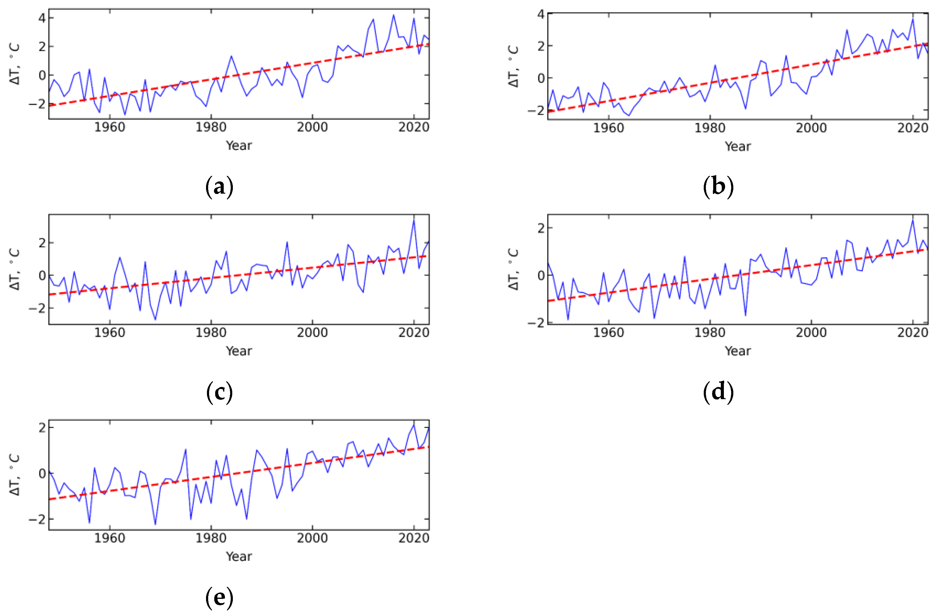
Further analysis requires information on how SATs changed from 1948 to 2023 in the five regions under consideration (see
Table 6 and
Figure 6). As is well known, since 1850, Earth’s temperature has increased by approximately 0.06 °C per decade, with the rate of warming accelerating to 0.26 ± 0.05 °C per decade over the past thirty years [
56]. It is therefore not surprising that regional SATs have also risen in recent decades, with the largest increases observed in the Arctic due to the Arctic amplification phenomenon. Indeed, over the past three decades, the Western Arctic has experienced the largest positive trend in annual average, increasing at a rate of 1.18 °C per decade, followed by the Eastern Arctic, and then Siberia and Europe (see
Table 6 for details).
As noted earlier, SST anomalies in the tropical North Atlantic and North Pacific, both exhibiting positive trends, have a time-lagged effect on SAT anomalies in mid- and high-latitude regions. This, along with other factors, support the assertion of a cause-and-effect relationship between tropical SST anomalies and SAT anomalies in these latitudes [
26,
27]. Since SL, like SST, shows a positive trend, and since the main drivers of SL increase are similar to those of SST, it is reasonable to assume a causal relationship also exists between rising SL in the tropics and the increase SAY in mid- and high-latitude regions.
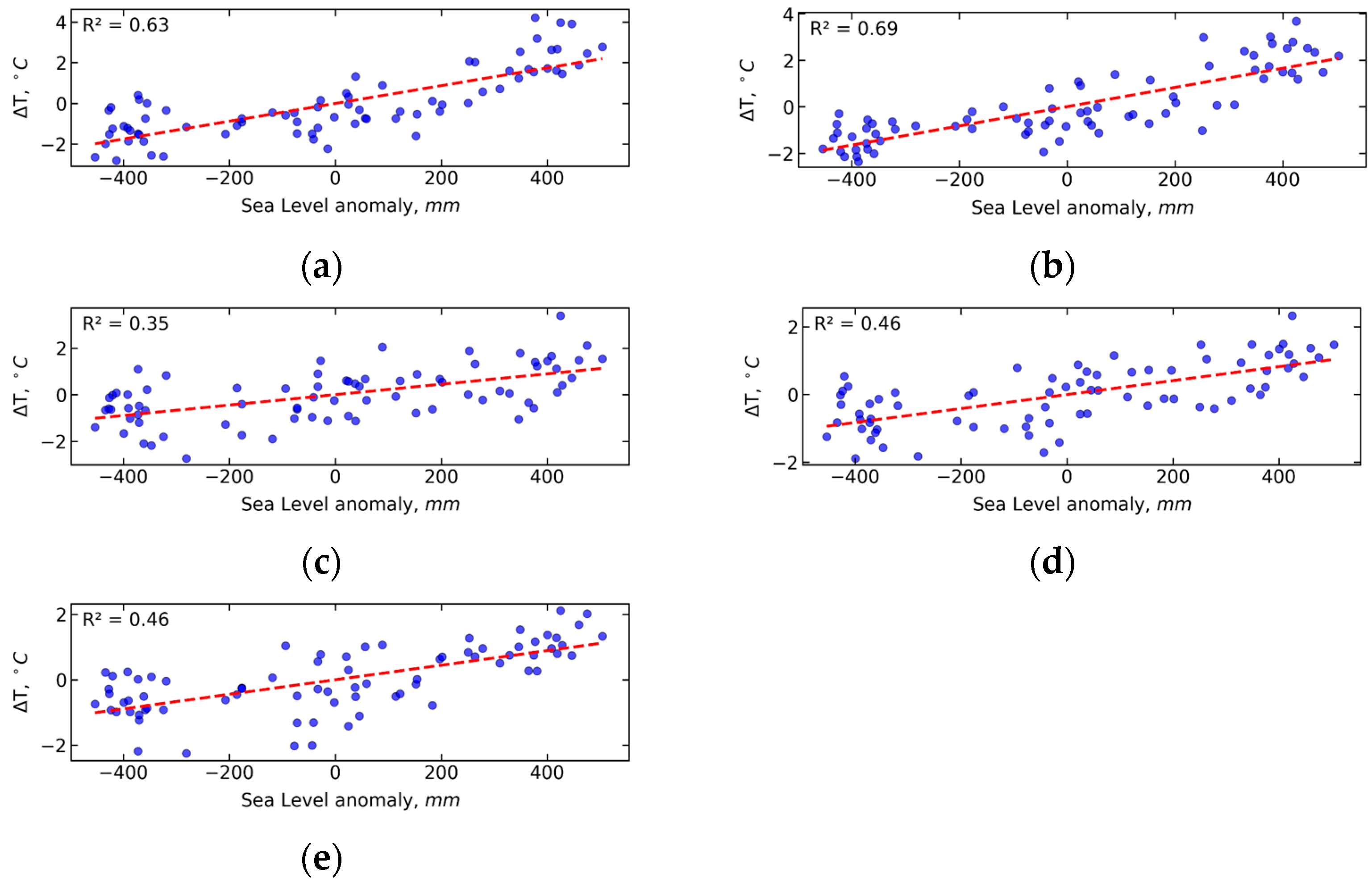
To explore the relationship between SL and SAT over the study period, scatterplots were generated and are presented in
Figure 7 and
Figure 8. The yearly average, time-unlagged correlation coefficient of approximately 0.80 indicates a strong positive linear relationship between SL anomalies in the tropical North Atlantic and tropical North Pacific SL anomalies and SAT anomalies in the Western and Eastern Arctic. A correlation coefficient of 0.75 between tropical North Atlantic SL anomalies and SAT anomalies in Eastern Europe also suggests a significant relationship. The linear relationship between tropical North Atlantic SL anomalies and SAT anomalies in Siberia is slightly stronger than that between tropical North Pacific SL anomalies and SAT anomalies in Siberia. SL variations in the North Atlantic also show a strong correlation with regional temperature changes (see
Figure 8 for details).
An analysis of correlations between annual mean SL in the tropics and annual mean SAT in various regions does not reveal a significant time lag between SL and SAT. However, time lag becomes evident when examining correlations based on seasonal and monthly mean data.
Table 7 presents the correlation coefficients among SST, SL, and SAT for the fall season, with the corresponding time lags indicated in parentheses. The focus on the fall season is based on previous findings [
26], which indicate that SST exerts its strongest influence on both SL and SAT during this period. As shown in
Table 7, the correlation coefficients between SL and SAT are comparable to those between SST and SAT, supporting the potential use of SL use as an indicator and predictor of climate change. The reliability of these results is further supported by the consistency of the observed time lags with the following principle of transitivity:
, where
denotes the time lag between variables
and
.
Additional evidence supporting the reliability of SL as a potential predictor is the structural similarity in the variability of SL, SST, and SAT, as observed in their power spectra.
Figure 9 displays the power spectra for SL at Key West and SAT anomalies in the Eastern Europe, both calculated for the fall season. After detrending, spectral density maxima are observed at periods of approximately 48, 8, 4, and 2.2 years in both spectra. Similar peaks are also evident in the SST spectra. In
Figure 9, the
–axis represents the conditional frequency
, and the
–axis shows the normalized spectral density. The period of oscillation
related to the conditional frequency
by the equation:
.
To describe the relationship between SL in the tropical regions of the North Atlantic and Pacific Oceans and SAT in remote regions, a multiple linear regression model was constructed. Sea level measurements from the Key West and Manila stations were used as independent variables in the model. Formally, the model can be represented by the following equation:
where
is the SAT in the
i-th region,
and
are the SL at the Key West and Manila stations, respectively;
,
and
are the regression coefficients, and
is the random error term.
Table 8 presents the values of the coefficients of determination and the standard errors of the regression model calculated for the five regions under consideration. The table shows that the coefficients of determination calculated for the Western and Eastern Arctic are significantly higher than those for the other regions. As is well known, the coefficient of determination is a measure of the quality of the forecast obtained using a regression model. Thus, it can be concluded that the regression model best explains the variability of SAT in the Arctic due to SL fluctuations in the tropics.


