1. Introduction
As global warming worsens, countries around the world are paying increasing attention to controlling greenhouse gas emissions. Effective monitoring of greenhouse gases is the primary issue to be faced in achieving global environmental governance and green and low-carbon development. Optical remote sensing technology, with its high scalability, sensitivity, and wide target detection characteristics, has obvious advantages in greenhouse gas monitoring and has become an important direction for the development of environmental monitoring technology. In atmospheric optical remote sensing technologies, spectral methods are primarily used for gas measurements [
1]. The core principle of spectral methods is based on the Beer–Lambert law, which states that the absorption of light is proportional to the concentration of matter and the length of the optical path [
2]. As light passes through the atmosphere, it is absorbed by trace gases in the atmosphere, causing the intensity of the light to decrease. By measuring the changes in the intensity of the light before and after it has passed through the atmosphere, the concentration of trace gases in the atmosphere can be inferred from the spectral information [
3]. Therefore, the key to effective atmospheric monitoring through optical remote sensing lies in how to accurately obtain the spectral information of gases.
Spatial heterodyne spectroscopy is a new type of spatially modulated Fourier interference spectroscopy technology that can achieve ultra-high spectral resolution within a determined spectral range [
4,
5,
6,
7,
8,
9]. Concurrently, it has the advantages of no moving parts, compact size, light weight, and relatively high sensitivity. It possesses distinctive advantages in applications such as atmospheric remote sensing, astronomical observation, and ore detection and has attracted considerable interest from scientists globally [
10,
11,
12]. The spatial heterodyne spectrometer modulates the light with detection target information into the spatial heterodyne interferogram. The interferogram can be processed into target spectral information, and this information processing is called spectral reconstruction. In the current algorithm, spectral reconstruction requires a series of information processing processes such as baseline removal, apodization, Fourier transform, and calibration [
13]. Complex information processing means that spectra may suffer additional data loss. With the increasing demand for spectral accuracy in optical remote sensing monitoring technology for pollution control and carbon reduction, how to simplify the spectral reconstruction process in spatial heterodyne spectroscopy and improve spectral accuracy is an urgent research problem.
In the past decade, the rapid development of deep learning has brought new solutions to research difficulties in different fields [
14,
15,
16]. In the field of optical information processing, the regression prediction method of deep neural networks is an important research direction. The method fits inputs and outputs by building a neural network to learn their hidden relationships from a large number of data samples of inputs and outputs, adjusting the parameters with feedback, to establish a nonlinear implicit mapping relationship. This research has made rapid progress in the optimization design of micro–nano-devices [
17,
18,
19] and spectral prediction [
20,
21,
22,
23] and has achieved remarkable results [
24,
25]. However, there are few reports in the field of spectral reconstruction for spatial heterodyne spectroscopy.
In atmospheric remote sensing using a spatial heterodyne spectrometer, wavelength bands are typically chosen where only the target gas exhibits significant light absorption, in order to eliminate interference from other gaseous factors. Consequently, the resulting spectral shapes are relatively fixed, with variations in intensity occurring mainly at specific wavelengths [
26,
27]. It can also be understood that some spatial heterodyne spectrometers are designed specifically for spectral detection of particular targets. Due to the precise definition of the detection goals, the spatial heterodyne spectrometer can be engineered with very narrow detection bands, thereby achieving sub-nanometer-level ultra-high spectral resolution [
4,
5,
6,
7,
8,
9]. This capability represents the core competitive advantage of spatial heterodyne spectrometers. Therefore, the spectral reconstruction of specific detection targets by spatial heterodyne spectrometers can also be achieved using regression prediction methods based on deep neural networks.
This paper adopts deep learning to study the spectral reconstruction method of specific spatial heterodyne interferograms, building a deep neural network to learn the mapping relationship between the interferometric information of spatial heterodyne interferograms and spectral information. The ultimate goal is to simplify the processing process from spatial heterodyne interferograms to spatial heterodyne spectra and improve spectral accuracy. The results are expected to provide a new solution for extracting spatial heterodyne spectral information from specific spatial heterodyne interferograms, which has potential applications in spectral reconstruction across multiple remote sensing platforms (ground, airborne, satellite, and so on) equipped with a spatial heterodyne spectrometer.
2. Models and Methods
Figure 1 shows the structure of a spatial heterodyne spectrometer. The optical path of the spatial heterodyne spectrometer is as follows: First, the light of the measured object passes through the aperture A of the pre-collimation system and the collimating lens L1. The lens L1 collimates the incoming light to form light parallel to the optical axis, which then enters the beam splitter through the incident wavefront. The beam splitter divides the incident light into two coherent beams with the same energy. The reflected light is directed towards the blazed grating G1, and the transmitted light is directed towards the blazed grating G2. After diffraction by the blazed grating, the two parts of the light are directed towards the beam splitter again. Due to the different angles of the two phases of coherent light (reflected and transmitted light after grating diffraction) emitted, spatial interference fringes are generated on the output wavefront, and finally, the spatial heterodyne interferogram appears on the CCD [
27]. When the incident light spectrum is
, the spatial heterodyne interferogram can be represented as follows:
Here,
is the interference intensity,
is the grating diffraction direction,
is the wavenumber,
is the Littrow wavenumber, and
is the Littrow angle [
27].
The optical path difference of coherent light is set as
. The expression for the modulation part of the spatial heterodyne interferogram obtained by substituting ∆ into Equation (1) is as follows:
According to the Fourier transform, the incident spectrum
is
Therefore, the spectral information
is the inverse Fourier transform of the interferometric information
. However, in practical measurements, the interferogram requires a series of data processing steps, such as apodization, before performing the Fourier transform [
28]. Thus, the key to spectral reconstruction lies in how to characterize and process the complex mapping between the spectral information
and the interferometric information
. Deep learning has significant advantages in handling complex and nonlinear mappings. Through training and learning from sample data, it can uncover the relationship between spectral information and interferometric information, thereby constructing high-precision reconstruction models. Therefore, deep neural networks can be utilized to address the problem of spectral reconstruction from specific spatial heterodyne interferograms.
The constructed deep neural network referenced from references [
17,
23] is shown in
Figure 2. Typically, each row of data in a spatial heterodyne interferogram contains similar interferometric information, and spectral reconstruction can be achieved by a single row of data. The number of nodes in the input and output layers of the network is consistent with the effective number of pixels in the image detector of the spatial heterodyne spectrometer. This design ensures that each network node in the input and output layers corresponds directly to a physical sampling unit of the detector, thus maintaining strict hardware matching. In this paper, based on subsequent simulation data and the parameters of the instrument in the laboratory, both are set to 1024. To ensure that the model has sufficient learning and information processing capabilities, while avoiding an overly complex network structure, the hidden layer is set to 5 layers, with 1024 nodes in each layer (maintaining dimensional consistency of information flow to avoid information loss or gradient anomalies caused by sudden changes in dimensions), and a fully connected approach is adopted. The number of hidden layers and nodes can be adjusted according to specific needs based on different instruments and spectral reconstruction tasks.
activation functions are added between each layer to increase the network’s nonlinear capability while reducing computational complexity and solving gradient vanishing problems. The learning rate is set to 0.00001. The transformation process of deep neural networks can be expressed as
Here, ω is the weight, is the bias term, is the activation function, and is the output.
represents the trained network. The spectral reconstruction for specific spatial heterodyne interferograms based on the deep neural network can be expressed as
In order to evaluate the effectiveness of the neural network objectively, the
(Mean Square Error) [
29] and
(Coefficient of Determination) [
30] were selected to evaluate the trained model. Meanwhile, the
(Mean Absolute Error) [
31] was used to characterize the spectral difference between the predicted spectrum and the target spectrum. The formulas are as follows:
Here, is the predicted spectrum, is the target spectrum, is the mean of all target spectra, and is the number of samples. The closer the and are to 0, the closer is to 1, indicating a better fit between the predicted and target spectra.
3. Results and Discussion
To verify the effectiveness of the spectral reconstruction method for specific spatial heterodyne interferograms based on deep neural networks, 2400 sets of CO
2 radiative spectra were calculated using the SCIATRAN radiative transfer model [
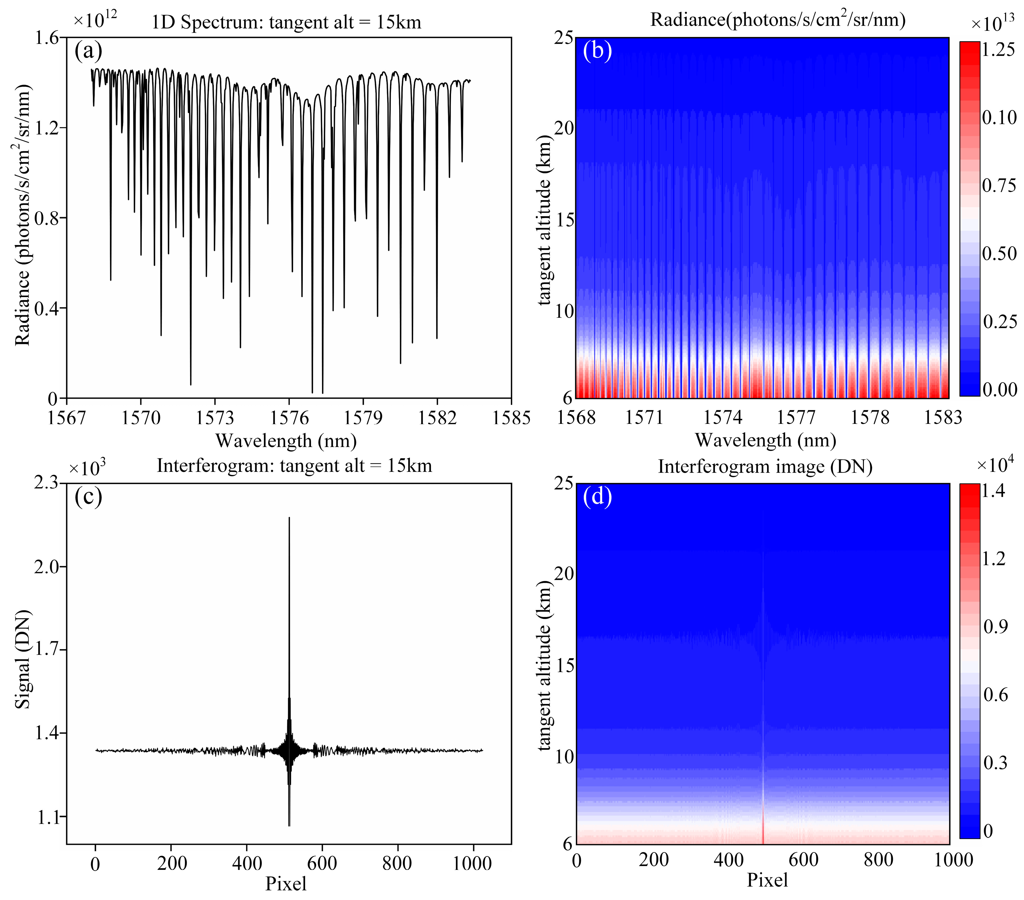
32]. The calculations were performed under different observational geometry and parameter conditions, with an altitude range of 6–25 km, a wavelength range of 1568–1583.3 nm, and a spectral resolution of 0.03 nm. Among them, the CO
2 radiation spectrum at a zenith angle of 60 degrees, a relative azimuth angle of 45 degrees, and an altitude of 15 km is shown in
Figure 3a.
Figure 3b displays the CO
2 radiation spectra within the altitude range of 6–25 km. It is clearly observed that at lower altitudes, the radiation brightness is higher, and as the altitude increases, the radiation brightness gradually decreases. According to the theoretical framework of spatial heterodyne spectroscopy proposed by Harlander [
4] (Equation (1)), and the 2400 sets of CO
2 radiative spectra computed by the SCIATRAN radiative transfer model serving as the incident spectra, the corresponding 2400 sets of spatial heterodyne interferometric data can be simulated.
Figure 3c presents the simulated interferometric data for the CO
2 radiative spectrum shown in
Figure 3a, while the interferometric data across the altitude range of 6 to 25 km are depicted in
Figure 3d. It is apparent that the intensity of the interference varies significantly with the changes in radiance at different altitudes.
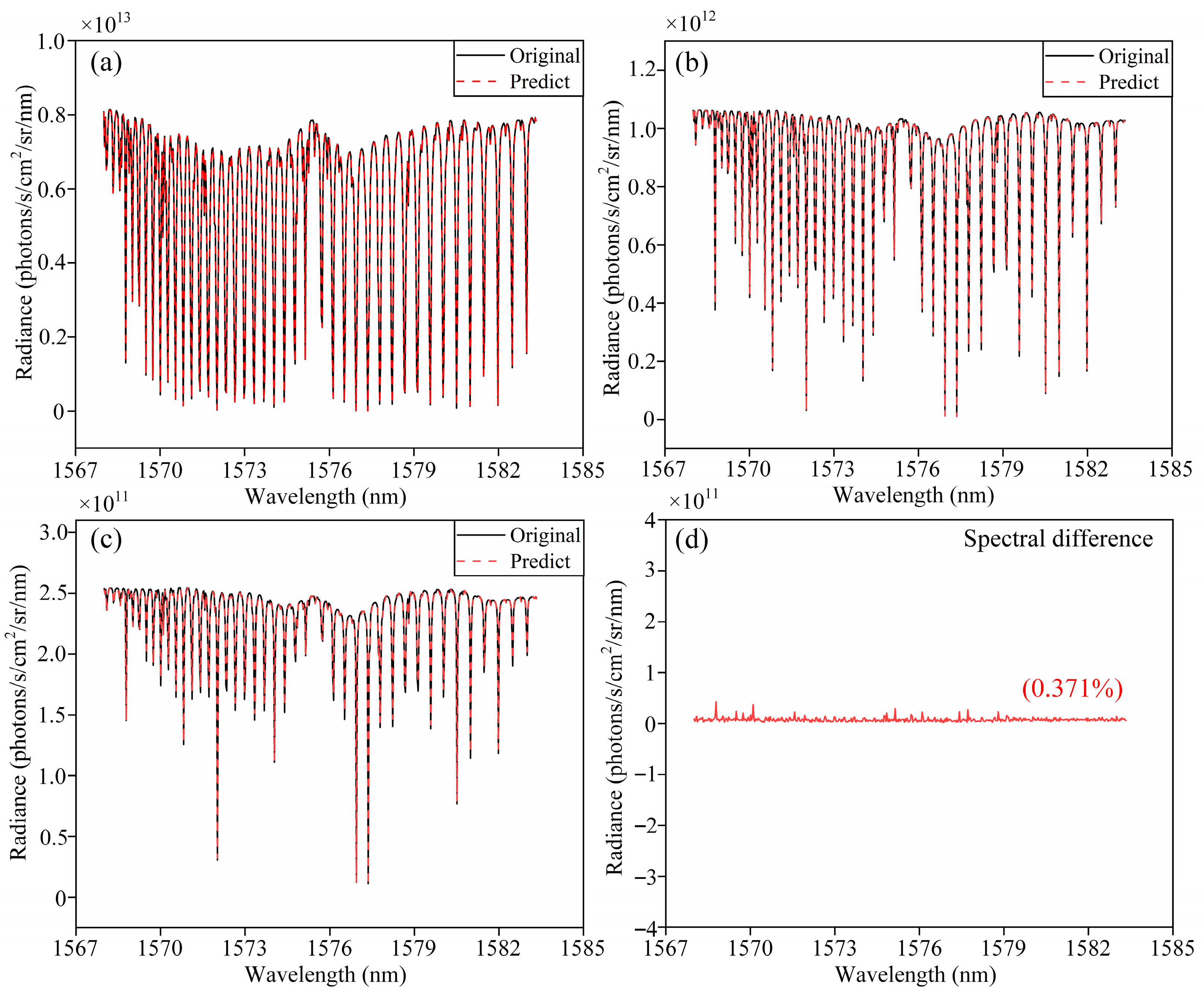
A random selection of 2100 sets of CO
2 interferometric information and their corresponding radiative spectra were used as the training set to train the constructed deep neural network. The trained spectral reconstruction deep neural network model is referred to as SRDNN. The remaining 300 sets of CO
2 interferometric information were used as the test set. Three sets of CO
2 interferometric information with varying intensities were randomly selected from the test set and input into SRDNN. The CO
2 predicted spectra from SRDNN and the target spectra are shown in
Figure 4a–c. As can be seen from the figures, the CO
2 spectra at different intensities predicted by SRDNN closely overlap with the target spectra, and the intensities of the spectral absorption peaks are also very similar. All interferometric information in the test set was input into SRDNN, and the average
between the predicted spectra and the target spectra reached 0.9943, with an average
of 0.00021.
Figure 4d shows the average spectral difference between all predicted spectra and target spectra in the test set. The spectral line approximates a straight line, with only minor fluctuations present. This result indicates that the CO
2 predicted spectra are nearly identical to the target spectra, demonstrating that the spectral prediction performance of SRDNN is highly satisfactory. It preliminarily validates the effectiveness of the spectral reconstruction for specific spatial heterodyne interferometric information based on deep neural networks.
To further study the effectiveness and universality of the spectral reconstruction method for specific spatial heterodyne interferograms based on deep neural networks, this study also validated the method using experimental data.
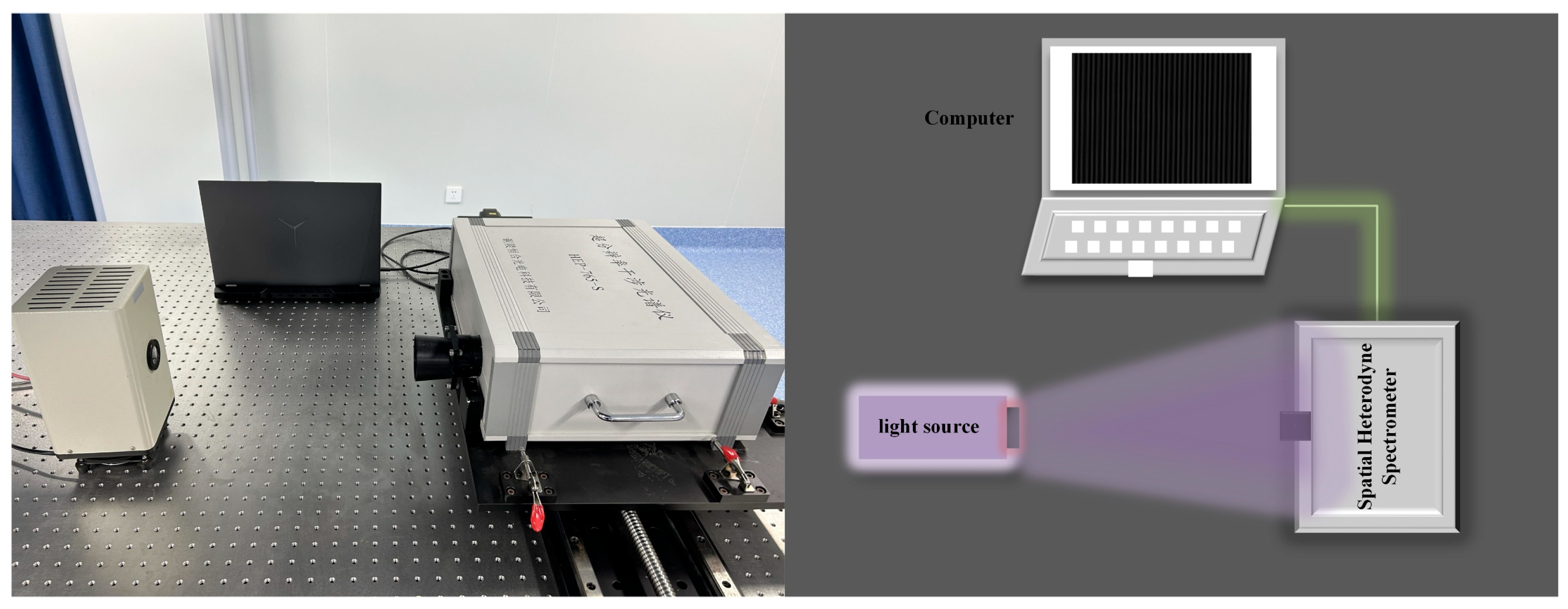
Figure 5 shows the experimental instrument used for data collection in this study and its optical path schematic. As shown in the figure, the experimental setup mainly consists of a light source, a spatial heterodyne spectrometer, and a computer. The internal optical path structure of the spatial heterodyne spectrometer is shown in
Figure 1. The main performance parameters of the spatial heterodyne spectrometer used in this experiment are a spectral range of 756–771 nm and a spectral resolution of 0.03 nm. The light emitted by the light source is collected by the spatial heterodyne spectrometer and modulated into a spatial heterodyne interferogram by its internal optical path, which is ultimately stored by the computer.
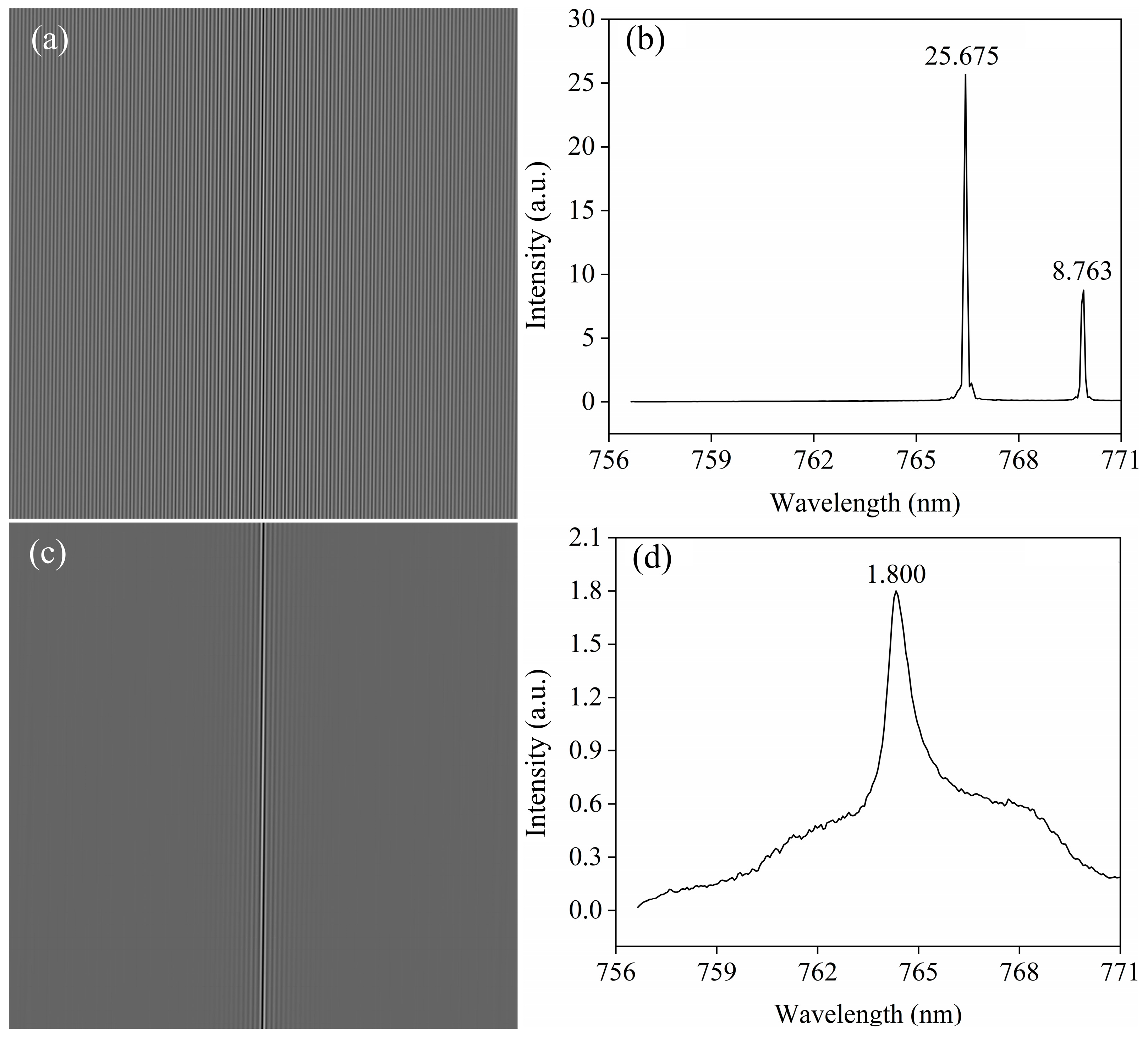
Based on the actual experimental conditions, and in order to meet the research requirements, this paper used a potassium lamp (wave peaks: 766.5 nm and 769.9 nm) and a xenon lamp (spectral range: 200–2500 nm) as light sources to collect 2400 spatial heterodyne interferograms with different intensities using the spatial heterodyne spectrometer. Due to the limitations of the experimental conditions, the original spectra of the potassium lamp and xenon lamp could not be obtained. Therefore, the spatial heterodyne spectra after Fourier transform of the spatial heterodyne interferograms were used as the target spectra to validate the effectiveness of the method. In total, 2100 sets of data were randomly selected from the potassium lamp and xenon lamp datasets, forming a mixed training set of 4200 sets of interferometric and spectral data. The remaining 300 sets from each were used as the test set.
Figure 6a,c show the interferograms of potassium and xenon lamps randomly selected from the test set, respectively. Extracting interferometric data from the potassium lamp interferogram, the converted spectrum is shown in
Figure 6b, with peak values of 25.675 and 8.763 at 766.5 nm and 769.9 nm, respectively. The corresponding spectrum of the xenon lamp interferogram is shown in
Figure 6d, with a peak of 1.800 at 764.3 nm.
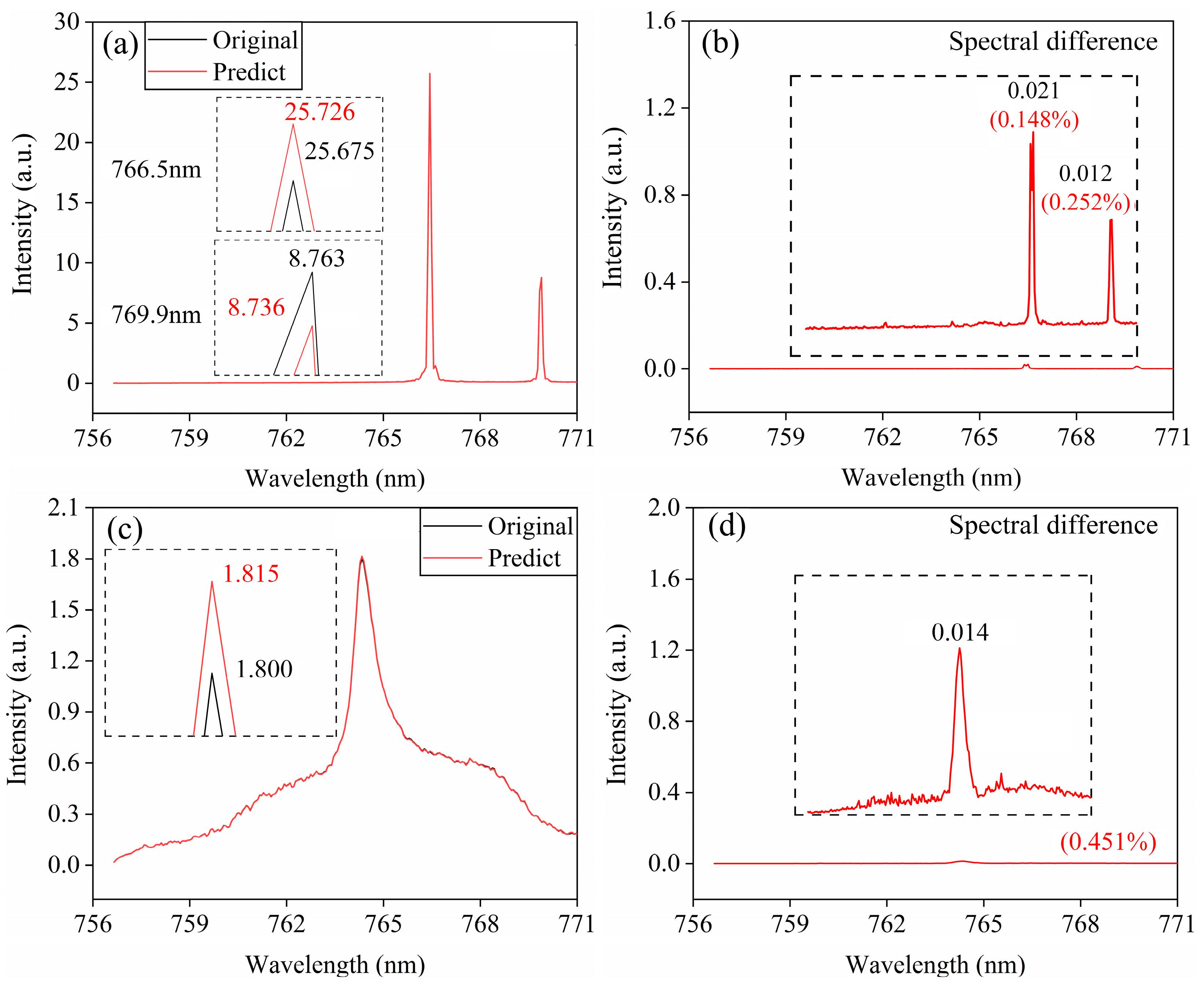
Importing the above mixed training set into the constructed deep neural network for training, the trained SRDNN-S is a spectral reconstruction model specifically for interferometric information from potassium and xenon lamps. The predicted spectrum and the target spectrum of the randomly selected potassium lamp spatial heterodyne interferogram are shown in
Figure 7a. It can be observed from the figure that the predicted spectrum closely matches the target spectrum, with only minor differences in the peak. The interferometric information from the 300 potassium lamp spatial heterodyne interferograms in the test set was input into SRDNN-S. The average
between the predicted spectra and the target spectra was 0.9986, with an
of 0.0000093238. In
Figure 7b, the average difference between the predicted spectra and the target spectra for all potassium lamp interferograms in the test set was 0.021 at 766.5 nm, which is 0.148% of the average target spectral peak, and 0.012 at 769.9 nm, which is 0.252% of the average target spectral peak.
The predicted spectrum and the target spectrum of the randomly selected xenon lamp spatial heterodyne interferogram are shown in
Figure 7c. From the figure, it is evident that the xenon lamp predicted spectrum and the target spectrum also exhibit a high degree of overlap. In the magnified comparison view, the predicted spectral peak is 1.815, differing from the target spectral peak by 0.015. The interferometric information from the 300 xenon lamp spatial heterodyne interferograms in the test set was input into SRDNN-S. The average R
2 between the predicted spectra and the target spectra was 0.9987, with an MSE of 0.0000137640.
Figure 7d shows that the predicted spectral peak for the xenon lamp in the test set differs from the target spectral peak by an average of 0.014, while the average spectral difference across the entire spectral line accounts for only 0.451% of the original spectral line. The results of spectral prediction by SRDNN for both potassium and xenon lamp spatial heterodyne interferograms indicate that the spectral reconstruction method for specific spatial heterodyne interferograms based on deep neural networks also exhibits excellent spectral reconstruction capability for the experimental data. This further proves the effectiveness and universality of the method.
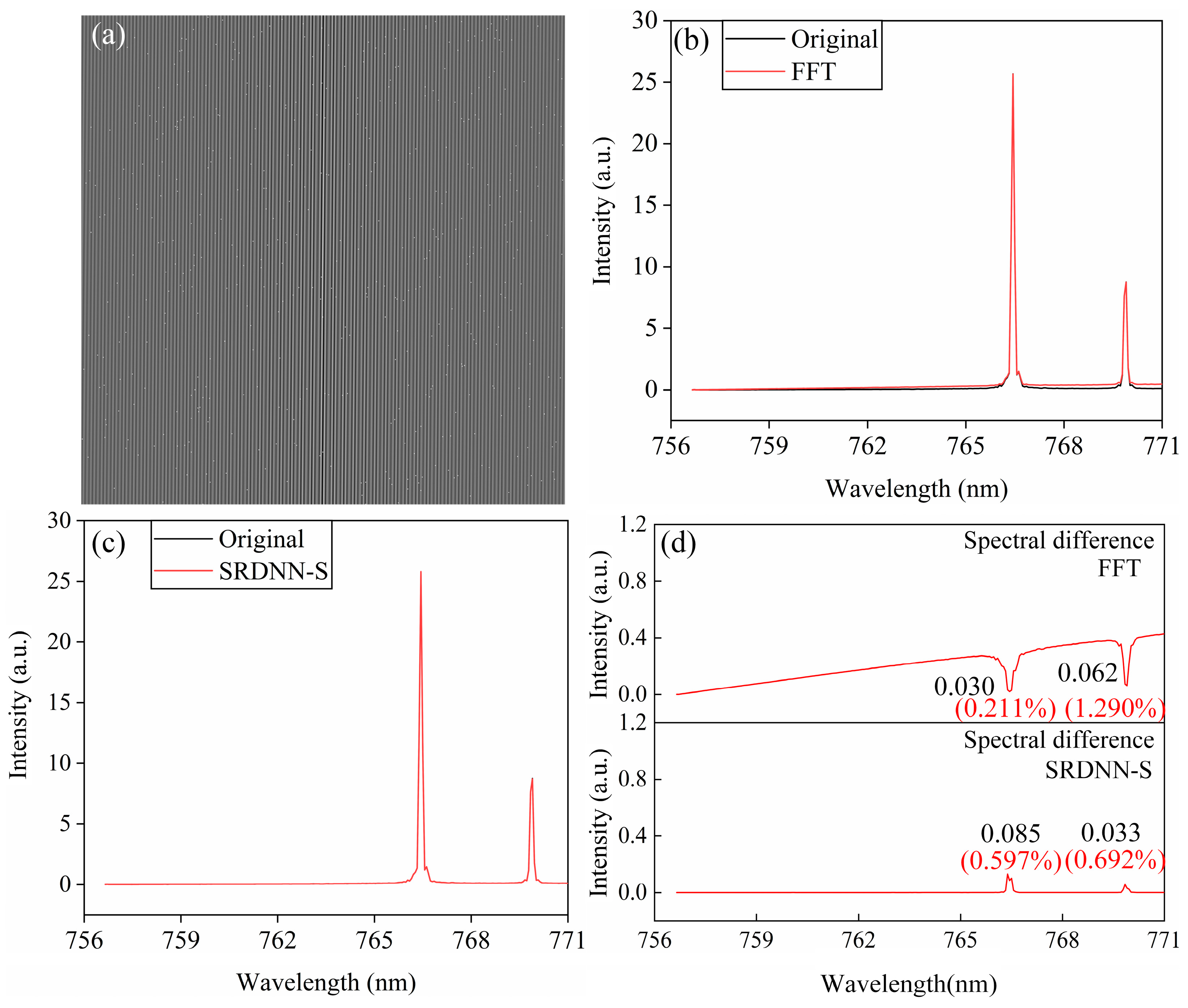
Furthermore, this paper investigates the robustness of the spectral reconstruction method of specific spatial heterodyne interferograms based on deep neural networks. Random 0.1% bright spot noise was added to all the potassium lamp spatial heterodyne interferograms in the test set. A representative noisy potassium lamp interferogram is shown in
Figure 8a, where it can be observed that the interferogram is slightly affected by noise. Without denoising, the noisy interferogram was processed using FFT (Fast Fourier Transform) and other information processing techniques. The reconstructed spectrum shows a certain discrepancy compared to the original noiseless spectrum, as shown in
Figure 8b. In contrast, after SRDNN-S performs spectral reconstruction on the noisy interferogram, the reconstructed spectrum is almost unaffected by noise and highly similar to the original noiseless spectrum, as shown in
Figure 8c.
Figure 8d shows the average spectral difference between the reconstructed spectra (using FFT and SRDNN-S) and the original noise-free spectra for all noisy potassium lamp interferograms in the test set. The figure clearly shows that the FFT difference spectrum displays much more pronounced fluctuations than the SRDNN-S difference spectrum. At both spectral peaks, SRDNN-S maintains an average spectral difference below 0.7%, while FFT yields a 1.290% difference at a 769.9 nm wavelength. These results preliminarily demonstrate that the spectral reconstruction method of specific spatial heterodyne interferograms based on deep neural networks possesses certain interference-resistant capability and can reliably reconstruct accurate spectral information.
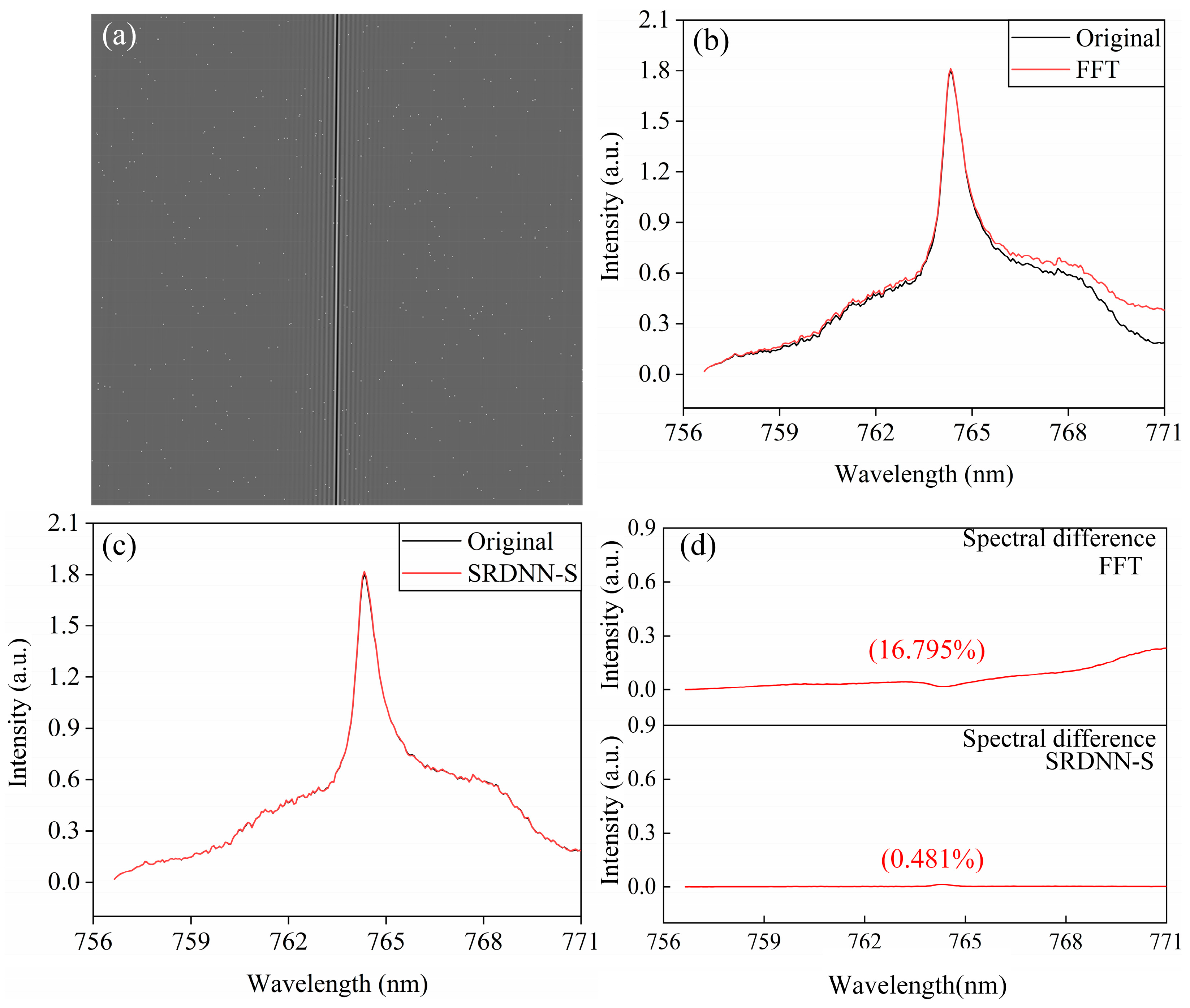
Random 0.1% bright spot noise was added to all the xenon lamp spatial heterodyne interferograms in the test set. A representative noisy xenon lamp interferogram is shown in
Figure 9a. Without denoising, the reconstructed spectra obtained by FFT and SRDNN-S are shown in
Figure 9b and
Figure 9c, respectively. As observed in
Figure 9b, the spectrum reconstructed by FFT shows significant deviations from the original noiseless spectrum, while in
Figure 9c, the spectrum reconstructed by SRDNN-S demonstrates excellent agreement with the noiseless spectrum.
Figure 9d shows the average spectral difference between the reconstructed spectrum and the original noiseless spectrum after spectral reconstruction of all noisy xenon lamp spatial heterodyne interferograms in the test set using FFT and SRDNN-S. The xenon lamp is a continuous spectral light source; its spatial heterodyne interferograms contain broad spectral information, making them more sensitive to noise. Therefore, after FFT transformation, the average spectral difference in the noisy and noiseless xenon lamp interferograms reaches 16.795%, while SRDNN-S retains a lower average spectral difference of 0.481%. These results further demonstrate that the spectral reconstruction method of specific spatial heterodyne interferograms based on deep neural networks exhibits certain stability and noise immunity. In the case of interferograms with slight noise, SRDNN-S can accurately reconstruct the spectrum without additional data processing, which simplifies the spectral reconstruction process to some extent compared to the FFT spectral reconstruction method.
It is worth noting that the spectral reconstruction method based on deep neural networks has the ability to reconstruct the spectra of the specific spatial heterodyne interferograms after fully training a large amount of data obtained by a specific spatial heterodyne spectrometer (for the specific target), but it has no spectral reconstruction effects on interferograms of other untrained elements or gases. Therefore, FFT is still the mainstream spectral reconstruction method, and deep neural networks currently cannot replace the universal applicability of FFT.

