Solar and Wind 24 H Sequenced Prediction Using L-Transform Component and Deep LSTM Learning in Representation of Spatial Pattern Correlation

Abstract

Spatiotemporal correlations between meteo-inputs and wind–solar outputs in an optimal regional scale are crucial for developing robust models, reliable in mid-term prediction time horizons. Modelling border conditions is vital for early recognition of progress in chaotic atmospheric processes at the destination of interest. This approach is used in differential and deep learning; artificial intelligence (AI) techniques allow for reliable pattern representation in long-term uncertainty and regional irregularities. The proposed day-by-day estimation of the RE production potential is based on first data processing in detecting modelling initialisation times from historical databases, considering correlation distance. Optimal data sampling is crucial for AI training in statistically based predictive modelling. Differential learning (DfL) is a recently developed and biologically inspired strategy that combines numerical derivative solutions with neurocomputing. This hybrid approach is based on the optimal determination of partial differential equations (PDEs) composed at the nodes of gradually expanded binomial trees. It allows for modelling of highly uncertain weather-related physical systems using unstable RE. The main objective is to improve its self-evolution and the resulting computation in prediction time. Representing relevant patterns by their similarity factors in input–output resampling reduces ambiguity in RE forecasting. Node-by-node feature selection and dynamical PDE representation of DfL are evaluated along with long-short-term memory (LSTM) recurrent processing of deep learning (DL), capturing complex spatio-temporal patterns. Parametric C++ executable software with one-month spatial metadata records is available to compare additional modelling strategies.

1. Introduction

Accurate forecasting of solar and wind output is essential for effective load planning, resource allocation, and stability in RE-based autonomous systems. Advanced AI statistical methods improve the management of detached smart grids in coastal, remote, or desert areas, ensuring optimal operation. It is necessary to estimate the production capacity of photovoltaic (PV) plants and wind farms adequately, considering the configuration specifics and user demands, to stabilise the power supply. Inherent variability in solar and wind parameters under specific atmospheric and ground surface local formations can result in insufficiency in conventional simulations or operable stand-alone solutions in a day-horizon. Integration of AI methodologies based on statistical pre-analysis takes advantage of better accessibility compared to traditional regression or physical approaches. Advanced AI tools support the broader use and transition to sustainable energy, which is important in remote areas and developing countries [1]. AI statistics using large data archives can provide simple analytical solutions, independent of long-term physical and time-consuming numerical simulations, and improve their results [2]. Contrary to AI-independent computing, in numerical weather prediction (NWP), a lower spatial resolution has a greater temporal validity, although a higher spatial resolution in computed parameters leads to a decrease in the related temporal scale. These systems simulate the evolution processes in the atmosphere according to the physical laws, using a standard definition scale. The NWP output on a lower temporal scale is generally related to short-term forecasting [3]. Simulation costs and demands require intensive supercomputing, determining the applicability of NWP in long-term forecasting on large scales [4]. One of the main disadvantages of physical systems is the need for observations from several atmospheric layers. NWP systems use exact mathematical equations to approximate the 3D progress of each reference parameter. Solar and wind data can be directly transformed into power produced in photovoltaic plants or wind farms according to defined operational characteristics that relate the output to forecasts [5]. Unaccommodated large-scale NWP outcomes are considerably delayed by a few hours (due to computation costs). Their AI conversions underline possible NWP inaccuracies in undetermined terrain asperity and system design [6]. The AI-tuned models are fully adapted to the variability of local patterns and the configuration of energy production systems from available training databases. Despite efficiency, self-contained AI computing may fail in longer predictive horizons of unexpected frontal disruptions, not indicated in the data sets [7].

The proposed AI-based statistical prediction starts with identifying optimal data sequences necessary to capture dynamic complexity in long-term self-contained modelling. Various approaches to data sampling and partitioning can be found in the literature (Section 2). In this study, historical data series are processed sequentially to identify initialisation times related to the last observational changes. Recognised training intervals are re-evaluated secondarily according to the pattern similarity. Integrating correlation statistics in training data refinement yields better representation of predictive relevant patterns, significantly implying model reliability and stability for unknown input. The correlation characteristics reveal recent changes in the atmosphere that primarily affect the calculation of the target output in estimate periods [8]. The hybrid nature of the proposed binary node PDE modelling framework facilitates pattern differentiation in soft computing. Its modular concept is based on adapted PDE re/transformation procedures of Operation Calculus (OC) applied in solving node-defined separable PDEs in evolutionarily formed binomial networks. A tree-like structure, based on the GMDH design (Group Method of Data Handling) [9], decomposes the general differential expression of a dynamical system described by data samples into a separable set of PDE node solutions using OC. The architecture can be extended by a complex-valued neural network (CNN) that allows the processing of double amplitude/phase information [10]. Phase or angle input (wind, radiation, etc.) is combined with the amplitude data representing the pattern cycles in periodical substitution for determined node PDEs in complex form.

The applied day-ahead selective modular PDE modelling includes the following (Section 4):

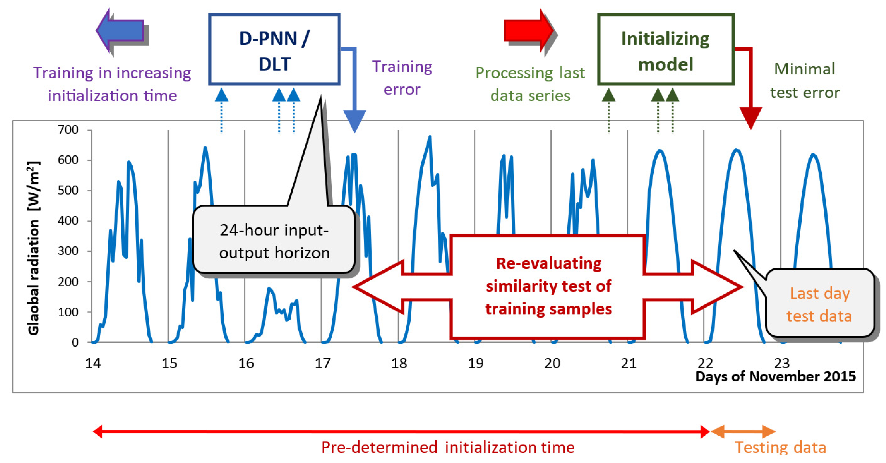
• First identification of model initialisation times in applicable data periods.
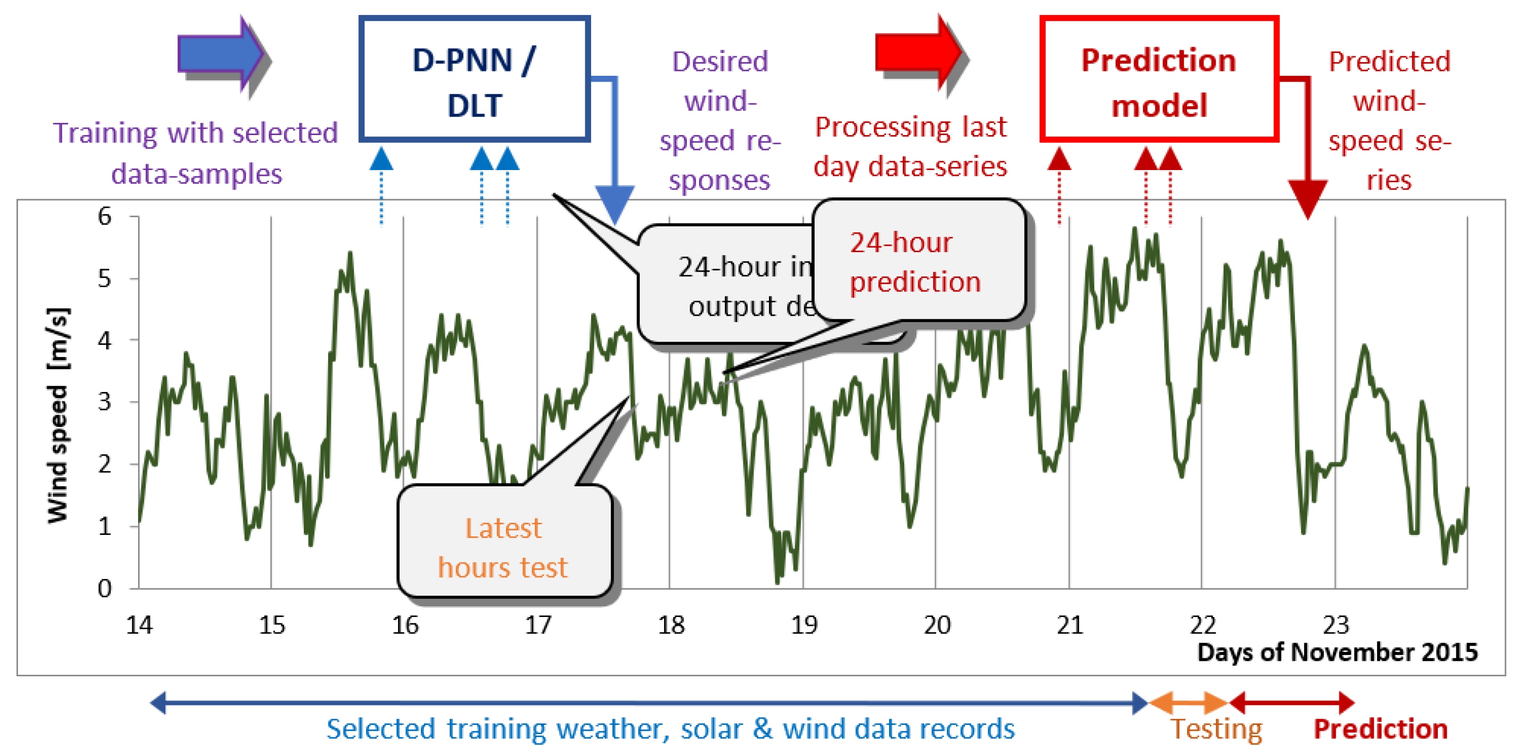
• Sampling of detected training intervals based on similarity parameters.
• Evolutionarily produced PDE components related to the pattern complexity.
• Self-combination of the most valuable node double inputs in a tree-like structure.
• PDE node transformation and inverse solution based on adapted numerical procedures.
• Optimisation of the network structure and the combinatorial selection of PDE modules.
• Assessment of the testing model in the final computing stage.

2. State of the Art in Solar and Wind Series Daily Similarity Prediction

Multiple AI strategies emphasise the use of feature selection, transformation, or analysis based on pattern characteristics in the first data evaluation before training [11]. Hybrid methodologies fuse various recently designed machine learning (ML) and novel pre-processing techniques to improve segregate modelling analogous to the presented hybrid neuro-numerical approach (Section 4). The inherent character of wind and solar series can be suppressed by the hyperparametric wavelet transform using spectral analysis to optimise the order of functions and trend ratio parameters in pre-processing [12]. Discrepancies in the raw data can be revealed by a boxplot re-analysis based on interpolation of the kriging components. The clustering of informal input, which allows the modelling of patterns on multiple scales, organises the data by evaluating the efficiency of training [11]. Evaluating correlations between near-Earth solar–wind large-scale factors can significantly enhance predictability in day cycles analogous to the applied spatial similarity index (Section 3). Optimal identification of relevant local-type conditions improves cascade forecasting on a day-horizon [13]. Empirical decomposition combined with metaheuristics can help identify initialising parameters and multivariate limitations in forecasting times to reduce uncertainty. Autoregressive modelling based on variational decomposition addresses the relationship of long-term patterns in chaotic fluctuation [14]. Separation of data components and deposition increase the accuracy of hybrid modelling. Spatial and temporal data can first be analysed to capture complex interactions between different variables [15]. Constraint theory integrated with quasi-Newton formulas improves learning by separating characteristics in data sequences [16]. Integrating AI with physics-based methods based on different problem solutions improves the reliability of probabilistic prediction [17]. Solar data can be converted with photovoltaic power curves on a long-term horizon, although radiation forecast is usually missing from standard free available local NWP supplies [11]. Field re-analysis, generated by a global NWP system, can identify the most important predictors related to solar and wind output, supplemented by the characteristic components grouped into sets [18]. The correlations between the NWP series and the clarity factors can be revealed to correct the original irradiance forecast [19]. Forecast errors can exceed 20% for 24 h NWP, highlighting the need for operational resource reallocation and planning to accommodate such uncertainties. Data-driven fusion stack-ensemble learning, which captures the frequent short-term fluctuations inherent in RE, can use the long-short-term memory (LSTM) frame of DL, with the ability to represent long-temporal spatial relations [4]. LSTM memory cells maintain information for extended time intervals, evaluated in Section 6, representing specific seasonal trends in historical sets necessary in strategic planning [20,21]. Enhanced DL in solar forecasting can include feature engineering using kernel component analysis prior to LSTM training based on time-of-day mode classification for historical and NWP data in error correction post-processing [22]. Granular analysis allows Gaussian regression to learn complex patterns more effectively in stepwise component prediction. Meteorological data can be transformed into specific wave components to reconstruct variables in the predictive model. Estimation of the backup state of charge (SoC) with load demands is essential in microgrid energy management [1]. Detailed pattern analysis combined with optimal ensemble voting improves probabilistic quantile regression in RE energy forecasting [17]. Transformers can leverage parametric representation before data processing [23]. Wave signals decomposed into subseries of data can be used in separate models to aggregate the final output [24]. Ensembles based on different computing performance of individual models depend on optimal aggregation and initialisation in data partitioning. The decomposition of target data into characteristic components can diversify training sets [25]. Hybrid modelling is usually classified into two groups in relation to the applied ML strategies: stacking aggregating and weighted ensembles. Satellite-based remote sensing that samples data in defined time intervals can improve temporal resolution compared to limitations in spatial resolution in near-ground surface data. Transient characteristics detail the evolution of specific cloud structures in several fields in relation to the progress in advection representing solar insolation in shadow and clear sky parameters [26]. The spatial resolution of the models can be improved by point relations between near-ground and satellite-produced data in predictor-derived hybrid AI models. Original solar or wind data can be classified into several intrinsic functions, where the residual parameters of selected components are combined with the original input in multivariate modelling. Prediction intervals determine the computing uncertainty of the output by expressing a distribution function in (non-)parametric approaches in probabilistic modelling [27].

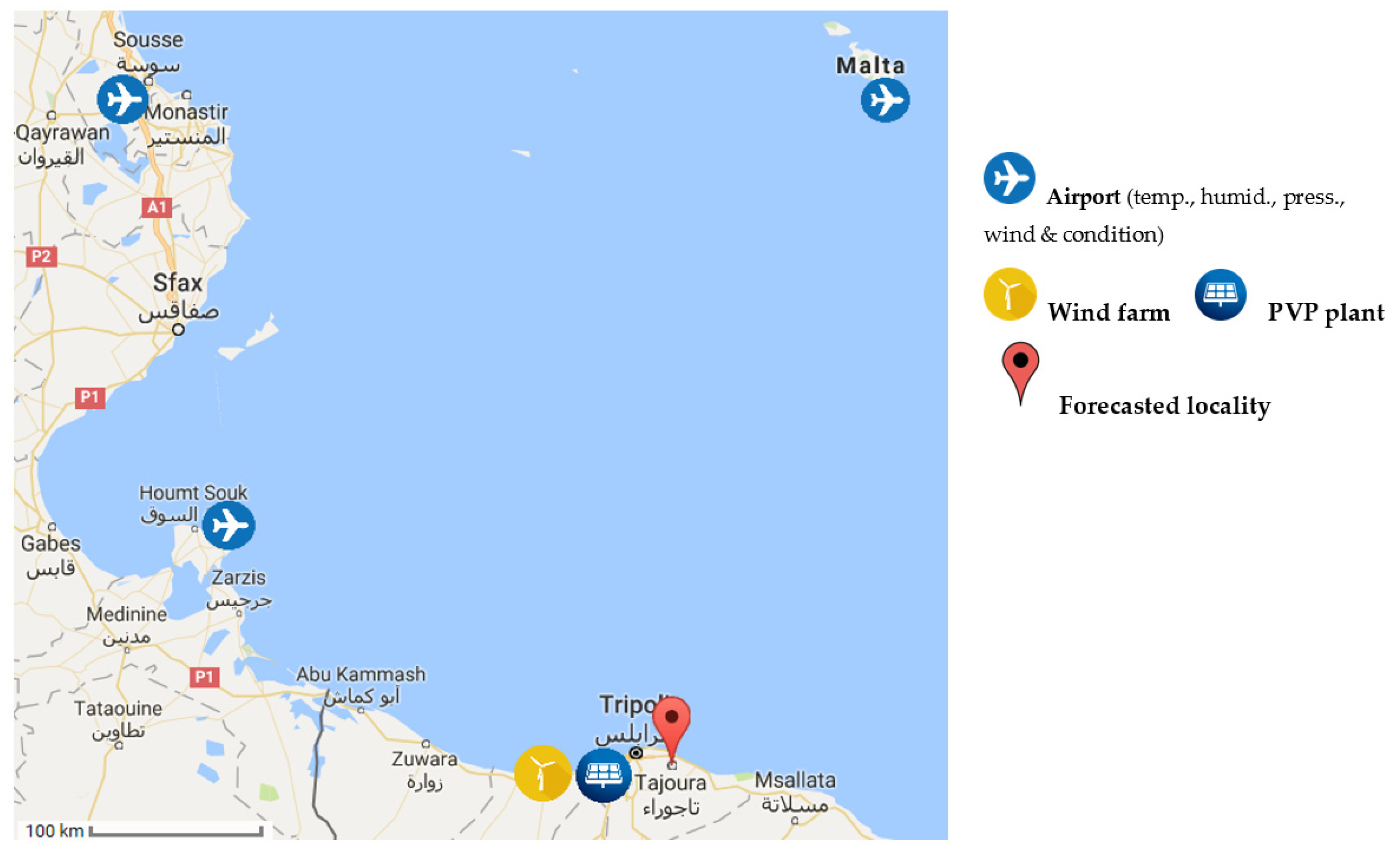
3. Observation Data and Methodology in Solar–Wind Series Mid-Term Forecasting

The initialisation time series intervals were redefined using the Pearson correlation distance (PCD), which most commonly expresses the measure of pattern similarity by determining strengths and directions in linear relationships in pairs of variables (1). The appropriate training samples were selected considering the PCD parameter [28]. The first initialisation time was searched for the best quantitative test output using a complementary simplified model. The day error minima were obtained for the gradually increasing day-to-day learning interval in the last 6 h test, indicating rough model initialisation [4]. The series contained in the first identified intervals were secondarily resampled by assessing pattern similarity at each time.

$$C{D}^{\prime }=1-CS=1-{\displaystyle \frac{\mathrm{cov}(P,Q)}{\sqrt{\mathrm{var}(P)}\cdot \sqrt{\mathrm{var}(Q)}}}=1-{\displaystyle \frac{{\displaystyle \sum _{k=1}^n\left(p_{ij}-\frac{1}{n}{\displaystyle \sum _{j=1}^n{p}_{ij}}\right)}\cdot {\displaystyle \sum _{k=1}^n\left(q_{ij}-\frac{1}{n}{\displaystyle \sum _{j=1}^n{q}_{ij}}\right)}}{\sqrt{{{\displaystyle \sum _{i=1}^n\left(p_{ij}-\frac{1}{n}{\displaystyle \sum _{j=1}^n{p}_{ij}}\right)}}^2}\cdot \sqrt{{{\displaystyle \sum _{i=1}^n\left(q_{ij}-\frac{1}{n}{\displaystyle \sum _{j=1}^n{q}_{ij}}\right)}}^2}}}$$

(1)

Figure 1 illustrates the starting search for fit day-sequence data by considering a single-time model initialisation in the step-by-step extended day interval of last hours validation. If initialisation models cannot obtain an adequate error threshold in relation to last-hour testing, the starting–end time days can be randomly shifted in testing. The best learning day bases can be identified by detecting breakover time changes in pattern re-analysis [7].

The prediction models were finally tested in the last observation hours to sequentially estimate 24 h solar/wind series in the processing of the last-day input [29]. Figure 2 presents the proposed day-ahead prediction strategy in developing self-optimising models. If an adequate test threshold cannot be reached, the statistical prognosis is flawed and should be accompanied by alternative NWP data. Capturing spatial border correlations of observational quantities in a midscale territory allows reliable validation of prediction models in the 24 h input–output horizon in a destination without NWP post-processing [7]. Pattern abnormalities or boundary non-stabilities in the last hours reflect unexpected dynamical changes in prediction times (storms, cyclones, or disturbing waves).

Figure 3 visualises the locations of ground-based airport stations with the target RE production facilities on the 100 km scale. Global radiation—horizontal (GR), direct radiation—normal (DNI), and horizontal radiation—diffuse (HD) were measured in 1 min recording series (2) at the Energy Research Centre [30] in Tajoura from 1 to 30 November 2015. Some data rows were not correctly recorded in the airport observational archives in Djerba and Monastir and had to be interpolated and replaced by averaging real data series at half-hour loss points [31]. The solar and wind speed (WS) data series were averaged to match the standard weather 30 min observational time and unify them with the reference recording at regional airports (compulsory meteo-monitoring). The station times of the airport observations in Luqa (+1 h) were shifted to relate them to the West Mediterranean time zone in Tajoura, Djerba, and Monastir [30,31].

GR = DNI + HD

(2)

GR = global radiation (horizontal), DNI = normal irradiance (direct), HD = diffuse radiation (horizontal) [W/m²].

4. Modelling Using AI Computational Tools

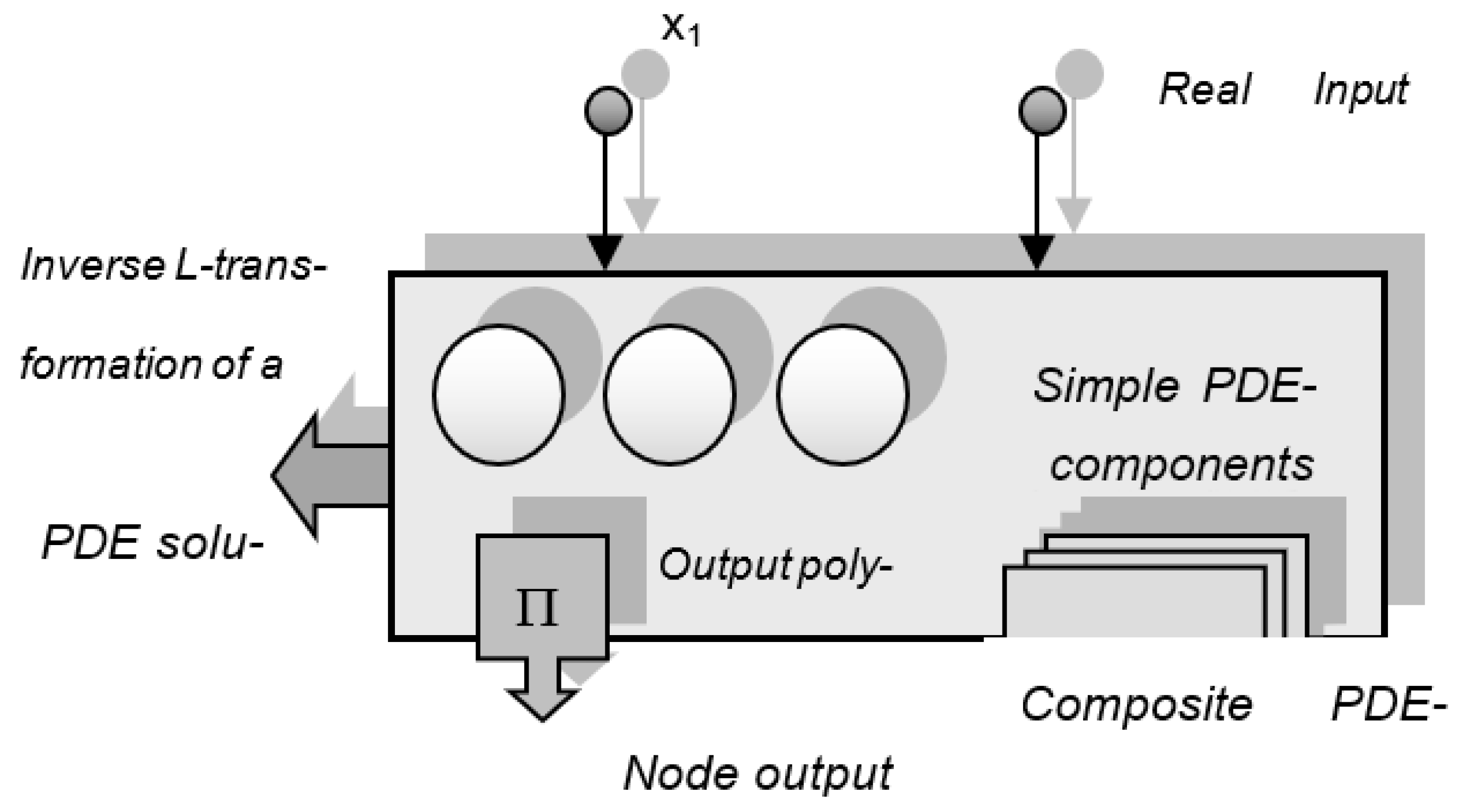
4.1. Differential Learning—An Innovative Neuro-Maths Computational Strategy

The differential polynomial neural network (D-PNN) is a recent atypical fused neuro-computing–maths regression tool, developed by the author. It combines machine learning principles based on non-linear artificial intelligence with mathematical procedures and definitions. The D-PNN parses the general linear type of a partial linear differential equation (PDE) to a simplified two-input PDE and converts transformed nodes of recognised orders (3). The D-PNN can model uncertain and chaotic dynamic systems whose behaviour is difficult to express by an exact mathematical definition. The evolution of the DBN model comprises efficient feature extraction that overcomes conventional regression and AI computing that requires additional pre-processing of data input. It gradually develops a multilayer binomial tree (BT), by extending its structure node by node into processed layers, to form and select applicable PDE modules in the BT nodes. The modules are tested and selected to be added to or extracted from the model sum to calculate and reach both training and testing error minima. Progressive model expansion using the PDE concept usually allows one to find the optimal solution to machine learning problems by employing Goedel’s incompleteness theorem. Each node in BT selects applicable variables, produced by nodes in back-connected layers, to determine sub-PDEs according to OC procedures. Its models can represent highly complex systems, described by dozens of data variables and hidden correlations. The order of binomials is related to the transformed PDE order [29].

$$A{\displaystyle \frac{{\partial }^{2}u}{\partial x_1^2}}+B{\displaystyle \frac{{\partial }^{2}u}{\partial x_1{x}_2}}+C{\displaystyle \frac{{\partial }^{2}u}{\partial x_2^2}}+D{\displaystyle \frac{\partial u}{\partial x_1}}+E{\displaystyle \frac{\partial u}{\partial x_2}}+Fu=G$$

(3)

A, B, …, G—param. coeff. for x₁, x₂ variables of the original u(x₁, x₂) function.

The polynomial transformation of f(t) is based on an OC definition for the L-transform (Laplace t.) of the nth PDE derivative in relation to the initial states (4).

$$L\left\{f^{(n)}(t)\right\}=p^{n}F(p)-{\displaystyle \sum _{k=1}^n{p}^{n-i}{f}_{0+}^{(i-1)}}\hspace{1em}\hspace{1em}L\left\{f(t)\right\}=F(p)$$

(4)

f(t), f’(t), …, f⁽ⁿ⁾(t)—contin. originals in <0+, ∞>. F(p)—complex form of the original f(t), p & t—complex & real variables in L{} transform.

The derivations of f(t) are OC converted to mathematical form (4), where the L images F(p) are separated into complex variables p in a ratio expression (5).

$$F(p)={\displaystyle \frac{P(p)}{Q(p)}}={\displaystyle \frac{Bp+C}{p^2+ap+b}}={\displaystyle \sum _{k=1}^n\frac{A_k}{p-{\alpha }_k}}$$

(5)

B, C, A_k—fractional elementary coeff. a, b—polynom.coeff.of α₁, α₂, …, α_k roots (real) of Q(p).

The pure F(p) ratios (5) correspond to the transform function f(t), which requires inverse recovery using the OC expressions (6) to calculate f(t) in the original non-imagery form by solving the defined ordinary differential equation (ODE) in this way [32].

$$F(p)={\displaystyle \frac{P(p)}{Q(p)}}={\displaystyle \sum _{k=1}^n\frac{P({\alpha }_k)}{Q_k({\alpha }_k)}}\cdot {\displaystyle \frac{1}{p-{\alpha }_k}}\hspace{1em}\hspace{1em}\hspace{1em}f(t)={\displaystyle \sum _{k=1}^n\frac{P({\alpha }_k)}{Q_k({\alpha }_k)}}{e}^{{\alpha }_k\cdot t}$$

(6)

P(p), Q(p)—s-1, s degree continuous polynom. Form α₁, α₂, …, α_n—Q(p) roots(real). p—complex var.

If f(t) is expressed in a periodic ODE type, the derivative is transformed into sine–cosine conversions, assuming the originals are recovering inversely in the same way (7). This extension formula for the frequency/amplitude data is used to compute the L-images of unknown node function origins.

$$f(t)={\displaystyle \sum _{k=1}^r\frac{P({\alpha }_k)}{Q^{\prime }({\alpha }_k)}}{e}^{{\alpha }_k\cdot t}+2{\displaystyle \sum _{k=1}^s{e}^{{\beta }_k\cdot t}}(a_k\cdot \cos {\gamma }_{k}t-b_k\cdot \sin {\gamma }_{k}t)$$

(7)

γ_k—complex conjugate roots of Q(p). t—time variable

The reverse L operation is applied to the periodic or ratio form (6), (7) of the transform functions, using the node definition (9), (10). The restored original functions u_k produced in the BT nodes (Figure 4) are summed to give the separable output u (3).

The Euler definition for a complex expressed c (8) represented in polar coordinates is related to OC (6). The parameter r is the radius (the part of the amplitude), related to the term of the ratio and the angle (that is, the part of the phase) ϕ = arctg(x₂/x₁), where the real nodes x₁, x₂ determine the reverse L-restoration of F(p) (5) [32].

$$c=\underset{\mathrm{Re}}{\underbrace{x_1}}+i\cdot \underset{\mathrm{Im}}{\underbrace{x_2}}=\sqrt{x_1^2+x_2^2}\cdot e^{i\cdot \arctan \left({\displaystyle \frac{x_2}{x_1}}\right)}=r\cdot e^{i\cdot \varphi }=r\cdot (\cos \varphi +i\cdot \sin \varphi )$$

(8)

ϕ—phase angle, r—amplit., i—imaginary conjugate, c—Euler’s complex representation.

Possible rational and periodic real-valued PDE transformations for the selected BT node input x₁, x₂ based on the adapted ODE definitions (6), (7) of OC with the final inverse recovery of the original output y using the exponential function are shown in Equations (9) and (10).

$${\mathrm{y}}_{\mathrm{j}}={\mathrm{w}}_{\mathrm{j}}{\displaystyle \frac{{\mathrm{b}}_0+{\mathrm{b}}_1{\mathrm{x}}_1+{\mathrm{b}}_2{\mathrm{x}}_2+{\mathrm{b}}_3{\mathrm{x}}_1{\mathrm{x}}_2}{{\mathrm{a}}_0+{\mathrm{a}}_1{\mathrm{x}}_1+{\mathrm{a}}_2{\mathrm{x}}_2+{\mathrm{a}}_3{\mathrm{x}}_1{\mathrm{x}}_2+{\mathrm{a}}_4\mathrm{sig}\left({\mathrm{x}}_1^2\right)+{\mathrm{a}}_5\mathrm{sig}\left({\mathrm{x}}_2^2\right)}}\cdot {\mathrm{e}}^{\mathrm{\phi }}$$

(9)

y_j—rational sub-PDE terms for u_k sum in nodes, sig—sigmoidal transform (optional); φ = arctg(x₂/x₁)—phase of two-input variables x₁, x₂. a_i, b_i, w_j—polynomial parameters and term weights.

y_i = [a₁ × ₁.cos(b₁2π.γ₁.t + b₀) − a₂x₂.sin(b₂2π.γ₂.t + b₀)] × e^ϕ

(10)

y_i—periodic output of node PDE-terms. γ₁, γ₂—phases [radian]. x₁, x₂—real amplitudes, a, b—coeff.

The D-PNN incremental leading innovations are as follows [33]:

• Parsing the n-dimensional PDE into self-recognised PDE node transform solutions
• Progressive evolving trees, adding nodes, one by one, in a back-computing framework
• Automatic selection of single PDE modules in nodes to extend the summary model
• Diverse types of PDE conversion functions using adapted OC in the model composition
• Derivative L-converted PDE and the OC inverse operation to obtain the node originals
• Recognition of the input optima in evolving tree structures producing PDE components
• Input dimensionality is not over-reduced, which prevents model simplification
• Combinatorial PDE node modular solutions in optimal pattern representation

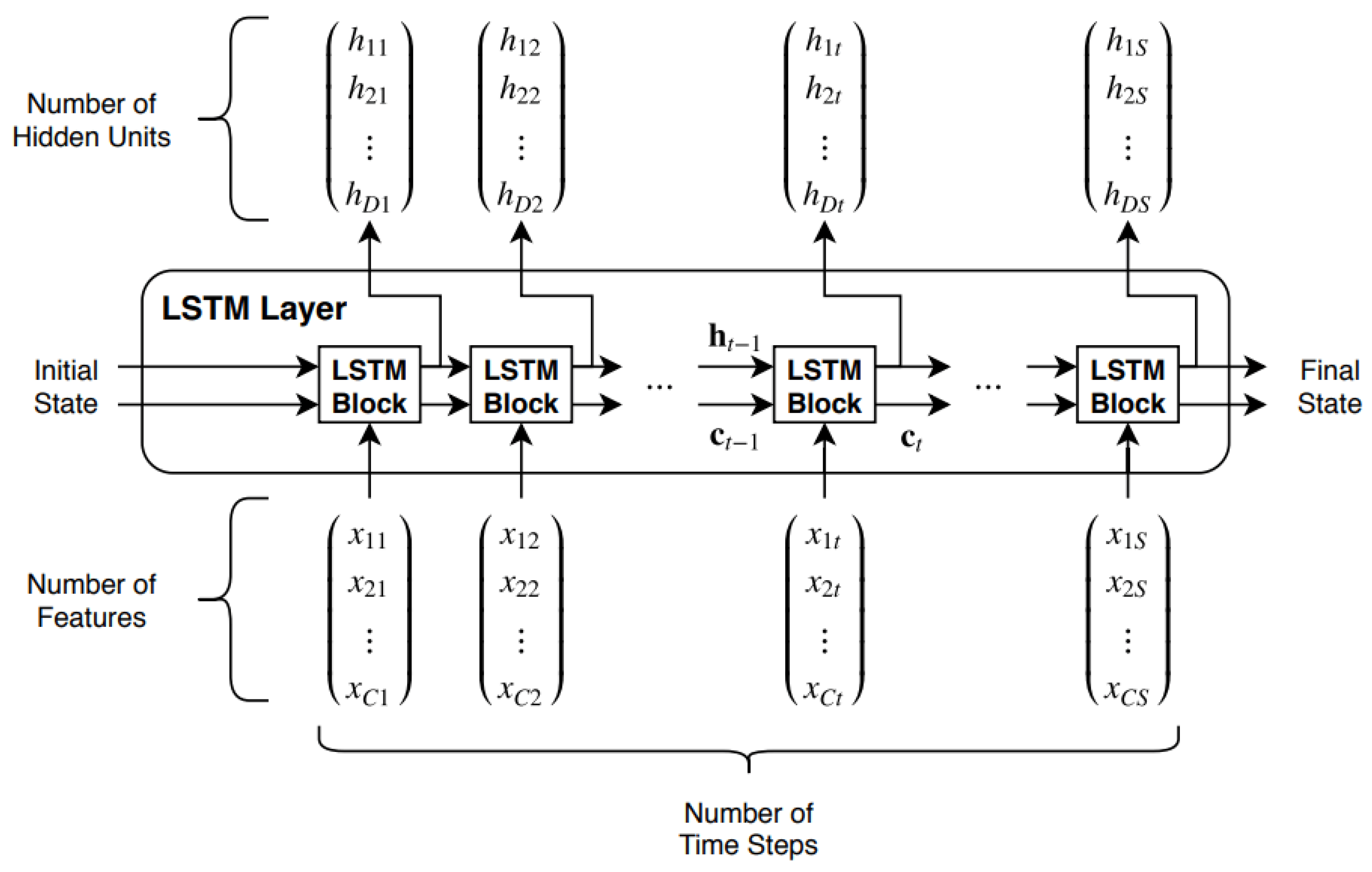
4.2. Matlab—LSTM Deep Learning

The Matlab Deep Learning Toolbox (DLT) is a sequence-to-sequence regression tool that employs an architecture based on long-short-term memory (LSTM). The two key layers of this neurocomputing approach are input sequenced and LSTM layers; the framework consists of the following:

• First layer: Sequence input
• Second layer: LSTM network
• Third layer: Fully connecting
• Fourth layer: Dropout
• Fifth layer: Fully connecting (regress)
• Sixth layer: Output net regression

The sequenced layer is entered by input sequenced series to feed the main layer LSTM, which is trained to long-term correlations of sequenced data in successive times. Its LSTM blocks process the states (c_t−1, h_t−1) and the next X sequences in time t to compute the output hidden state ht, updating the cell states c_t at times t (Figure 5). The state of cells comprises trained information from previous time steps by updating the information in the layer. The states in the layer are assessed as the hidden one h_t (i.e., the target output) associated with the states of the cells c_t. The dropout layer zero-sets the inputs in a randomised approach according to the defined (recognised) probability, which prevents network overfitting. A loss function is computed as a gradient using the set batch size in subsets of training data with changes in parameters and weights [30].

DLT architectures fuse multisequence data processing, based on forward- and backpropagation operation and computing principles of neural nets, with memory cell-weighted gates restoring long-term time dependencies. DLT uses an embedded LSTM layer to capture relevant pattern representations from input/output data in training. The DLT framework includes an experimental architecture design and setting using replicate structures that involve convolution, dropout, or other types of hidden layer blocks [32].

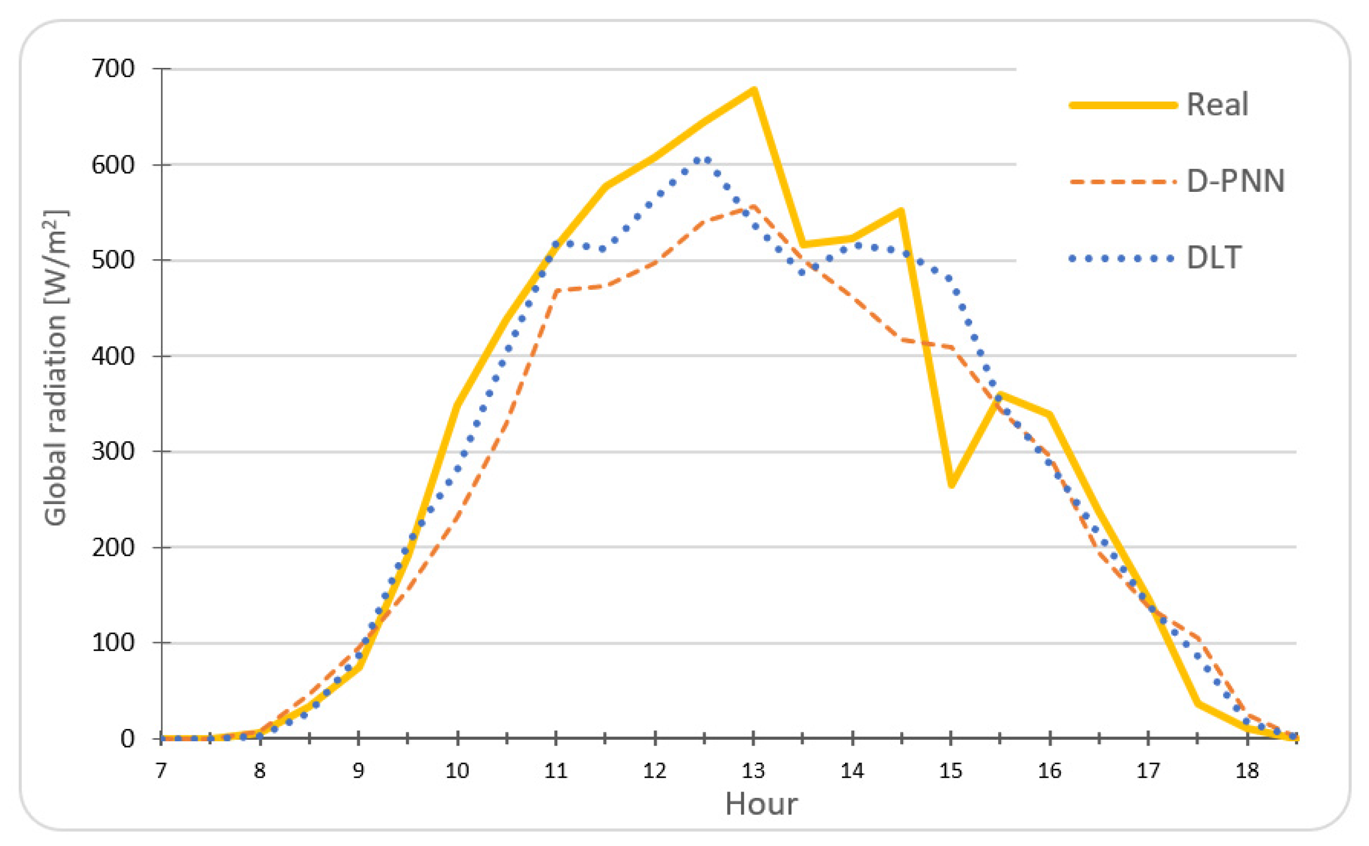
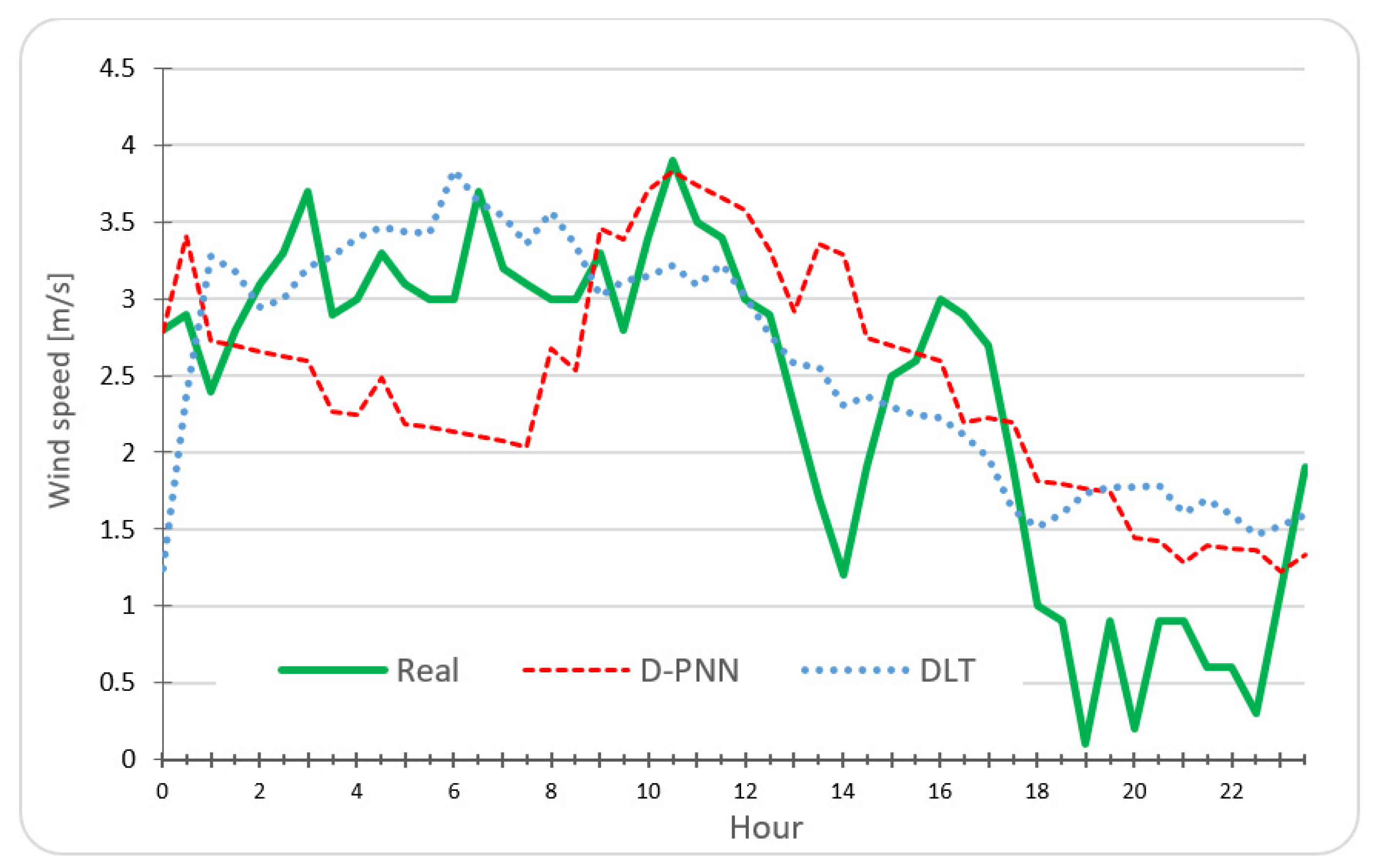
5. Day-Ahead Solar/Wind Statistical Predictions—Data Experiments

The desired real and computed series of GR between 7–19 h and WS in all 24 h on a common trouble-free prediction day are demonstrated by the graphs of Figure 6 and Figure 7, in comparison with the modular DfL and LSTM-based DLT models in the 10-day experimental autumn period. The pattern characteristics in the subsequent day interval remain like those of the day-illustrative graph. On 21 November an overnight break in changeable weather is recorded, and the next prediction days (Figure 1 and Figure 2) become sunny and gusty [30].

Both modelling approaches mostly correctly estimate the progress of target outputs in various ramping events of day cycles with less meaningful pattern over-changes. Their results outperform those obtained by the MATLAB Statistics and Machine Learning Toolbox [34]. The solar series were normalised to clear sky index (CSI) data, eliminating the day–time periodical character in noon maximum that refers to the current solar sky position. Standardised periodical data were expressed in the ratio of ideal ‘clear sky’ sequence maxima, to allow the processing and computation of the series regardless of the current day cycle time or season. The GR output is renormalised from the CSI standard in prediction [2]. Cycle quantities are generally correlated with the day amplitude time, applied in the periodic conversion of PDEs (7) to the node components of D-PNN. Periodical inputs such as GR, DNI, ground temperature and humidity, or wind azimuth variables were automatically recognised and processed in the DfL development of modular models.

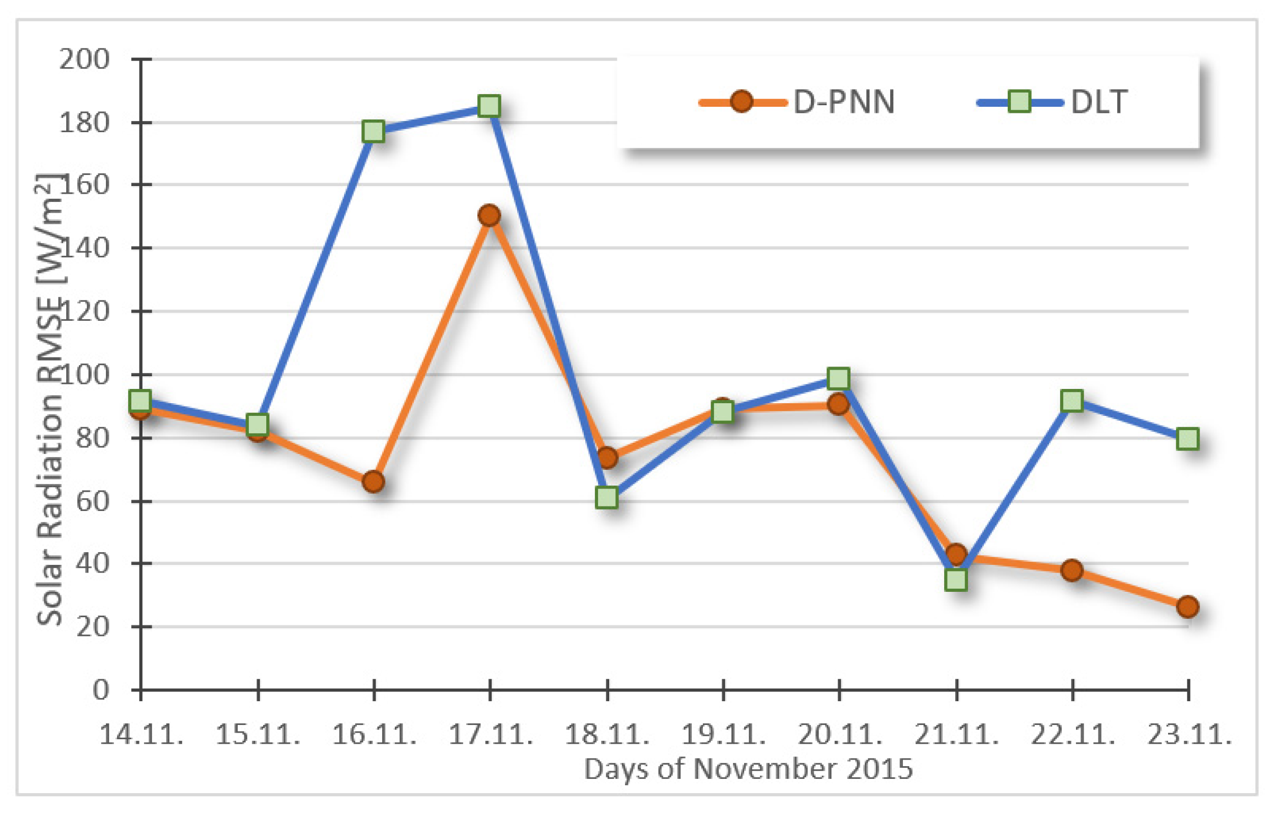
6. Day-Ahead Statistical Estimations of Solar/Wind Experiment Evaluation

Figure 8 and Figure 9 show the day aver. predictive errors of WS and GR in the 10-day evaluation period comparing both types of neurocomputing models, processing half-hour input series in all next-day sequential periods.

The variability in wind patterns on 15 and 20 November (Figure 2) results in a partial loss of statistical modelling quality (Figure 9). Sources of bias error could be found and eliminated by analytical methods on large archive data in training optimisation (1). A drop in the solar peak on 16 November (Figure 1) causes difficulties in AI-based learning for the next-day prediction (Figure 8). The applicability of statistics is mainly determined by the appropriate day initialisation time obtained at the start-model assessment. Figure 10 and Figure 11 show the PCD of the DfL and DLT estimates in the 24 h GR and WS series based on the previous 24 h sequential input processing in the 10-day experiments. Both neuro-based strategies, using only observational training data, produce similar prediction outputs that slightly differ in GR, although DfL considerably outperforms DLT in prediction WS. The low PCD values of DLT (slightly above zero) indicate an undesired WS output averaging and problems in the acceptable approximation of WS ramps. These inadequacies may be the consequence of unforeseen gust irregularities and the resulting computing uncertainty [2].

Both ML-modelling techniques obtained a moderate increase in PCD in the consequent approximation of regular GR day cycles (Figure 10). Short ramping events in WS gusts evidently result in larger alteration in PCD and troubles in consistency and adaptation of DLT models in some prediction times as compared to DfL (Figure 11).

The reliability in GR and WS prediction is mainly determined by the consistent day-training intervals, detected in initialisation day series for input–output time shifts. The selection of data samples is based on defined similarity measures in the n-dimensional input space (1) [28]. Forecasting and training patterns generally differ in degree of similarity (predictability) depending on over-changes in the atmosphere. Statistical models mostly do not allow for covering all eventual strong breaks in the atmosphere. Chaotic anomalies in weather patterns (Figure 7) can result in unexpected short-term events that are difficult to capture and substantially imply the approximation ability of ML models.

Figure 12 and Figure 13 show the day aver. error biases in the GR/WS prediction. The graphs give only informative insight, as the data in the 10-day evaluation period do not allow for a deeper analysis and interpretation of results to generalise model performance. The biases of both compared ML techniques (based on different computing principles) are noticeably correlated, which implies a strong impact of data pattern progress on predictability. The D-PNN produces slightly more stable bias output, without notable alterations. The bias of the DLT models is lower possibly due to the straight–gradient optimisation (in fixed–flat architecture), which is more complex in dynamical DfL structural development (using several selection and adaptation algorithms) and not fully solved yet. The first assessed initialisation day–time periods were used in computing optimal pattern similarity distances to reveal optimal-correlation input–output samples (Figure 14 and Figure 15).

The quality of ML predictions is primarily determined by the dynamical variability in patterns and adequately represented data relations within the applied input–output time shift. Secondary data resampling based on a kind of correlation statistics helps to reduce the unambiguity in unexpected over-breaks. DfL and DL are able to forecast in a day horizon using a sophisticated sample selection on available data if they allow the capturing of regular all-over day-pattern changes (Figure 12 and Figure 13). The main limitation of AI-based forecasting lies in the accessibility to large historical observations, and NWP repositories searched for similar pattern progress and the interpretation of model failures in correcting training. Comparative data evaluation for analogous case situations will help to compete with large NWP systems able to simulate the atmosphere behaviour in several coming days according to physical laws, despite their high computational demands. AI-based post-processing utilities that employ the proposed statistics can accommodate NWP output by eliminating possible local inadequacies in forecasting.

7. Discussion

The designed DfL evolves neurotransform models in selective binary tree-like structures at each node evaluation step. The inputs and node-produced PDE components are progressively reselected, inserted, or reduced in each iteration to be included in the model, starting empty. The first added and redundant PDE components are continually re-evaluated in each model update to maintain the essential binomial connections in optimal node compositions. The architecture and model form are not initially manually designed, as usual in DL, but are gradually self-evolved and determined in training. The secondary applied phase input (e.g., wind azimuth) used in the periodic PDE node conversion improves the representation of cycle characteristics. Different node PDE substitutions contribute to optimal combinatorial solutions in capturing pattern dynamics. Their diversity and modularity improve the processing of unseen input in an uncertain environment, which are the main benefits compared to conventional fixed-layer neurocomputing. No reduction in data dimensionality is necessary in the first processing, leading to eventual parametric and structural degradation in model representation, common in soft computing. The time costs and complexity in model self-evolution are naturally higher as compared to the traditional DL experimental design; however, the DfL versatility in model definition and readapt ability prevails over the optimisation expenses. The key implications are as follows: searching large data archives for similar pattern progress in extended training sets helps better recognise specific cases necessary in optimal ML model adaptation to the current atmospheric trend over prediction time. AI promptness in proper detection and learning up-to-date relations from big data, representing forthcoming situation progress by improving its skills step by step, is the major advantage as compared to alternative NWP simulations.

Time-assessed models in reduced horizons can refine the day-ahead first estimates by the re-optimised initialisation. The ML statistical output is naturally advisable to compare with a physical NWP, if available in time. In doubtful multivalent solutions of several NWP or AI models, the results are interpreted according to their current performance in a selected time window to choose the most reliable forecast in RE utilisation. Local atmospheric events usually result from complex ground interactions in the adjacent layer, terrain obstacle disturbances in air flow, or instabilities. These ambiguous irregularities can cause the inapplicability of observational data in evolutionary AI modelling statistics in the predefined 24 h mid-term horizon. The first initial detection of training samples can be reassigned in more complex pre-processing based on characteristics in historical patterns and the latest error re-analysis. Defined comparative thresholds between NWP and observational data can help avoid statistical model flaws in predictive times. Critical modelling failures can be re-evaluated considering rapid changes in pattern progress to detect bias and parametric sources. Large databases can be used to detect adequate intervals in model initialisation time (Figure 10). A detailed interpretation of prediction errors in relation to the characteristics of test patterns [31] can be used to approve the results in disputable cases with inconsistent model performance [20]. Extension with 24 h cycle delay input improves statistical model stability in objectionable prediction times (e.g., humidity and temperature, solar and PVP series).

The aimed incremental training keeps the previously learnt data knowledge of the original model. The proposed modular DfL gradually refines and extends the optimal model form by reducing useless/incorporating new PDE components. New data samples are to be used in additional training in re-evolving previous structures and the related node-produced PDE subsolutions. The model could be systematically adjusted day by day to new input–output patterns to be more compact and eligible for unexpected changes in each next predictive computing session.

8. Conclusions

The sequenced prediction procedure using all-day optimising models evidently simplifies and accelerates 24 h computing. Reduced modelling time costs are notable in comparison to separately evolved models in each prediction time or NWP simulation delay. The benefits arise from the generalisation of one self-adapted model in a fixed training-assessed input–output time shift in day-ahead estimation. The main motivation is innovative pre-processing that improves ML predictability using a type of similarity sampling by re-evaluating training intervals to reveal characteristic data patterns. The procedure was tested and experimentally approved in the GR and WS case models. Optimal feature selection and detection of training samples based on sophisticated model initialisation are crucial for all recently introduced hybrid methodologies. The better approximation ability of DfL results from the flexibility of node-by-node dynamically composed trees in producing multivariate PDE solutions that properly reflect long/short-time events, compared to conventional frameworks. Future research will incorporate the periodic node PDE transformation into a doubled complex form. The daily percentage forecast accuracy obtained on average RMSE and PCD in GR corresponds to those shown in the literature, reaching slightly below 90%. Predictive results in WS are limited by monthly data available in learning, where rapid fluctuations are not adequately related to data variability under a longer time horizon in specific daily changeable conditions. Spatial archive data improve ML predictability in mid-term horizons in modelling boundary conditions crucial in representing pattern progress in a target location.

Early support that provides first-forward NWP conversions of GR and WS is useful in preparing raw RE production plans. Operational strategies generally require daily forecasts of adequate quality and validity. Sophisticated intraday local hourly predictions based on AI analytics usually obtain better precision than regional NWP. Numerical systems are naturally good at recognising breaking changes in weather day progress, where AI training based on modelling historical patterns may fail, especially if larger data archives are missing. The unstable hourly output of statistical models denotes an inadequate pattern representation under future conditions. AI prediction could be confirmed by NWP utilities or re-analysing daily operational planning in these casual situations.

References

1. Onteru, R.R.; Sandeep, V. An intelligent model for efficient load forecasting and sustainable energy management in sustainable microgrids. Discov. Sustain. 2024, 5, 170. [Google Scholar] [CrossRef]
2. Zjavka, L. Wind speed and global radiation forecasting based on differential, deep and stochastic machine learning of patterns in 2-level historical meteo-quantity sets. Complex Intell. Syst. 2023, 9, 3871–3885. [Google Scholar] [CrossRef]
3. Zhang, G.; Yang, D.; Galanis, G.; Androulakis, E. Solar forecasting with hourly updated numerical weather prediction. Renew. Sustain. Energy Rev. 2024, 154, 111768. [Google Scholar] [CrossRef]
4. Zjavka, L. Power quality validation in micro off-grid daily load using modular differential, lstm deep, and probability statistics models processing nwp-data. Syst. Sci. Control Eng. 2024, 12, 2395400. [Google Scholar] [CrossRef]
5. Verbois, A.T.H.; Saint-Drenan, Y.-M.; Blanc, P. Statistical learning for nwp post-processing: A benchmark for solar irradiance forecasting. Sol. Energy 2025, 235, 132–149. [Google Scholar] [CrossRef]
6. Zjavka, L.; Sokol, Z. Local improvements in numerical forecasts of relative humidity using polynomial solutions of general differential equations. Q. J. R. Meteorol. Soc. 2018, 144, 780–791. [Google Scholar] [CrossRef]
7. Zjavka, L. Photo-voltaic power intra-day and daily statistical predictions using sum models composed from l-transformed pde components in nodes of step by step developed polynomial neural networks. Electr. Eng. 2021, 103, 1183–1197. [Google Scholar] [CrossRef]
8. Blaga, R.; Sabadus, A.; Stefu, N.; Dughir, C. A current perspective on the accuracy of incoming solar energy forecasting. Prog. Energy Combust. Sci. 2019, 70, 119–144. [Google Scholar] [CrossRef]
9. Mulashani, A.K.; Shen, C.; Kawamala, M. Enhanced group method of data handling (gmdh) for permeability prediction based on the modified levenberg marquardt technique from well log data. Energy 2022, 239, 121915. [Google Scholar] [CrossRef]
10. Wang, Z.; Huang, H. Second-order structure optimization of fully complex-valued neural networks. IEEE Trans. Emerg. Top. Comput. Intell. 2024, 8, 2349–2363. [Google Scholar] [CrossRef]
11. Ahmed, R.; Sreeram, V.; Mishra, Y.; Arif, M.D. A review and evaluation of the state-of-the-art in pv solar power forecasting: Techniques and optimization. Renew. Sustain. Energy Rev. 2020, 124, 109792. [Google Scholar] [CrossRef]
12. Ahmad, H.A.; Xiao, X.; Dong, D. Tuning data preprocessing techniques for improved wind speed prediction. Energy Rep. 2024, 11, 287–303. [Google Scholar] [CrossRef]
13. Guermoui, M.; Melgani, F.; Danilo, C. Multi-step ahead forecasting of daily global and direct solar radiation: A review and case study of ghardaia region. J. Clean. Prod. 2018, 201, 716–734. [Google Scholar] [CrossRef]
14. Sørensen, M.L.; Nystrup, P.; Bjerregård, M.B.; Møller, J.K.; Bacher, P.; Madsen, H. Recent developments in multivariate wind and solar power forecasting. Energy Environ. 2022, 13, e465. [Google Scholar] [CrossRef]
15. Yakoub, G.; Mathew, S.; Leal, J. Power production forecast for distributed wind energy systems using support vector regression. Energy Sci. Eng. 2022, 10, 4662–4673. [Google Scholar] [CrossRef]
16. Kumari, P.; Toshniwal, D. Deep learning models for solar irradiance forecasting: A comprehensive review. J. Clean. Prod. 2021, 318, 128566. [Google Scholar] [CrossRef]
17. Huang, H.-H.; Huang, Y.-H. Probabilistic forecasting of regional solar power incorporating weather pattern diversity. Energy Rep. 2024, 11, 1711–1722. [Google Scholar] [CrossRef]
18. Ding, J.W.; Chuang, M.J.; Tseng, J.S.; Hsieh, I.Y.L. Reanalysis and ground station data: Advanced data preprocessing in deep learning for wind power prediction. Appl. Energy 2024, 375, 124129. [Google Scholar] [CrossRef]
19. Lindberg, O.; Lingfors, D.; Arnqvist, J.; van Der Meer, D.; Munkhammar, J. Day-ahead probabilistic forecasting at a co-located wind and solar power park in sweden: Trading and forecast verification. Adv. Appl. Energy 2023, 9, 100120. [Google Scholar] [CrossRef]
20. Gupta, P.; Singh, R. Forecasting hourly day-ahead solar photovoltaic power generation by assembling a new adaptive multivariate data analysis with a long short-term memory network. Sustain. Energy Grids Netw. 2023, 35, 101133. [Google Scholar] [CrossRef]
21. Wu, Y.; Qian, C.; Huang, H. Enhanced Air Quality Prediction Using a Coupled DVMD Informer-CNN-LSTM Model Optimized with Dung Beetle Algorithm. Entropy 2024, 26, 534. [Google Scholar] [CrossRef] [PubMed]
22. Phan, Q.-T.; Wu, Y.-K.; Phan, Q.-D.; Lo, H.-Y. A novel forecasting model for solar power generation by a deep learning framework with data preprocessing and postprocessing. IEEE Trans. Ind. Appl. 2023, 59, 220–233. [Google Scholar] [CrossRef]
23. Javaid, A.; Sajid, M.; Uddin, E.; Waqas, A.; Ayaz, Y. Sustainable urban energy solutions: Forecasting energy production for hybrid solar-wind systems. Energy Convers. Manag. 2024, 302, 118120. [Google Scholar] [CrossRef]
24. Wang, Y.; Zou, R.; Liu, F.; Zhang, L.; Liu, Q. A review of wind speed and wind power forecasting with deep neural networks. Appl. Energy 2021, 304, 117766. [Google Scholar] [CrossRef]
25. Guermoui, M.; Melgani, F.; Gairaa, K.; Mekhalfi, M.L. A comprehensive review of hybrid models for solar radiation forecasting. J. Clean. Prod. 2020, 258, 120357. [Google Scholar] [CrossRef]
26. Chen, S.; Li, C.; Stull, R.; Li, M. Improved satellite-based intra-day solar forecasting with a chain of deep learning models. Energy Convers. Manag. 2024, 313, 118598. [Google Scholar] [CrossRef]
27. Konstantinou, T.; Hatziargyriou, N. Day-ahead parametric probabilistic forecasting of wind and solar power generation using bounded probability distributions and hybrid neural networks. IEEE Trans. Sustain. Energy 2023, 14, 2109–2120. [Google Scholar] [CrossRef]
28. Tamás, F.; Edelmann, M.D.; Székely, G.J. On relationships between the pearson and the distance correlation coefficients. Stat. Probab. Lett. 2024, 169, 108960. [Google Scholar]
29. Zjavka, L. Power quality estimations for unknown binary combinations of electrical appliances based on the step-by-step increasing model complexity. Cybern. Syst. 2024, 35, 1184–1204. [Google Scholar] [CrossRef]
30. The Centre for Solar Energy Research in Tajoura City, Libya. Available online: www.csers.ly/en (accessed on 8 July 2025).
31. Weather Underground Historical Data Series: Luqa, Malta Weather History|Weather Underground (wunderground.com). Available online: www.wunderground.com/history/daily/mt/luqa/LMML (accessed on 8 July 2025).
32. Zjavka, L. Power quality 24-hour prediction using differential, deep and statistics machine learning based on weather data in an off-grid. J. Frankl. Inst. 2023, 360, 13712–13736. [Google Scholar] [CrossRef]
33. D-PNN Application C++ Parametric Software Incl. Solar, Wind & Meteo Spatial-Data. Available online: https://nextcloud.vsb.cz/s/EFDJ7mRyxfHkjSc (accessed on 8 July 2025).
34. Matlab—Statistics and Machine Learning Tool-Box for Regression (SMLT). Available online: www.mathworks.com/help/stats/choose-regression-model-options.html (accessed on 8 July 2025).
Figure 1. Estimation of initialisation time in a post-processing evaluation of similarity patterns.
Atmosphere 16 00859 g001
Figure 2. Model development, testing and prediction in estimating solar and wind series.
Atmosphere 16 00859 g002
Figure 3. The solar and wind destination locality in Tajoura and supporting airport stations in the South Mediterranean region.
Atmosphere 16 00859 g003
Figure 4. The BT node forms model components to convert and inversely resolve the 2-variable sub-PDEs.
Atmosphere 16 00859 g004
Figure 5. The LSTM layer: time series X flow in C feature channels with S length.
Atmosphere 16 00859 g005
Figure 6. 18 November 2015, Tajoura City, GR prediction aver. RMSE: D-PNN = 73.50, DLT = 60.63 [W/m2].
Atmosphere 16 00859 g006
Figure 7. 18 November 2015, Tajoura City, WS prediction aver. RMSE: D-PNN = 0.809, DLT = 0.690 [m/s].
Atmosphere 16 00859 g007
Figure 8. 10-day solar aver. day prediction RMSE: D-PNN = 74.74, DLT = 99.04 [W/m2].
Atmosphere 16 00859 g008
Figure 9. 10-day wind aver. day prediction RMSE: D-PNN = 0.826, DLT = 0.925 [m/s].
Atmosphere 16 00859 g009
Figure 10. 10-day radiation aver. prediction day correl. Determination param.: D-PNN = 0.878, DLT = 0.881 [].
Atmosphere 16 00859 g010
Figure 11. 10-day wind aver. day prediction correl. Determination param.: D-PNN = 0.467, DLT = 0.363 [].
Atmosphere 16 00859 g011
Figure 12. 10-day radiation aver. day prediction error bias: D-PNN = 87.01, DLT = 40.89 [W/m2].
Atmosphere 16 00859 g012
Figure 13. 10-day wind aver. day prediction error bias: D-PNN = 1,460, DLT = 0.032 [W/m2].
Atmosphere 16 00859 g013
Figure 14. The intervals initially assigned for the day data subseries used in selection of the optimal data samples in the evolution of the solar radiation models.
Atmosphere 16 00859 g014
Figure 15. The intervals initially assigned for the day data subseries used in selection of the optimal data samples in the evolution of the wind speed models.
Atmosphere 16 00859 g015
Disclaimer/Publisher’s Note: The statements, opinions and data contained in all publications are solely those of the individual author(s) and contributor(s) and not of MDPI and/or the editor(s). MDPI and/or the editor(s) disclaim responsibility for any injury to people or property resulting from any ideas, methods, instructions or products referred to in the content.