

An Improved Interpolation Algorithm for Surface Meteorological Observations via Fuzzy Adaptive Optimisation Fusion
 ,
,  , ,
, ,
Abstract
1. Introduction
2. Methods
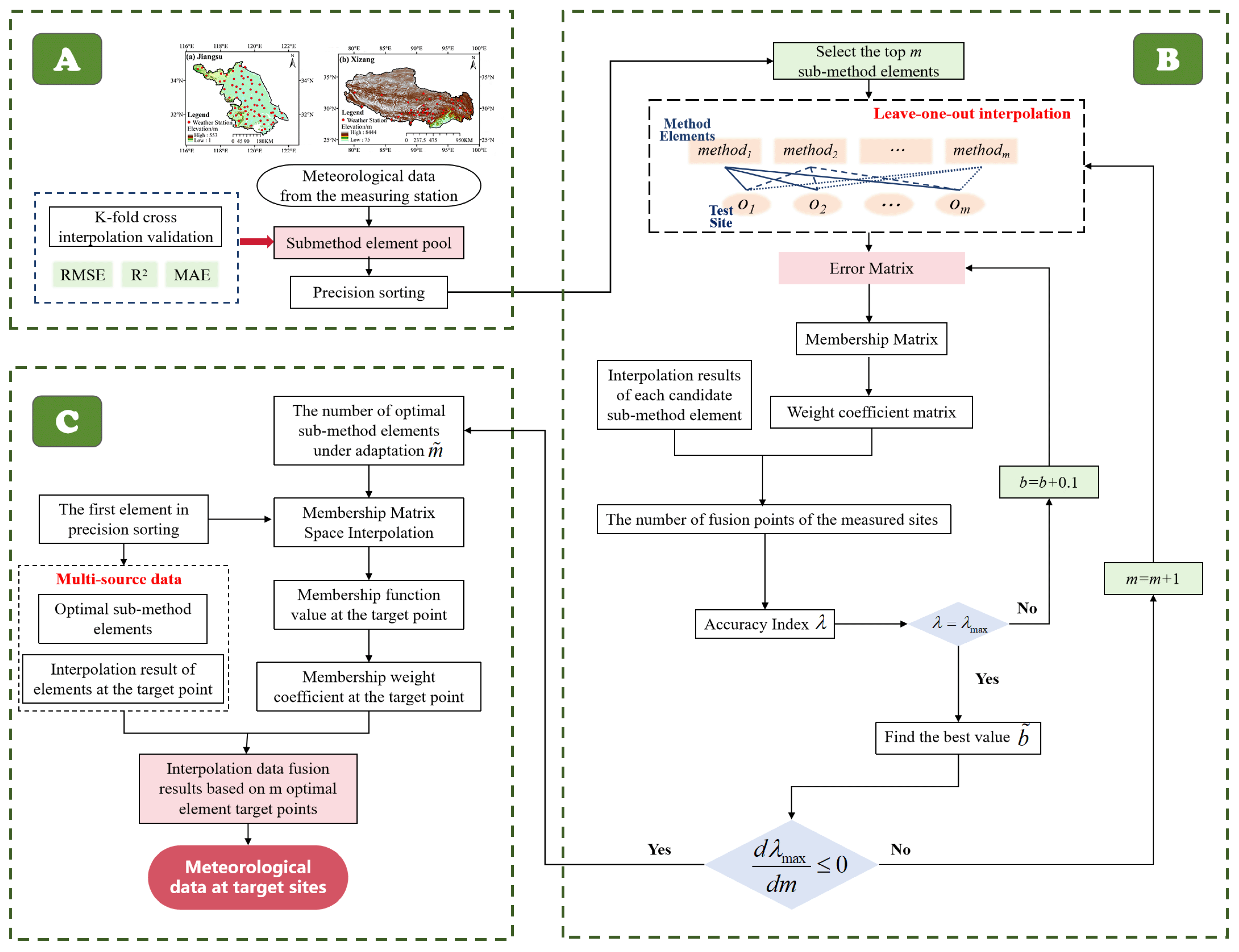
2.1. Fuzzy Theory
2.2. Sub-Method Element
2.3. Fuzzy Adaptive Optimisation Fusion Model
2.4. Performance Evaluation Indicators
3. Data
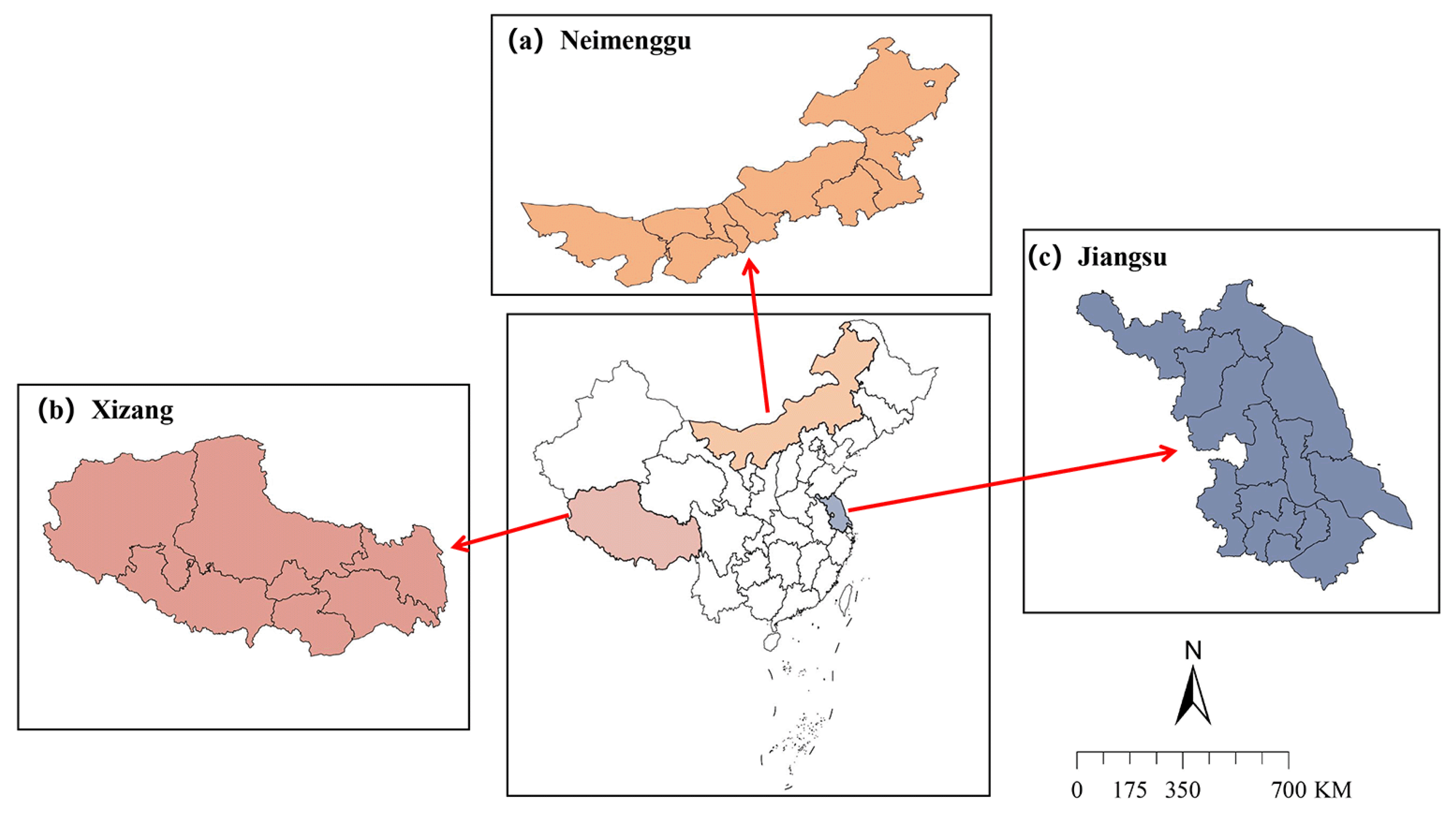
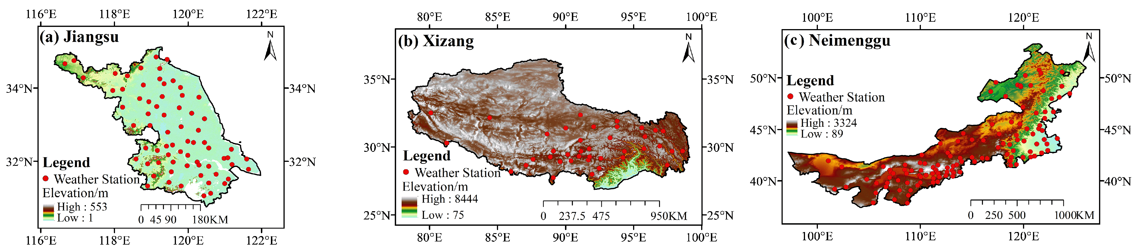
3.1. Study Area
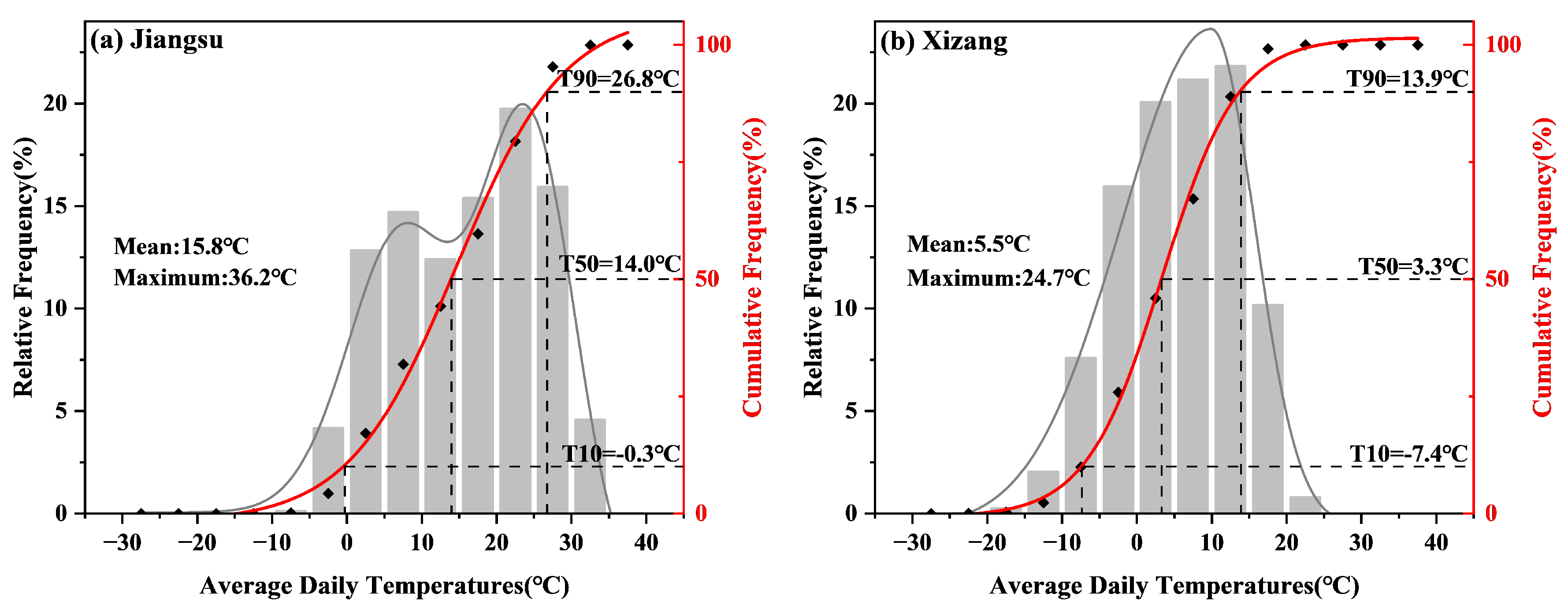
3.2. Dataset
4. Results and Discussion
4.1. Performance of the Interpolation Method for Surface Temperature
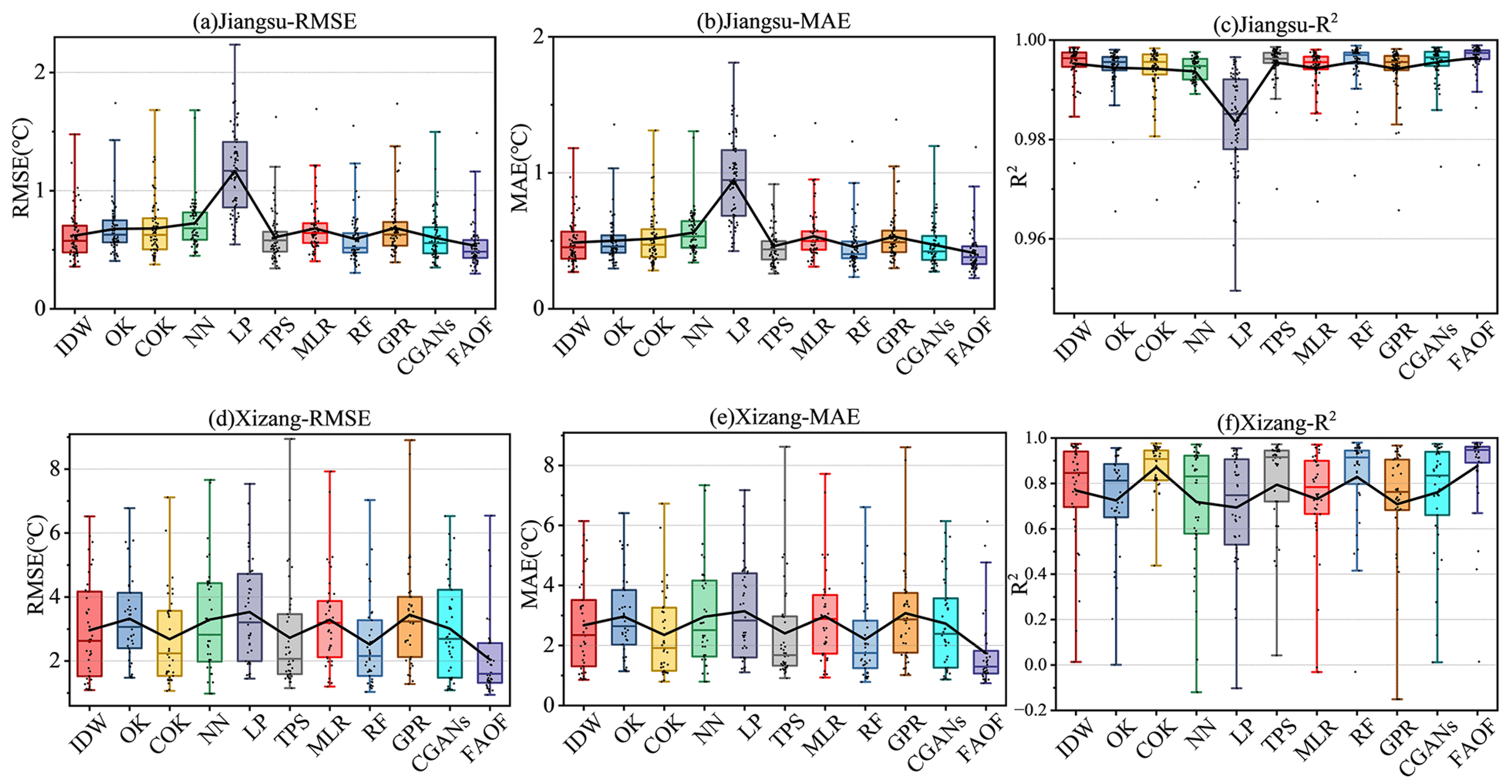
4.1.1. Analysis of the Overall Situation
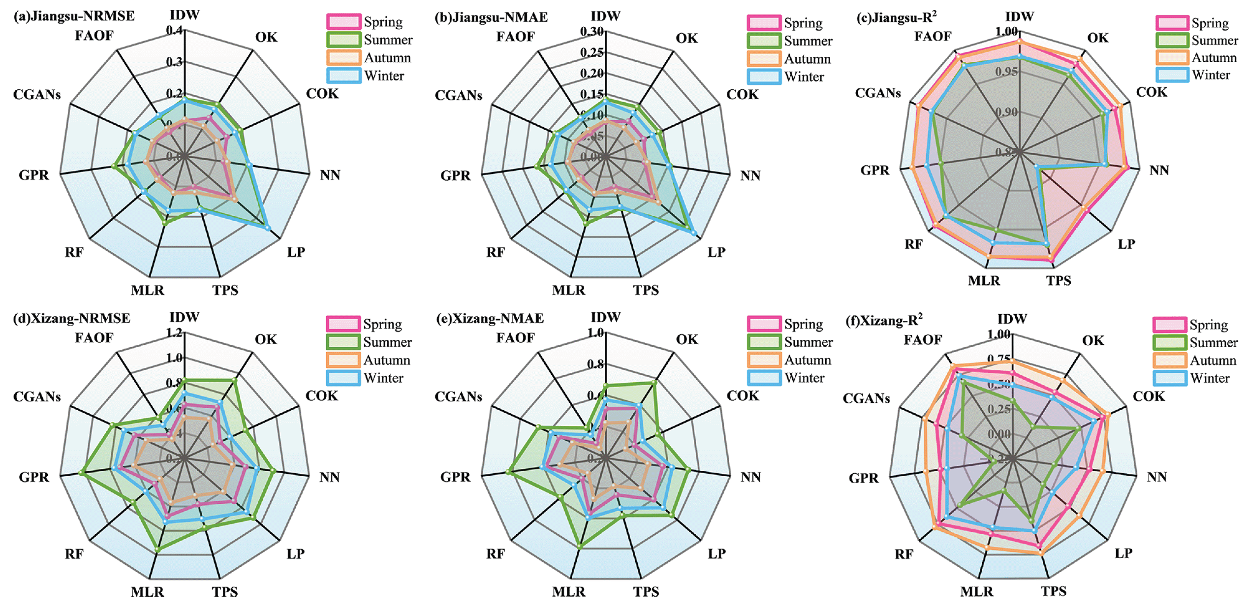
4.1.2. Performance in Different Seasons
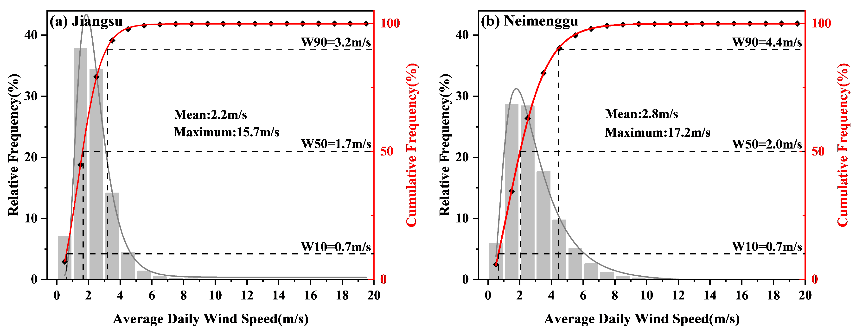
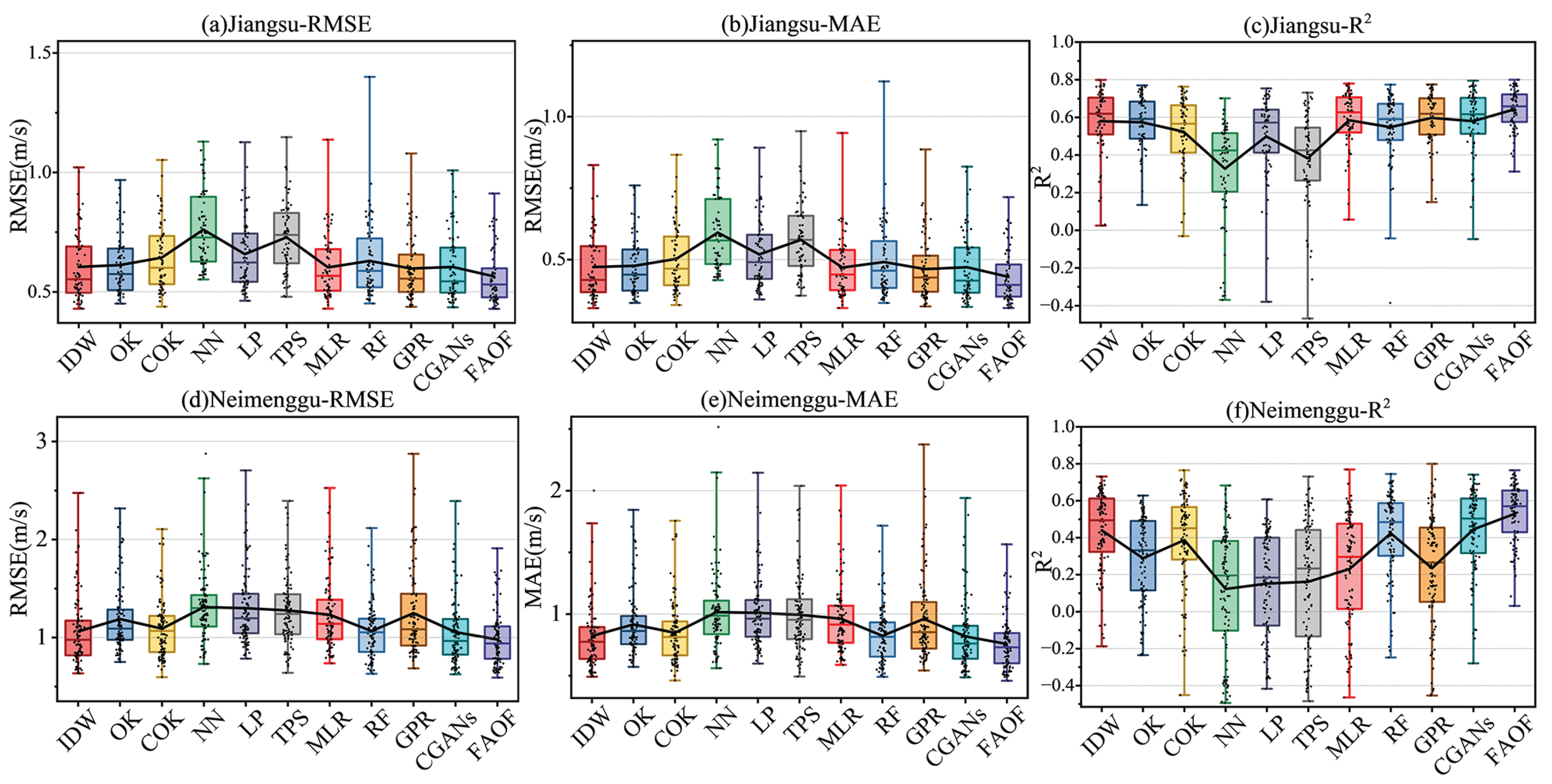
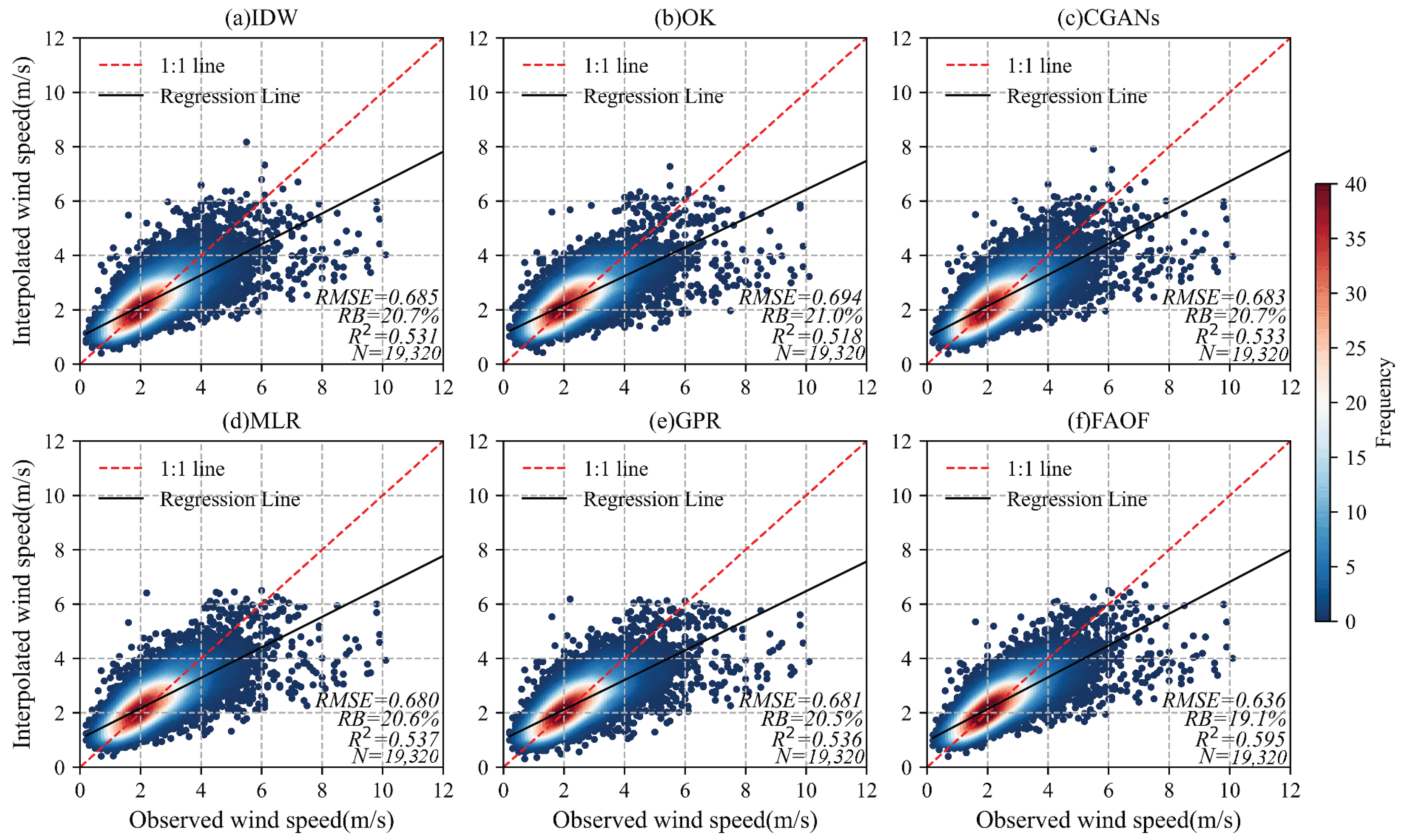
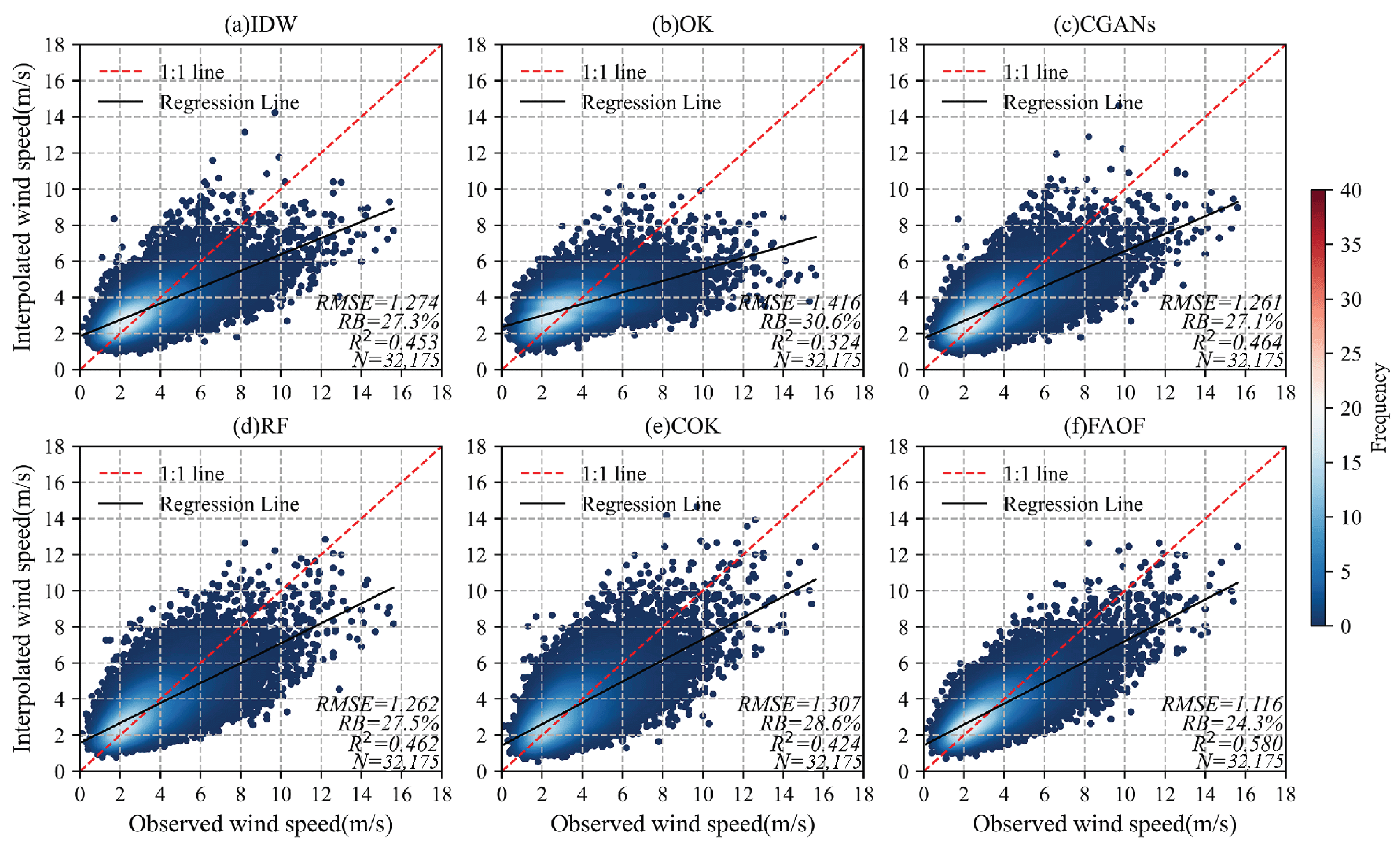
4.2. Performance of Wind Speed Interpolation
4.2.1. Analysis of the Overall Situation
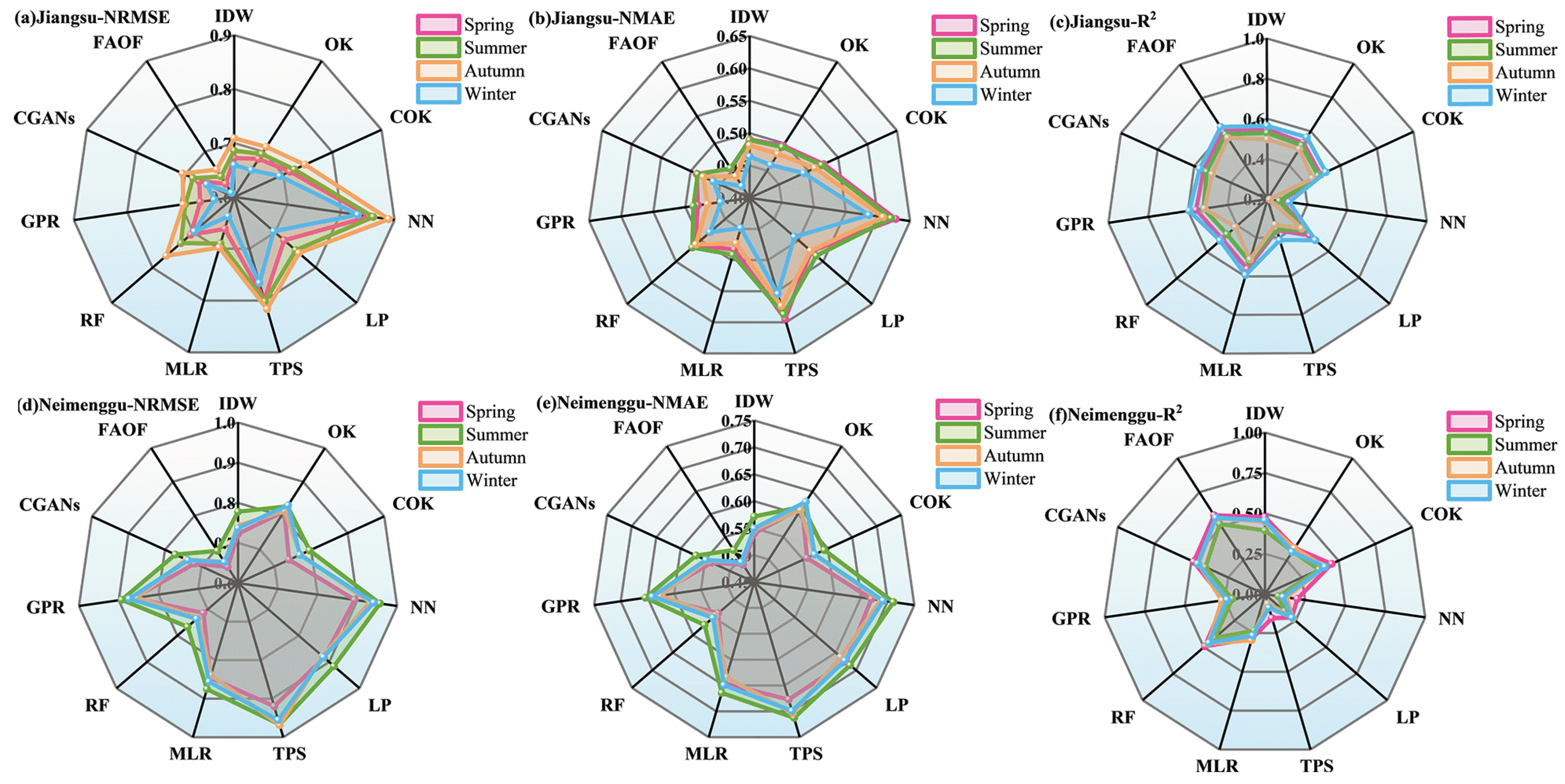
4.2.2. Performance in Different Seasons
5. Conclusions
- (1)
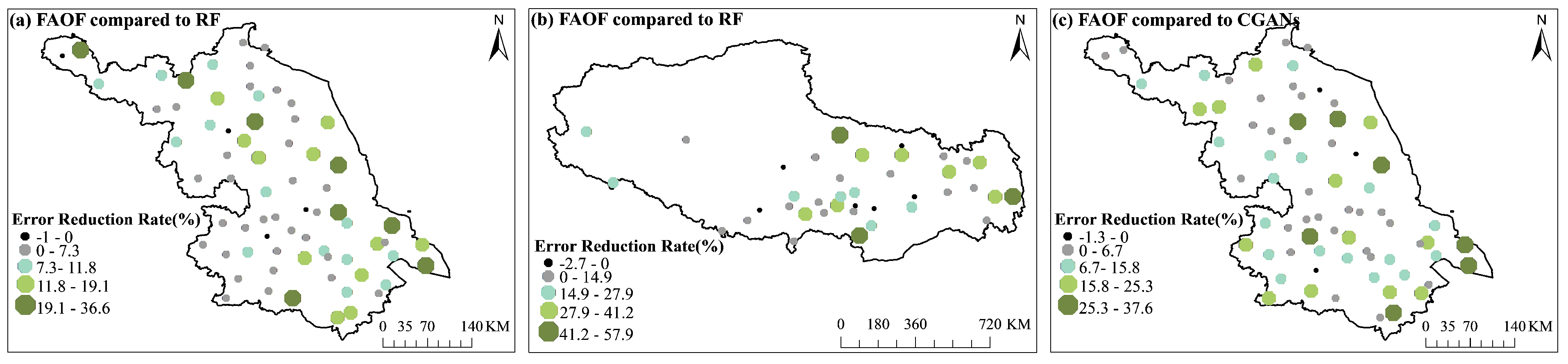
- Improved Accuracy: The FAOF method consistently outperforms the single-interpolation method for temperature and wind speed. It demonstrated high accuracy and consistency. This success is due to FAOF’s ability to reduce the limitations of individual methods while integrating their strengths.
- (2)
- Element-Specific Performance: All methods showed better goodness of fit for temperature, with R2 values closer to 1. This is attributed to the element’s continuity and smoothness. In contrast, wind speed exhibited lower coefficients of determination due to its fluctuating nature.
- (3)
- Adaptive Capabilities: The FAOF model demonstrated adaptability to diverse meteorological elements. This reflects the model’s flexible design and ability to optimise for varied data characteristics.
Author Contributions
Funding
Institutional Review Board Statement
Informed Consent Statement
Data Availability Statement
Acknowledgments
Conflicts of Interest
Abbreviations
| FAOF | Fuzzy Adaptive Optimal Fusion; |
| RMSE | Root Mean Square Error; |
| MAE | Mean Absolute Error; |
| RB | Relative Bias; |
| NRMSE | Normalised Root Mean Square Error; |
| NMAE | Normalised Mean Absolute Error; |
| IDW | Inverse Distance Weighting; |
| OK | Ordinary Kriging; |
| COK | Co-Kriging; |
| NN | Neural Network; |
| LP | Linear Programming; |
| TPS | Thin-Plate Spline; |
| MLR | Multiple Linear Regression; |
| RF | Random Forest; |
| GPR | Gaussian Process Regression; |
| CGANs | Conditional Generative Adversarial Networks. |
References
- Ye, P. Remote Sensing Approaches for Meteorological Disaster Monitoring: Recent Achievements and New Challenges. Int. J. Environ. Res. Public Health 2022, 19, 3701. [Google Scholar] [CrossRef] [PubMed]
- Delforge, D.; Wathelet, V.; Below, R.; Sofia, C.L.; Tonnelier, M.; van Loenhout, J.A.F.; Speybroeck, N. EM-DAT: The emergency events database. Int. J. Disaster Risk Reduct. 2023, 124, 105509. [Google Scholar] [CrossRef]
- Cao, S.; Zhang, L.; He, Y.; Zhang, Y.; Chen, Y.; Yao, S.; Yang, W.; Sun, Q. Effects and contributions of meteorological drought on agricultural drought under different climatic zones and vegetation types in Northwest China. Sci. Total Environ. 2022, 821, 153270. [Google Scholar] [CrossRef] [PubMed]
- Gilewski, P.; Nawalany, M. Inter-Comparison of Rain-Gauge, Radar, and Satellite (IMERG GPM) Precipitation Estimates Performance for Rainfall-Runoff Modeling in a Mountainous Catchment in Poland. Water 2018, 10, 1665. [Google Scholar] [CrossRef]
- Sharifi, E.; Saghafian, B.; Steinacker, R. Downscaling satellite precipitation estimates with multiple linear regression, artificial neural networks, and spline interpolation techniques. J. Geophys. Res. Atmos. 2019, 124, 789–805. [Google Scholar] [CrossRef]
- Yanto; Apriyono, A.; Santoso, P.B.; Sumiyanto. Landslide susceptible areas identification using IDW and Ordinary Kriging interpolation techniques from hard soil depth at middle western Central Java, Indonesia. Nat. Hazards 2022, 110, 1405–1416. [Google Scholar] [CrossRef]
- Agterberg, F. Trend surface analysis. In Encyclopedia of Mathematical Geosciences; Springer: Berlin/Heidelberg, Germany, 2021; pp. 1–9. [Google Scholar]
- Kalogridis, I. Robust thin-plate splines for multivariate spatial smoothing. Econom. Stat. 2023, in press. [Google Scholar] [CrossRef]
- Belkhiri, L.; Tiri, A.; Mouni, L. Spatial distribution of the groundwater quality using kriging and Co-kriging interpolations. Groundw. Sustain. Dev. 2020, 11, 100473. [Google Scholar] [CrossRef]
- Keskin, M.; Dogru, A.O.; Balcik, F.B.; Goksel, C.; Ulugtekin, N.; Sozen, S. Comparing Spatial Interpolation Methods for Mapping Meteorological Data in Turkey. In Energy Systems and Management; Springer: Berlin/Heidelberg, Germany, 2015; pp. 33–42. [Google Scholar]
- Camera, C.; Bruggeman, A.; Hadjinicolaou, P.; Pashiardis, S.; Lange, M.A. Evaluation of interpolation techniques for the creation of gridded daily precipitation (1 × 1 km2); Cyprus, 1980–2010. J. Geophys. Res. Atmos. 2014, 119, 693–712. [Google Scholar] [CrossRef]
- Shan, T.; Guangchao, C.; Zhen, C.; Fang, L.; Meiliang, Z. A comparative study of two temperature interpolation methods: A case study of the Middle East of Qilian Mountain. IOP Conf. Ser. Mater. Sci. Eng. 2020, 905, 012034. [Google Scholar] [CrossRef]
- Supajaidee, N.; Chutsagulprom, N.; Moonchai, S. An Adaptive Moving Window Kriging Based on K-Means Clustering for Spatial Interpolation. Algorithms 2024, 17, 57. [Google Scholar] [CrossRef]
- Zhan, J.; Wu, S.; Qi, J.; Zeng, J.; Qin, M.; Wang, Y.; Du, Z. A generalized spatial autoregressive neural network method for three-dimensional spatial interpolation. Geosci. Model Dev. 2023, 16, 2777–2794. [Google Scholar] [CrossRef]
- Vandal, T.; Kodra, E.; Ganguly, A.R. Intercomparison of machine learning methods for statistical downscaling: The case of daily and extreme precipitation. Theor. Appl. Climatol. 2019, 137, 557–570. [Google Scholar] [CrossRef]
- Appelhans, T.; Mwangomo, E.; Hardy, D.R.; Hemp, A.; Nauss, T. Evaluating machine learning approaches for the interpolation of monthly air temperature at Mt. Kilimanjaro, Tanzania. Spat. Stat. 2015, 14, 91–113. [Google Scholar] [CrossRef]
- Cho, D.; Yoo, C.; Im, J.; Cha, D.H. Comparative Assessment of Various Machine Learning-Based Bias Correction Methods for Numerical Weather Prediction Model Forecasts of Extreme Air Temperatures in Urban Areas. Earth Space Sci. 2020, 7, e2020EA001231. [Google Scholar] [CrossRef]
- Chao, L.; Zhang, K.; Yang, Z.-L.; Wang, J.; Lin, P.; Liang, J.; Li, Z.; Gu, Z. Improving flood simulation capability of the WRF-Hydro-RAPID model using a multi-source precipitation merging method. J. Hydrol. 2021, 592, 125488. [Google Scholar] [CrossRef]
- Zhang, L.; Li, X.; Zheng, D.; Zhang, K.; Ma, Q.; Zhao, Y.; Ge, Y. Merging multiple satellite-based precipitation products and gauge observations using a novel double machine learning approach. J. Hydrol. 2021, 594, 125707. [Google Scholar] [CrossRef]
- Achite, M.; Katipoğlu, O.M.; Javari, M.; Caloiero, T. Hybrid interpolation approach for estimating the spatial variation of annual precipitation in the Macta basin, Algeria. Theor. Appl. Climatol. 2023, 155, 1139–1166. [Google Scholar] [CrossRef]
- Konca-Kedzierska, K.; Wibig, J.; Gruszczyńska, M. Comparison and combination of interpolation methods for daily precipitation in Poland: Evaluation using the correlation coefficient and correspondence ratio. Meteorol. Hydrol. Water Manag. 2023, 67, 113–128. [Google Scholar] [CrossRef]
- Sun, Y.; Deng, K.; Ren, K.; Liu, J.; Deng, C.; Jin, Y. Deep learning in statistical downscaling for deriving high spatial resolution gridded meteorological data: A systematic review. ISPRS J. Photogramm. Remote Sens. 2024, 208, 14–38. [Google Scholar] [CrossRef]
- Lin, S.S.; Shen, S.L.; Zhou, A.; Xu, Y.S. Risk assessment and management of excavation system based on fuzzy set theory and machine learning methods. Autom. Constr. 2021, 122, 103490. [Google Scholar] [CrossRef]
- Deng, J.; Deng, Y. Information volume of fuzzy membership function. Int. J. Comput. Commun. Control 2021, 16. [Google Scholar] [CrossRef]
- Katipoğlu, O.M. Spatial analysis of seasonal precipitation using various interpolation methods in the Euphrates basin, Turkey. Acta Geophys. 2022, 70, 859–878. [Google Scholar] [CrossRef]
- Dwibedi, D.; Aytar, Y.; Tompson, J.; Sermanet, P.; Zisserman, A. With a little help from my friends: Nearest-neighbor contrastive learning of visual representations. In Proceedings of the IEEE/CVF International Conference on Computer Vision, Montreal, BC, Canada, 11–17 October 2021; pp. 9588–9597. [Google Scholar]
- Sekulić, A.; Kilibarda, M.; Heuvelink, G.B.; Nikolić, M.; Bajat, B. Random forest spatial interpolation. Remote Sens. 2020, 12, 1687. [Google Scholar] [CrossRef]
- Deringer, V.L.; Bartók, A.P.; Bernstein, N.; Wilkins, D.M.; Ceriotti, M.; Csányi, G. Gaussian process regression for materials and molecules. Chem. Rev. 2021, 121, 10073–10141. [Google Scholar] [CrossRef]
- Klein, L.; Dvorský, J.; Nagi, Ł. Usability of cGAN for Partial Discharge Detection in Covered Conductors. In International Conference on Computer Information Systems and Industrial Management; Springer Nature: Cham, Switzerland, 2024; pp. 246–260. [Google Scholar]
- Chen, X.; Ye, X.; Xiong, X.; Zhang, Y.; Li, Y. Improving the accuracy of wind speed spatial interpolation: A pre-processing algorithm for wind speed dynamic time warping interpolation. Energy 2024, 295, 127488. [Google Scholar] [CrossRef]
- Hattermann, F.F.; Wattenbach, M.; Krysanova, V.; Wechsung, F. Runoff simulations on the macroscale with the ecohydrological model SWIM in the Elbe catchment–validation and uncertainty analysis. Hydrol. Processes 2005, 19, 693–714. [Google Scholar] [CrossRef]
- Lee, C. Long-term wind speed interpolation using anisotropic regression kriging with regional heterogeneous terrain and solar insolation in the United States. Energy Rep. 2022, 8, 12–23. [Google Scholar] [CrossRef]
- Li, M.; Virguez, E.; Shan, R.; Tian, J.; Gao, S.; Patiño-Echeverri, D. High-resolution data shows China’s wind and solar energy resources are enough to support a 2050 decarbonized electricity system. Appl. Energy 2022, 306, 117996. [Google Scholar] [CrossRef]


| Sub-Methodology | Description |
|---|---|
| Inverse Distance Weight, IDW [6] | This method estimates the value of an unknown point through the weighted averaging of the values of surrounding known points, with weights inversely proportional to distance. |
| Ordinary Kriging, OK [25] | The semi-variance function models spatial data correlation using Best Linear Unbiased Estimation (BLUE) to predict values at unknown locations by leveraging spatial autocorrelation. |
| Co-Kriging, COK nn [25] | This kriging variant processes spatial data with multiple correlated variables, improving interpolation accuracy by considering cross-semi-variance and synergy between variables. In this paper, altitude is used as the synergistic variable. |
| Nearest Neighbour, NN [26] | The interpolation process uses the attribute value of the nearest position point for any estimated point and is also commonly used in image processing. |
| Local Polynomial, LP [25] | This non-parametric regression technique fits a local polynomial to smooth and capture trends in data, making it ideal for nonlinear relationships or location-varying patterns. |
| Thin-Plate Splines, TPS [8] | This method, based on the physics of thin-plate bending, creates a smooth surface by minimising bending and passing through all control points. Widely used in image processing, GIS, and biostatistics, it models continuous spatial variation. |
| Multiple Linear Regression, MLR [5] | The optimal equation is used to analyse the correlation and fit between independent and dependent variables, helping assess the impact of different factors. Here, latitude, longitude, elevation, slope, and slope direction are predictors for meteorological prediction. |
| Random Forest, RF [27] | This ensemble learning method, based on decision trees, improves prediction accuracy and stability by combining multiple tree results. It handles complex spatial data and predicts unknown values through decision tree training. |
| Gaussian Process Regression, GPR [28] | Gaussian Process Regression (GPR) is a machine learning method based on Bayesian inference, assuming data are from a multivariate Gaussian process. It provides probabilistic predictions, including mean and uncertainty, and is well-suited for complex, noisy datasets. |
| Conditional Generative Adversarial Networks, CGANs [29] | Conditional GANs (CGANs) extend GANs by introducing conditional variables to guide the generation process. Both the generator and discriminator receive this additional information, allowing the generator to produce data under specific conditions. It improves model flexibility and are widely used in image synthesis, spatial estimation, and GIS to generate diverse, high-quality outputs. |
| Area | Specific Location | Features |
|---|---|---|
| Jiangsu | Located in the eastern coastal area of China, between 116°18′ and 121°57′ E, 30°45′ and 35°20′ N. | Lower altitude, mainly plains, flat and open. The climate is mainly subtropical monsoon, with four distinct seasons, hot and humid summers and cold and dry winters. |
| Neimenggu | Located in the northern part of China, straddling the northern border, between 97°12′ and 126°04′ E, 37°24′ and 53°23′ N. | Higher altitude and diverse terrain, including mountains, plains, grasslands and deserts. The climate varies markedly, divided mainly into cold arid climate and temperate continental climate, with a more pronounced temperature difference between day and night. |
| Xizang | Located in the southwestern part of China, it is the largest administrative region in China, between 78°25′ and 99°06′ E, 26°50′ and 36°53′ N. | At an extremely high altitude, the terrain is dominated by plateaus, mountains, basins, and river valleys. The climate is mainly highland, dry, and cold. Oxygen is scarce under the influence of high altitude, the temperature difference between day and night is large, sunshine is abundant, and precipitation is mainly concentrated in summer. |
| Area | RB (%) | IDW | OK | COK | NN | LP | TPS | MLR | RF | GPR | CGANs | FAOF |
|---|---|---|---|---|---|---|---|---|---|---|---|---|
| Jiangsu | Max | 7.7 | 8.9 | 8.6 | 9.1 | 12.4 | 8.3 | 8.9 | 8.1 | 9.1 | 7.8 | 7.7 |
| Min | 1.6 | 1.8 | 1.7 | 2.1 | 2.6 | 1.6 | 1.9 | 1.5 | 1.8 | 1.6 | 1.4 | |
| Mean | 3.1 | 3.2 | 3.3 | 3.5 | 5.9 | 2.9 | 3.4 | 2.9 | 3.3 | 3.0 | 2.6 | |
| Xizang | Max | 91.4 | 87.5 | 83.8 | 82.1 | 84.2 | 98.3 | 127.4 | 74.3 | 133.2 | 92.5 | 74.3 |
| Min | 8.6 | 13.6 | 7.4 | 7.2 | 13.9 | 9.7 | 12.3 | 8.9 | 13.6 | 8.1 | 6.9 | |
| Mean | 31.1 | 33.7 | 26.0 | 34.1 | 35.4 | 26.0 | 34.7 | 24.0 | 36.9 | 31.9 | 17.7 |
| Area | RB (%) | IDW | OK | COK | NN | LP | TPS | MLR | RF | GPR | CGANs | FAOF |
|---|---|---|---|---|---|---|---|---|---|---|---|---|
| Jiangsu | Max | 53.2 | 55.4 | 61.5 | 88.3 | 57.5 | 74.7 | 54.1 | 62.9 | 55.0 | 53.4 | 53.2 |
| Min | 14.3 | 14.9 | 15.6 | 19.5 | 15.6 | 17.1 | 14.6 | 15.4 | 14.8 | 14.5 | 14.1 | |
| Mean | 22.5 | 22.6 | 24.1 | 28.9 | 24.5 | 27.3 | 22.3 | 23.7 | 21.9 | 22.4 | 20.4 | |
| Neimenggu | Max | 73.7 | 93.8 | 77.3 | 113.5 | 101.7 | 131.3 | 111.0 | 77.4 | 90.6 | 73.7 | 57.6 |
| Min | 16.6 | 19.5 | 17.3 | 20.2 | 21.0 | 19.1 | 20.8 | 16.4 | 20.8 | 16.2 | 16.0 | |
| Mean | 31.4 | 35.6 | 32.8 | 39.4 | 39.0 | 40.5 | 37.7 | 31.5 | 36.1 | 31.2 | 28.2 |
Disclaimer/Publisher’s Note: The statements, opinions and data contained in all publications are solely those of the individual author(s) and contributor(s) and not of MDPI and/or the editor(s). MDPI and/or the editor(s) disclaim responsibility for any injury to people or property resulting from any ideas, methods, instructions or products referred to in the content. |
© 2025 by the authors. Licensee MDPI, Basel, Switzerland. This article is an open access article distributed under the terms and conditions of the Creative Commons Attribution (CC BY) license (https://creativecommons.org/licenses/by/4.0/).
Share and Cite
Jiang, X.; Xiong, X.; Wang, W.; Ye, X.; Chen, X.; Wang, Y.; Zhang, F. An Improved Interpolation Algorithm for Surface Meteorological Observations via Fuzzy Adaptive Optimisation Fusion. Atmosphere 2025, 16, 844. https://doi.org/10.3390/atmos16070844
Jiang X, Xiong X, Wang W, Ye X, Chen X, Wang Y, Zhang F. An Improved Interpolation Algorithm for Surface Meteorological Observations via Fuzzy Adaptive Optimisation Fusion. Atmosphere. 2025; 16(7):844. https://doi.org/10.3390/atmos16070844
Chicago/Turabian StyleJiang, Xiaoya, Xiong Xiong, Wenlan Wang, Xiaoling Ye, Xin Chen, Yihu Wang, and Fangjian Zhang. 2025. "An Improved Interpolation Algorithm for Surface Meteorological Observations via Fuzzy Adaptive Optimisation Fusion" Atmosphere 16, no. 7: 844. https://doi.org/10.3390/atmos16070844
APA StyleJiang, X., Xiong, X., Wang, W., Ye, X., Chen, X., Wang, Y., & Zhang, F. (2025). An Improved Interpolation Algorithm for Surface Meteorological Observations via Fuzzy Adaptive Optimisation Fusion. Atmosphere, 16(7), 844. https://doi.org/10.3390/atmos16070844