Aerosol Composition in a Semi-Urban Environment in Central Mexico: Influence of Local and Regional Processes on Overall Composition and First Quantification of Nitroaromatics

Abstract

The Metropolitan Area of Queretaro (MAQ) is a significant industrial hub in central Mexico whose air quality, including high concentrations of particulate matter (PM), poses a risk to the population. However, there have not been many studies on the sources and processes that influence the concentration of atmospheric pollutants. We used aerosol chemical composition and meteorological data from 1 January to 15 May 2022, along with back-trajectory modeling, to investigate emission sources not previously described in the region and the impact of local and regional meteorology on the chemical composition of aerosols. Furthermore, this study presents the first quantitative analysis of nitroaromatic compounds (NACs) in particulate matter in the MAQ using ultra-performance liquid chromatography coupled with high-resolution mass spectrometry. The NAC concentrations ranged from 0.086 to 3.618 ng m⁻³, with the highest concentrations occurring during a period of atmospheric stability. The secondary inorganic and organic fractions of the PM were the most abundant (50%) of the PM concentration throughout the campaign. Local and regional meteorology played a significant role in the variability of PM chemical composition, as it influenced oxidation and transport processes. The results reveal that emissions from biomass burning are a recurrent PM source, and regional emissions significantly impact the organic fraction of the PM. These results underscore the importance of considering both local and regional sources in assessing air pollution in the region.

1. Introduction

Atmospheric pollution represents a significant environmental and public health concern worldwide. It is estimated that approximately seven million people die each year due to exposure to high levels of atmospheric pollution, with residents of large cities being the most vulnerable because of pollution emissions from anthropogenic activities, such as transportation, industry, and food preparation [1]. Among those contaminants, particulate matter (PM) causes special concern given its negative effects on health, which include cardio-respiratory diseases [2,3,4,5]. Additionally, PM influences the Earth’s radiative balance, contributing to global warming or cooling, depending on its optical properties and its role in cloud formation [6]. The impact of aerosols on health and the environment depends on their chemical composition, which is determined by the sources of their emissions [7].

In Mexico, most studies on atmospheric sciences have been conducted in the Mexico City Metropolitan Area (MCMA). For example, in 2006, the MILAGRO mega-campaign was conducted, during which its source and emission processes were characterized, and its regional and global impacts were evaluated [8]. However, given their industrial demographic growth, other regions are of considerable importance, such as the Metropolitan Area of Queretaro (MAQ), which has only had a few studies on the processes determining local air quality [9,10,11]. Olivares-Salazar et al. [10] published the first study on the chemical composition of PM₁₀ and PM_2.5 in the MAQ and determined their main emission sources. They concluded that PM₁₀ primarily originates from the resuspension of cortical matter, while anthropogenic sources (industrial, vehicular, and incineration emissions) and secondary processes are associated with PM_2.5. The concentration and chemical composition of PM₁ were reported in real time for the first time by Salcedo et al. [11], identifying primary and secondary components from natural and anthropogenic sources. They emphasized the importance of PM components with a mineral origin. Nevertheless, there are still many open questions regarding other smaller emission sources, the influence of regional emissions, and the effect of meteorology on the concentration and aerosol composition in the MAQ.

The nitroaromatic compounds (NACs), which include nitrophenols (NPs), nitrocatechols (NCs), nitrosalicylic acids (NSAs), and nitroguaiacols (NGs), are trace components of the PM. NACs have primary and secondary origins, related to fuel burning (gasoline and coal) and biomass burning [12,13], although little is known about the relative importance of their primary vs. secondary sources. Different studies have analyzed the relation between NACs and primary compounds, such as carbon monoxide and levoglucosan, and secondary compounds, such as nitrate (NO₃⁻), sulfate (SO₄²⁻), and secondary organic components, to describe the importance of each source, concluding that they present seasonal variability determined by the meteorology and diversity of emissions at each studied site [14,15,16].

This study extends the experimental strategies used previously in the MAQ to include NAC analysis in PM_2.5 samples using ultra-performance liquid chromatography coupled to a high-resolution quadrupole time-of-flight mass spectrometer equipped with an electrospray ionization source (UPLC-ESI-HR-QTOFMS) to investigate PM sources. Additionally, the chemical composition of submicron non-refractory particulate matter (NR-PM₁) was analyzed using an Aerosol Speciation Chemical Monitor (ACSM), and regional air mass trajectories were modeled with the Hybrid Single Particle Lagrangian Integrated Trajectory (HYSPLIT) model to describe the influence of local and regional emissions on PM chemical composition.

2. Materials and Methods

2.1. Site

The JUR measurement site is located north of the MAQ, within the Juriquilla campus of the National Autonomous University of Mexico (20°42′10.81′′ N, 100°26′50.54′′ W). Figure S1 shows the location of the MAQ and the following other important cities as references: Guadalajara (GDL), Salamanca (SR), and the MCMA. The surrounding area of the site is primarily residential and commercial; a highway is located approximately 500 m away, where private vehicles and trucks circulate daily. In addition, two industrial parks are located 15 km north and south of the site, hosting activities related to the metallurgical, chemical, and automotive sectors [17]. The measurement period was from 1 January to 15 May 2022. During this period, the aerosol chemical composition was determined by using continuous online (ACSM) and offline (UPLC-ESI-HR-QTOFMS) techniques. All the instruments used for this study were inside the Juriquilla station of the Atmospheric Observatories University Network (RUOA, Spanish acronym) [18], with the air inlets located approximately 15 m above the ground level (magl). All data in this paper is reported in Central Standard Time (CST) or Coordinated Universal Time (UTC) minus 6 h. Hourly averaged data is presented for all variables. Concentrations are reported at local ambient pressure and temperature conditions. In all cases, Pearson’s r is used to describe the linear correlation between two variables.

2.2. Online Measurements

Non-refractory components in submicron particles (NR-PM₁), that include nitrate (NO₃⁻), sulfate (SO₄²⁻), ammonium (NH₄⁺), chloride (Cl⁻), and the organic aerosols (organics) [19], were measured using an ACSM (Aerodyne Research Inc., Billerica, MA, USA), which sampled ambient air from a PM_2.5 cyclone (model 2000-30EQ, URG Corp., Chapel Hill, NC, EE. UU.) at a flow of 3.2 L per minute (lpm) through a ~3 m, 3/8” (outer diameter) copper line. The ambient air was dried before entering the instrument using a multi-tube Nafion dryer Module (Aerodyne Research Inc., Billerica, MA, USA), maintaining a relative humidity of less than 40%. The ACSM was calibrated using ammonium nitrate and ammonium sulfate according to the procedure described by Ng et al. [20]; more details can be found in the text of Text S1. The data were obtained with a temporal resolution of approximately 30 min, spanning the mass-to-charge ratio (m/z) range from 12 to 148 atomic mass units (amu). The NR-PM₁ concentration and composition were calculated using the ACSM data analysis software (ACSM DAQ V 1.4.4.5), written in Igor Pro (Wave Metrics Inc., Tigard OR, USA). A collection efficiency of 0.5 was used to account for the loss of detection due to bounced particles within the vaporizer [21]; this value matches that reported by Salcedo et al. [11].

The PM₁ organic fraction was analyzed with the Positive Matrix Factorization (PMF) model on its 4.2 version [22], using the PMF evaluation tool (PET V3.08C) developed for the Aerodyne mass spectrometers [23]. PMF is a factor analysis model used to identify the different sources (factors) that contribute to the NR-PM₁ organic fraction, assuming its mass conservation [24]. Each factor has a specific and constant mass spectrum (profile) whose concentration may vary over time (factor time series) [25]. The PET software were used to evaluate the stability of the different possible PMF solutions, using several mathematical tools such as the ratios of the total sum of squared scaled residuals relative to its expected value (Q/Qexp), the lowest maximum value of rotational matrix, which indicate the rotational freedom of the factors and time series modeled (max-RotMat), the scaled residuals for each m/z, and time series of the difference between measured and reconstructed mass concentration of the organics fraction. In general, the best solution has a Q/Qexp close to one, a low maximum value of max-RotMat, scaled residuals of m/z between −4 and 4; and the difference between the measured and reconstructed mass must be around 20% of the original concentration [23]. In addition, to choose the best solution with physical meaning, each factor’s profile was compared with previously reported profiles, considering their diurnal and monthly variability, as well as their correlation with other species, such as the inorganic compounds [26]. The input data to the model consisted of a matrix that included the organic aerosol mass spectra measured every 30 min during the whole measurement period, along with their respective uncertainties.

Additionally, temperature (T), relative humidity (RH), wind speed (WS), solar radiation (SR), and sulfur dioxide (SO₂) concentrations at the JUR site were obtained from the RUOA database [18]. The PM_2.5 concentrations were measured using a DustTrak Aerosol Monitor (TSI Inc., Shoreview, MN, USA).

2.3. Offline Measurements

Four 15-day sampling campaigns were conducted during the measurement period. PM_2.5 samples were collected on 47 mm Polytetrafluoroethylene filters (with polymethylpentene ring, and 2 µm pores), using MiniVol samplers (Airmetrics, Eugene, OR, USA) at a flow rate of 5 lpm. Based on the diurnal cycle of nitrate, described by Salcedo et al. [11], which shows an increase in concentration starting at 22:00, and reaching a maximum at 09:00, three different sampling periods were used: 24 h samples (10:00 to 10:00 next day), 12 h day samples (10:00 to 22:00), and 12 h night samples (22:00 to 10:00 next day).

Table 1. Summary of off-line sampling campaigns.

Campaign	Sampling Periods	Number of Samples
C1	7–21 January 2022	11 24 h samples
C2	4–18 March 2022	15 24 h samples
C3	28 March–11 April 2022	14 24 h samples
C4	28 April–12 May 2022	15 24 h samples 15 12 h day samples 15 12 h night samples

outlines the collection times, and the number of samples collected during each campaign. Only in C4 were samples collected simultaneously using three periods: 12 h day, 12 h night and 24 h.

After being collected, the filters were stored in a freezer kept below −20 °C to minimize evaporation of semi-volatile compounds until their chemical analysis [27]. The analytes were extracted with 22 mL of acetonitrile (ACN grade HPLC, ≥99%; Fisher Scientific, Florence, KY, USA) through a 50 min sonication. Afterwards, the extracted solution was dried with a gentle nitrogen flow (≥98%; Airgas, Sacramento, CA, USA). Finally, the residues were reconstructed in 100 µL of acetonitrile for analysis with a UPLC-ESI-HR-QTOFMS (Agilent 6545 series, Santa Clara, CA, USA). The ESI was operated in negative ion mode. This instrument chromatographically separates the different components of the sample and then characterizes their molecular composition with mass spectrometry [28]. The sample extraction technique is based on the method reported by Jiang et al. [27], and the technical details can be found in Text S2.

Four compounds were quantified in all samples, collected in the four campaigns: 4-Nitrocatechol (4-NC, C₆H₅NO₄), 4-Nitroguaiacol (4-NG, C₇H₇NO₄), 5-Nitrosalicylic (5-NSA, C₇H₅NO₅), and 4-Nitrophenol (4-NP, C₆H₅NO₃). The standards used for the analysis were 4-Nitrocatechol (>98% purity, Fisher Scientific, Mumbai, India), 4-Nitrophenol (99% purity, Fisher Scientific, Mumbai, India), 5-Nitrosalicylic acid (>98% purity, Fisher Scientific, Mumbai, India), and 4-Nitroguaiacol (>98% purity, TCI America, Portland, OR, USA).

Table 2. Molar masses, quantifying ions, and retention times of the target nitroaromatic compounds.

Compounds	M (g mol−1)	Measured m/z [M − H]−	MDL (ng mL−1)	Retention Time (min)
4-Nitrocatechol (4-NC)	155	154	11.15	7.5–9.5
4-Nitrophenol (4-NP)	139	138	3.6	8.5–10
4-Nitroguaicol (4-NG)	169	168	16.47	9–10
5-Nitrosalicilyc acid (5-NSA)	183	182	4.49	9–9.7

shows the molar mass (M), the deprotonated ion that was quantified (m/z = [M-H]⁻), the retention time, and the method detection limit (MDL) for each NAC. The retention time was similar to that reported by Chow et al. [14] and Kitanovski et al. [29]. The MDL was calculated based on the standard deviation of the response (Sy) of the curve and the slope of the calibration curve (S), as MDL = 3.3 × (Sy/S) [30].

2.4. Retro-Trajectories

The HYSPLIT model [31,32] was used to calculate back trajectories using the JUR site as the receptor. The North American Mesoscale (NAM) model wind fields, which are supported by the National Centers for Environmental Prediction (NCEP) of the National Oceanic and Atmospheric Agency (NOAA), were used with a horizontal resolution of 12 km. The back trajectories were estimated at 100 magl every 4 h (02:00, 06:00, 10:00, 14:00, 18:00, and 22:00 local time). Each trajectory was traced back for twelve hours in time.

3. Results and Discussion

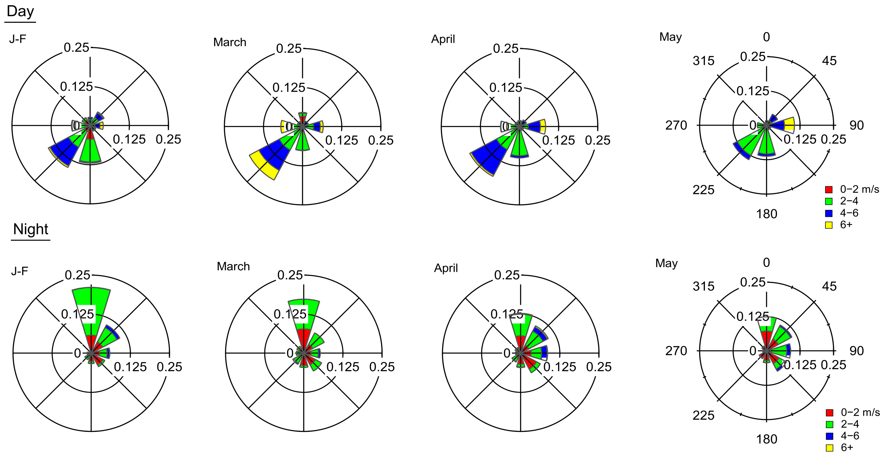
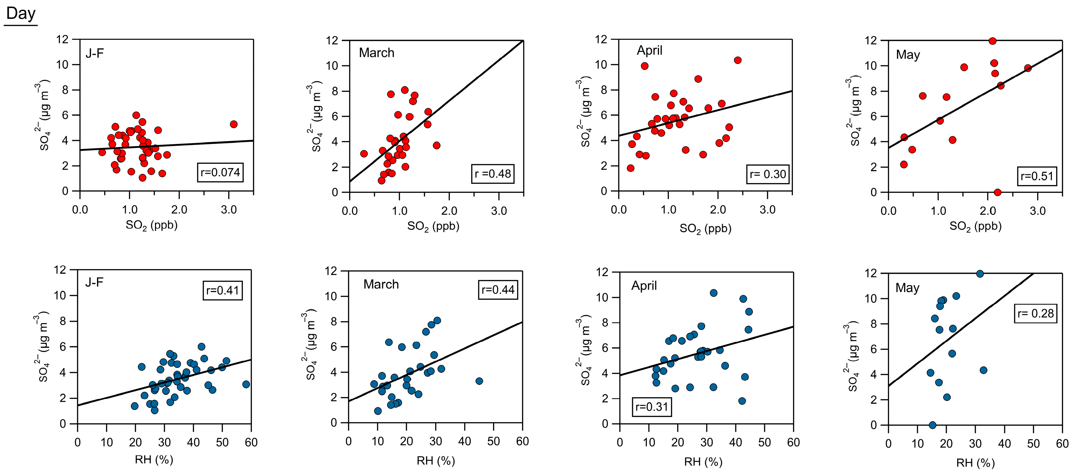
3.1. Meteorology

This study took place during the dry cold season (DC), which includes January and February (J-F), and the dry warm season (DW), which includes March, April, and May, as described by Rozanes-Valenzuela et al. [9] for MAQ. However, to visualize the patterns with greater detail, the analysis and data description were conducted on a monthly basis in Figure 1, which shows the wind roses for each month, both during the day and at nighttime; Figure S2 displays the monthly wind roses using 24 h data. According to Figure 1, the principal wind directions during the day were southwesterly (SW) and southeasterly (SE). The winds with SW directions were more frequent in March and April and less frequent in May. Meanwhile, at night, the wind came mainly from the northwest (NW) and northeast (NE) directions. This local wind pattern matches the regional pattern detailed by Rozanes-Valenzuela et al. [9], who established that the NE and E are the prevailing flows throughout the year; however, during the dry seasons, SW direction flows are also observed. On the other hand, the monthly statistics for T, RH, and WS show an ascending pattern as the year progressed, with an average of 16 °C in J-F (DC) and 23 °C in May (DW) (Figure S3 and Table S1). However, there is no clear trend in RH, although the mean of DC is 47% higher than the mean of DW (Table S1).

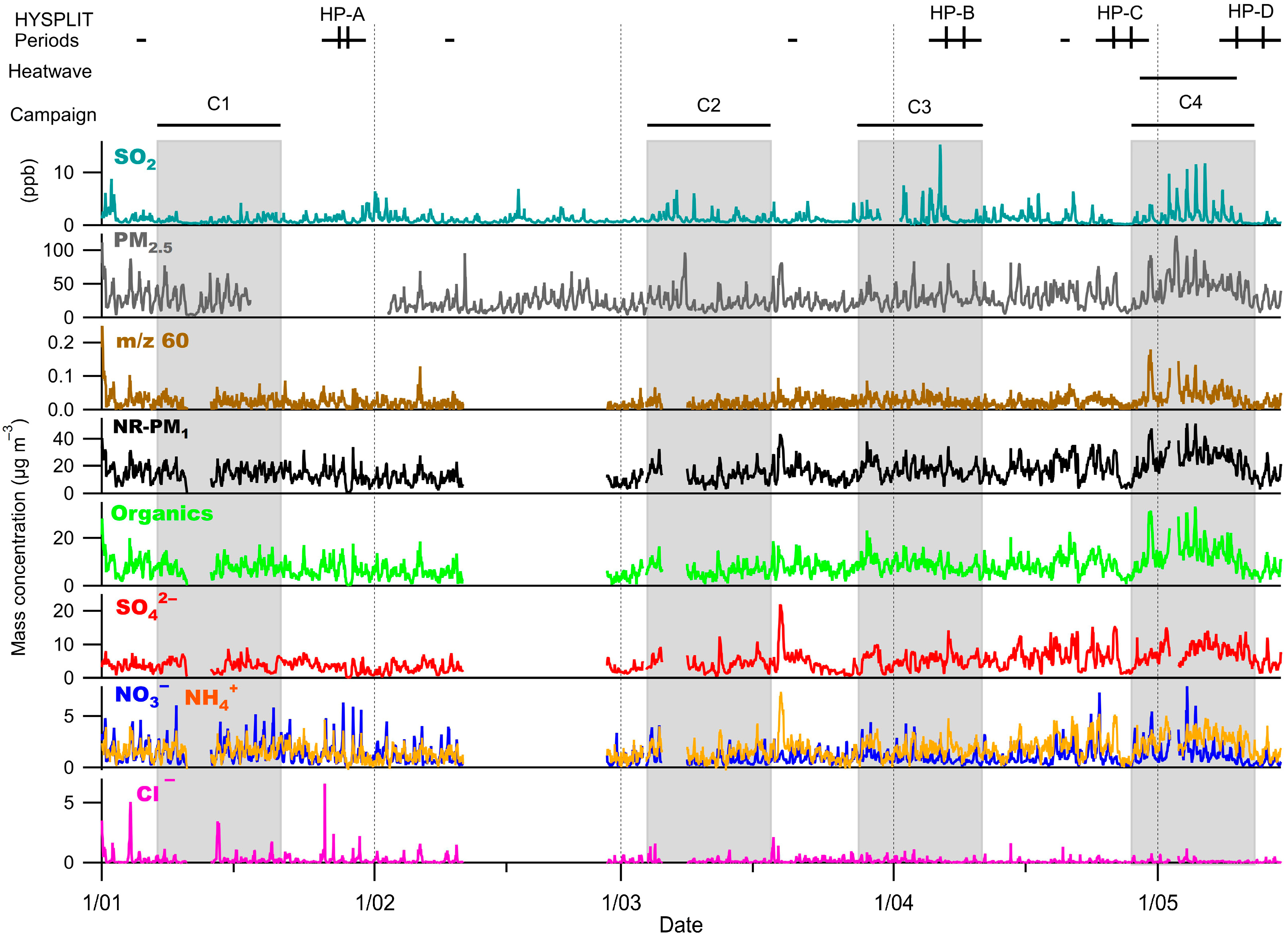
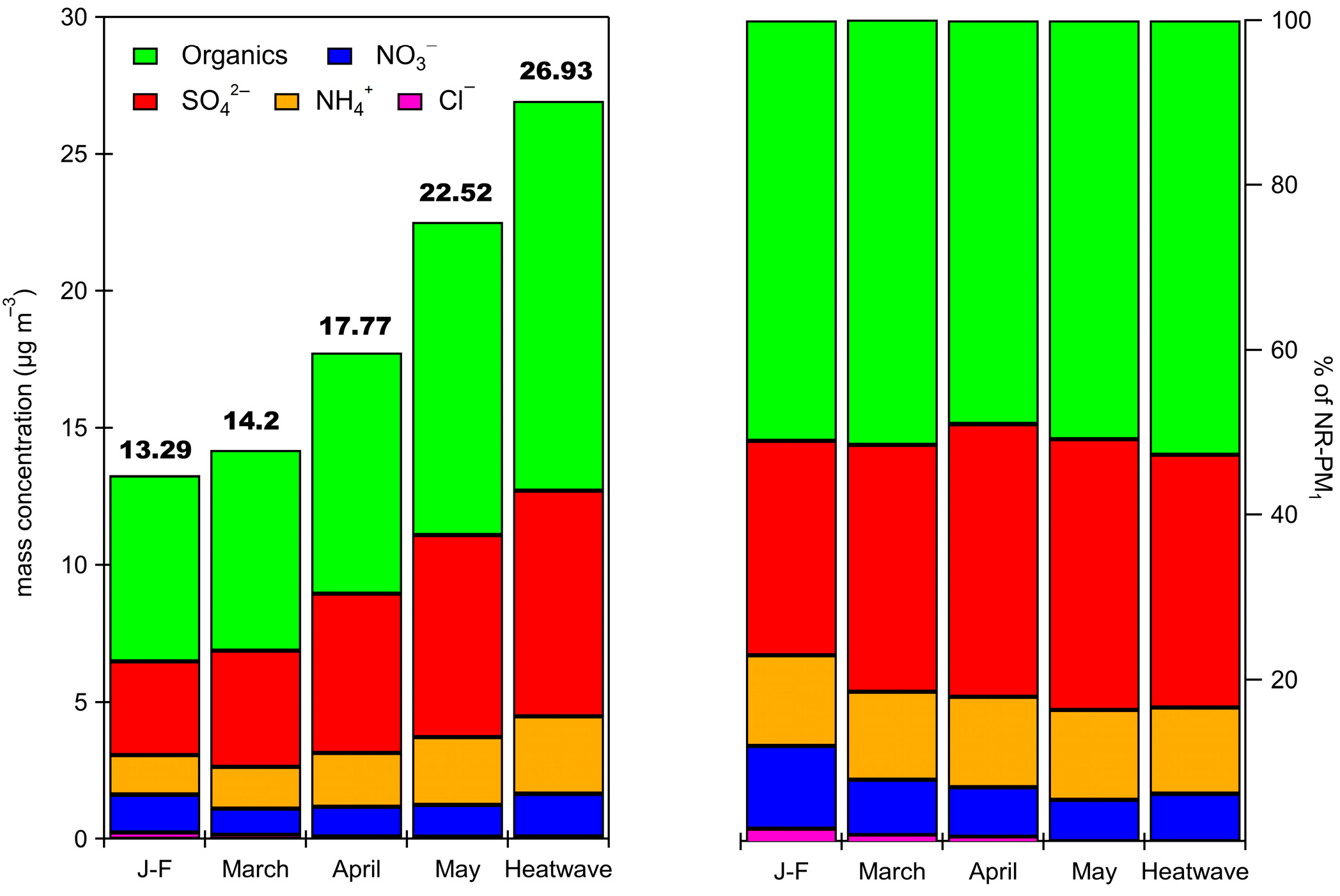
3.2. NR-PM₁ Concentrations and Chemical Composition

The time series of all chemical online data are shown in Figure 2.

Table 3. Summary of the NR-PM₁ composition at the JUR site during this campaign (JUR-2022) and a previous study by Salcedo et al. [11] (JUR-2015). SD corresponding to the standard deviation of each measurement.

	JUR–2022			JUR–2015
	1 January–15 May 2022		Heatwave	1 March 2015–29 February 2016
				DC		DW
	Mean (SD) (µg m−3)	%	Mean (µg m−3)	Mean (SD) (µg m−3)	(%)	Mean (SD) (µg m−3)	%
Organics	8.0 (4.4)	51	14.20 (5.8)	5.4 (3.9)	50	3.3 (2.1)	41
SO42−	4.8 (2.9)	30	8.24 (2.6)	2.7 (1.9)	25	2.9 (1.9)	37
NO3−	1.2 (1.0)	11	1.55 (1.1)	1.2 (1.2)	11	0.6 (0.6)	7.5
NH4+	1.7 (1.0)	7	2.83 (0.9)	1.3 (0.9)	12	1.1 (0.7)	14
Cl−	0.2 (0.4)	1	0.11 (0.2)	0.19 (0.5)	2	0.05 (0.1)	0.6
NR-PM1	15.9 (7.8)	100	26.93 (7.9)	10.8 (6.9)	100	7.9 (4.6)	100

presents the average NR-PM₁ speciated concentration and composition during the whole measurement period, compared with the 2015 data, corresponding to the DC and DW seasons, described by Salcedo et al. [11]. According to this table, the total NR-PM₁ concentrations increased by approximately 58% from 2015 to 2022, mainly due to an increase in the organic fraction and SO₄²⁻ concentrations. In both campaigns, the organic fraction was the main component of the total NR-PM₁ mass, followed by the SO₄²⁻, NO₃⁻, NH₄⁺, and Cl⁻.

3.3. Inorganic Fraction of the NR-PM₁

The monthly speciated mean concentration and composition of NR-PM₁ at the JUR site are shown in Figure 3. In general, the NO₃⁻ and Cl⁻ concentrations were higher during J-F, probably due to a lower height of the boundary layer, which favors their accumulation, as well as low temperatures (Figure S3), which may have favored their partitioning to the condensed phase. Moreover, the diurnal cycles of NO₃⁻ and Cl⁻ concentrations (Figure S4) showed similar diurnal behavior; concentrations increased progressively from 19:00, reaching a maximum between 6:00 and 8:00, which likely corresponds to the minimum height of the boundary layer. Concentrations then showed a steep decrease, with minimal concentrations between 12:00 and 18:00 due to the high volatility of these compounds, which favors their transition to the gas state with the increase in temperature, as well as the deepening of the boundary layer, which redistributes the aerosols to higher altitudes.

Figure 3 shows that the SO₄²⁻ concentrations displayed an ascending pattern during the measurement period, with higher concentrations observed in April and May. This behavior could be associated with an increase in the frequency of SW winds during these months (Section 3.1), which may reflect a greater contribution from regional emissions, given the presence of an important industrial hub in that direction, which includes the Salamanca Refinery (Figure S2). According to Figure S2, March also showed an increase in the frequency of winds coming from the SW. However, SO₄²⁻ concentrations were lower compared to those observed in April and May. This difference is likely due to the relation between RH and SO₄²⁻, which is discussed in more detail in the following paragraphs.

The SO₄²⁻ diurnal cycle (Figure S4) shows a small increase observed during midday, at the highest radiation hours, which may be attributed to local SO₄²⁻ formation from SO₂ oxidation [11] and a decrease in concentration after midday, probably caused by the increased depth the boundary layer, which redistributes the aerosols to higher altitudes.

To further investigate the formation of SO₄²⁻, we consider the relationship between SO₄²⁻ and its precursor SO_2, as well as SO₄²⁻ and RH. Figure 4 presents the scatter plots of their 12 h averages during the day, and Figure S5 shows the corresponding scatter plots for 12 h averages during the night. According to Figure 4, the correlation between SO₂ and SO₄²⁻ was greater during the DW season months (r > 0.4), except in April, when some days with low concentrations of SO₄²⁻ were observed. Some of these days will be described and discussed in more detail in Section 3.7. The good correlation between SO₂ and SO₄²⁻ observed during the DW season, might be related to a more significant regional contribution of both compounds. As described by Rozanes-Valenzuela et al. [9], the high SO₂ concentrations observed in the JUR site during March and April are associated with 50% of the regional flows arriving from the SW, a highly industrialized region which includes the Salamanca Refinery (Figure S2). During the night, the same correlation is very weak (Figure S5), which confirms the contribution of regionally transported air masses rich in SO₂ to the site during the day from the SW region, whereas with the wind shift at night, this correlation disappears. On the other hand, Figure 4 shows that the correlation between RH and SO₄²⁻ concentration decreases through the measurement period. During J-F and March, the correlation between the two variables is higher (r = 0.4) than that observed in April and May (r < 0.3), suggesting a possible local origin of the SO₄²⁻ from January to March, as high RH favors atmospheric oxidation of SO₂ [33].

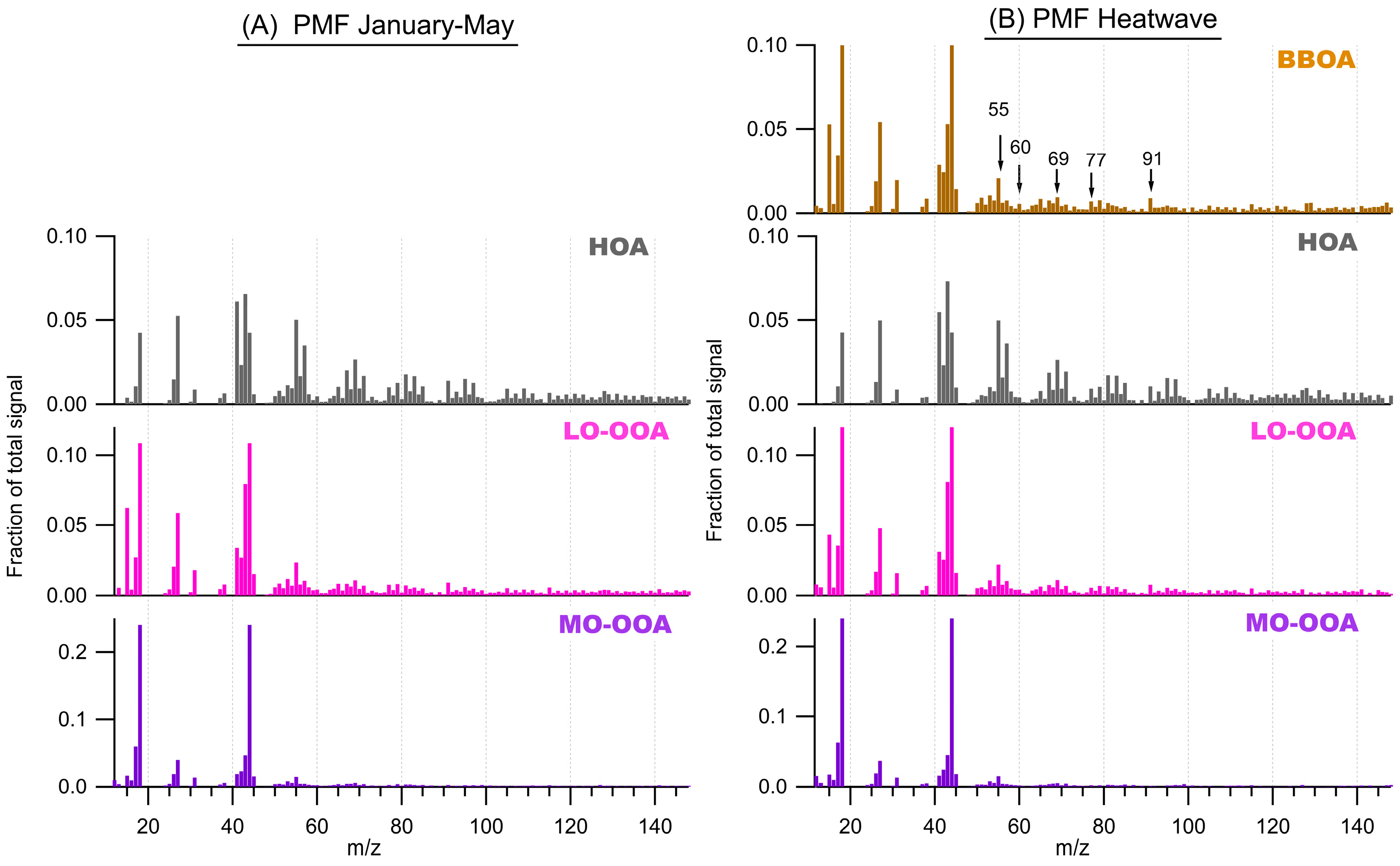
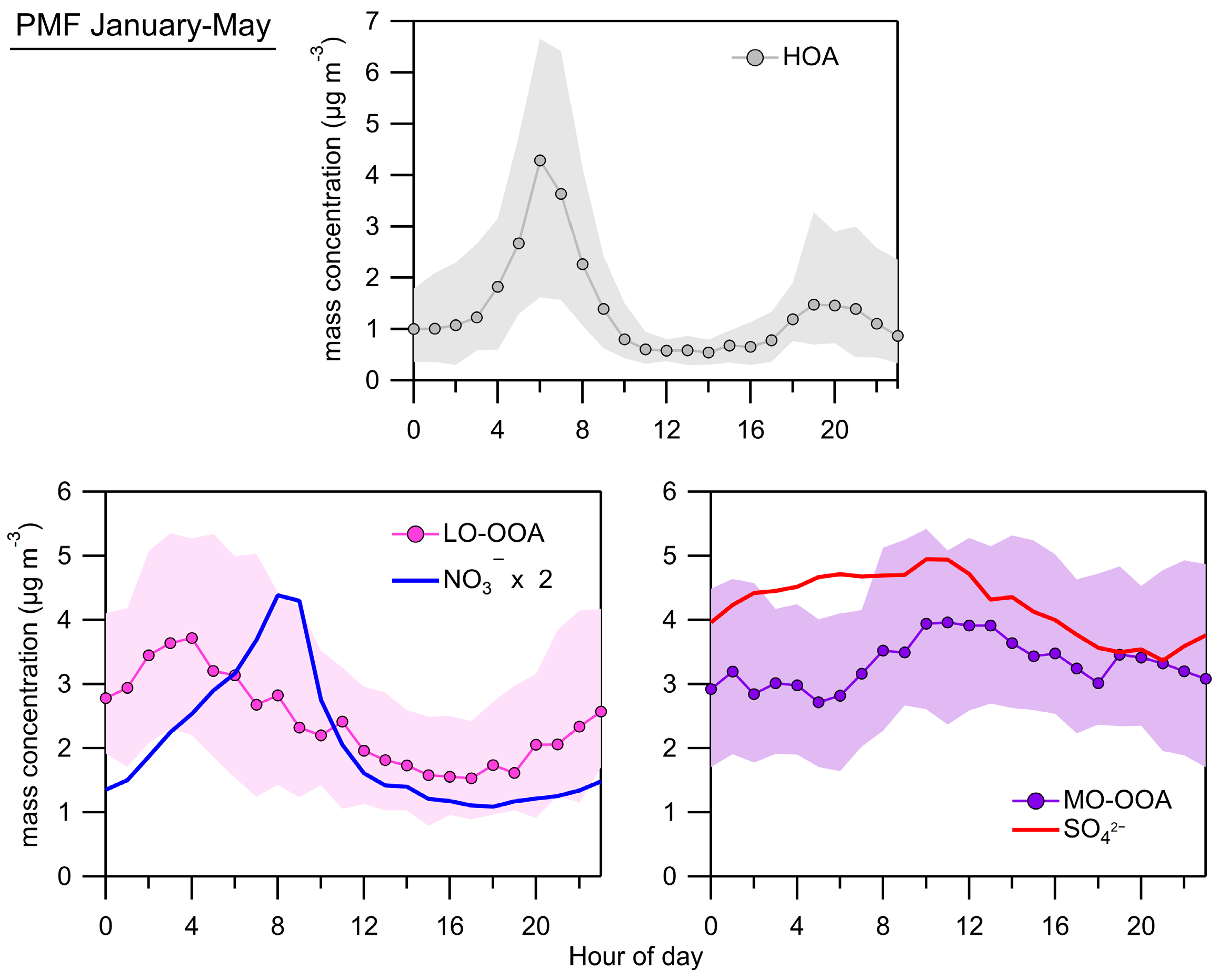
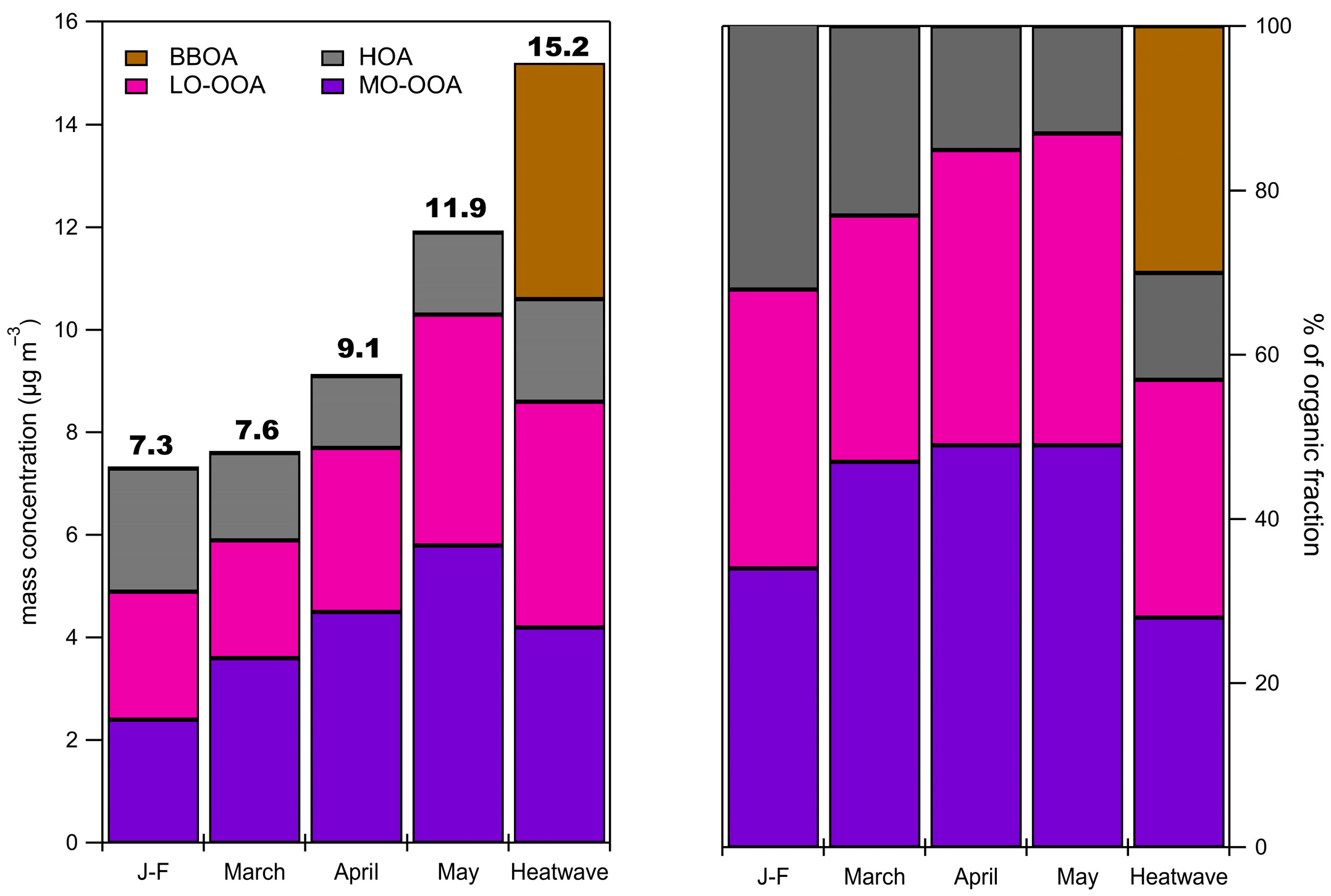
3.4. Organic Fraction of the NR-PM₁

According to Figure S6, which shows the results of the mathematical tools used to choose the best solution, we determined that the three-factor solution of the PMF model adequately reproduced the organic fraction of the NR-PM₁ during the whole measurement period. Figure 5A and Figure 6 show the profiles (mass spectra) and the diurnal cycles, respectively, of the three factors. The three factors corresponded to hydrocarbon-like organic aerosol (HOA), less-oxidized oxygenated organic aerosol (LO-OOA), and more-oxidized oxygenated organic aerosol (MO-OOA), as discussed below. Their time series are shown in Figure S7.

The mass spectrum of the hydrocarbon-like organic aerosol (HOA) profile is characterized by the series C_nH_2n+1 (m/z 29, 43, 57…) and C_nH_2n−1 (m/z 27, 41, 55…) ions, usually identified as hydrocarbons [34,35]. Figure 5A shows that in the HOA profile, the fraction of the total organic signals due to the ions at m/z 43 (f43) and m/z 44 (f44) ions is relatively low (0.06 and 0.04, respectively) in comparison with the values obtained for the LO-OOA and MO-OOA factors (0.08 and 0.15, respectively). This is an indicator of fresh organic compounds since the m/z 44 ion originates mainly from the CO₂⁺ (oxygenated acids) fragment from oxygenated acids, esters, peroxides, etc., whilst the m/z 43 is due to C₂H₃O⁺, a signature of semi-volatile and less oxygenated compounds, such as aldehydes [36]. Therefore, a low value of f44 (i.e., fraction of organic aerosol signal from m/z 44) indicates the presence of compounds that have experienced little oxidation in the atmosphere [37]. The diurnal cycle of the HOA showed two peaks during the day, at 6:00 and around 20:00, which correspond to the hours of maximum vehicular traffic.

The MO-OOA factor mass spectrum was dominated by m/z 44 ion with f44 = 0.24, as observed in Figure 5A. This is a highly oxidized organic aerosol indicator [23,37]. In addition, this factor’s time series has a high correlation with SO₄²⁻ (r = 0.8), and the diurnal cycles of both species are very similar, with relatively constant concentrations during the day, except for a slight increase around midday, which is likely related to local oxidation. Therefore, it is likely that the MO-OOA has a regional source, as does the SO₄²⁻.

The LO-OOA factor mass spectrum showed a f43 value of 0.079, higher than the MO-OOA (f43 = 0.046) factor, and a f44 value of 0.1, lower than the MO-OOA (f44 = 0.24). These values are typical for organic aerosol with a medium oxidation degree, related to local processes and sources [36]. On the other hand, the LO-OOA time series exhibits a high correlation with NO₃⁻ (r = 0.7), and the diurnal cycles of both species follow a similar trend, with concentration increases from 18:00 to the first hours of the next day and low concentrations between 11:00 and 17:00. This correlation suggests that the LO-OOA fraction is semi-volatile, as is the NO₃⁻ [23], this description coincides with reported by Salcedo et al. [11].

Figure 7 shows the contributions of HOA, LO-OOA, and MO-OAA to the total organic fraction measured throughout the study period. The most important component was MO-OOA, whose contribution increased progressively from January to May, from 35% to 49%, likely due to a faster formation of this kind of organic compound associated with an increase in the actinic flux. Table S1 shows an increase of approximately 10% in the radiation daily maximum between J-F and May, and higher regional emissions influence during the months that comprise the DW season, as previously discussed in Section 3.3. The minor component of the organic fraction was HOA; this component’s most significant contribution occurred in J-F and decreased progressively until May. Additionally, the contribution of the LO-OOA component to the organic fraction remained within a small range (30% to 38%) throughout the entire measurement period, slightly increasing towards the end of the period. The results of the PMF model described are consistent with those reported by Salcedo et al. [11].

3.5. Organic Fraction During the Heatwave Period

According to the National Meteorological Service (SMN, Spanish acronym), from 29 April to 10 May, a heatwave occurred over most of the Mexican territory, including the MAQ, which was associated with atmospheric stability. During this period, weak local winds (<4 m/s) were registered at the JUR site, in comparison with previous months (Figure S2). Additionally, an increase in T was observed, accompanied by a decrease in RH (Table S1). This period represents approximately 70% of the data collected for May and will be referred to as “heatwave” in the following sections.

Figure 2 shows that during the heatwave period, an increase in the concentrations of SO₂, organics, NO₃⁻, and the m/z 60 ion was observed, probably due to the accumulation of pollutants in this stagnation period.

We took advantage of this increase to analyze the organic fraction using the PMF model, with the aim of identifying an additional source to the ones described in the previous section. According to Figure S8, which shows the results of mathematical tools used to choose the best solution, we determined that the four-factor model PMF solution adequately reproduced the organic fraction during the heatwave period. Figure 5B shows the profiles of the four factors. According to this figure, three of these factors (MO-OOA, LO-OOA, and HOA) had similar profiles to the ones obtained for the whole measurement period, with a correlation coefficient between 0.95 and 0.99. The fourth factor was identified as Biomass Burning Organic Aerosol (BBOA) because its profile showed a significant contribution, compared to the other factors, of the m/z 60 ion, which is a marker of biomass burning sources [38]. According to Figure S9, which shows the time series of the modeled factors for the heatwave period, the time series of BBOA and m/z 60 ions are similar (r = 0.5). On the other hand, the profile of the BBOA factor showed a contribution from m/z 55, which is associated with food cooking and the presence of fatty acids [39], and m/z 77, 91, and 115, which are markers of coal combustion [36]. Therefore, according to the presence of these tracers, the BBOA factor could also be influenced by cooking organic aerosol (COA). This fourth factor is consistent with the report by Olivares-Salazar et al. [10], who described that, in May 2017, at the JUR site, biomass burning emissions were a source of PM_2.5.

The contributions to the total organic mass from MO-OOA, LO-OOA, and BBOA were 27%, 29%, and 30%, respectively, whilst the HOA contribution was only 14% (Figure 7). More than 80% of the total organic mass had a secondary source, which may indicate local, but continuous, formation of the oxidized aerosol components under atmospheric stability and the heatwave.

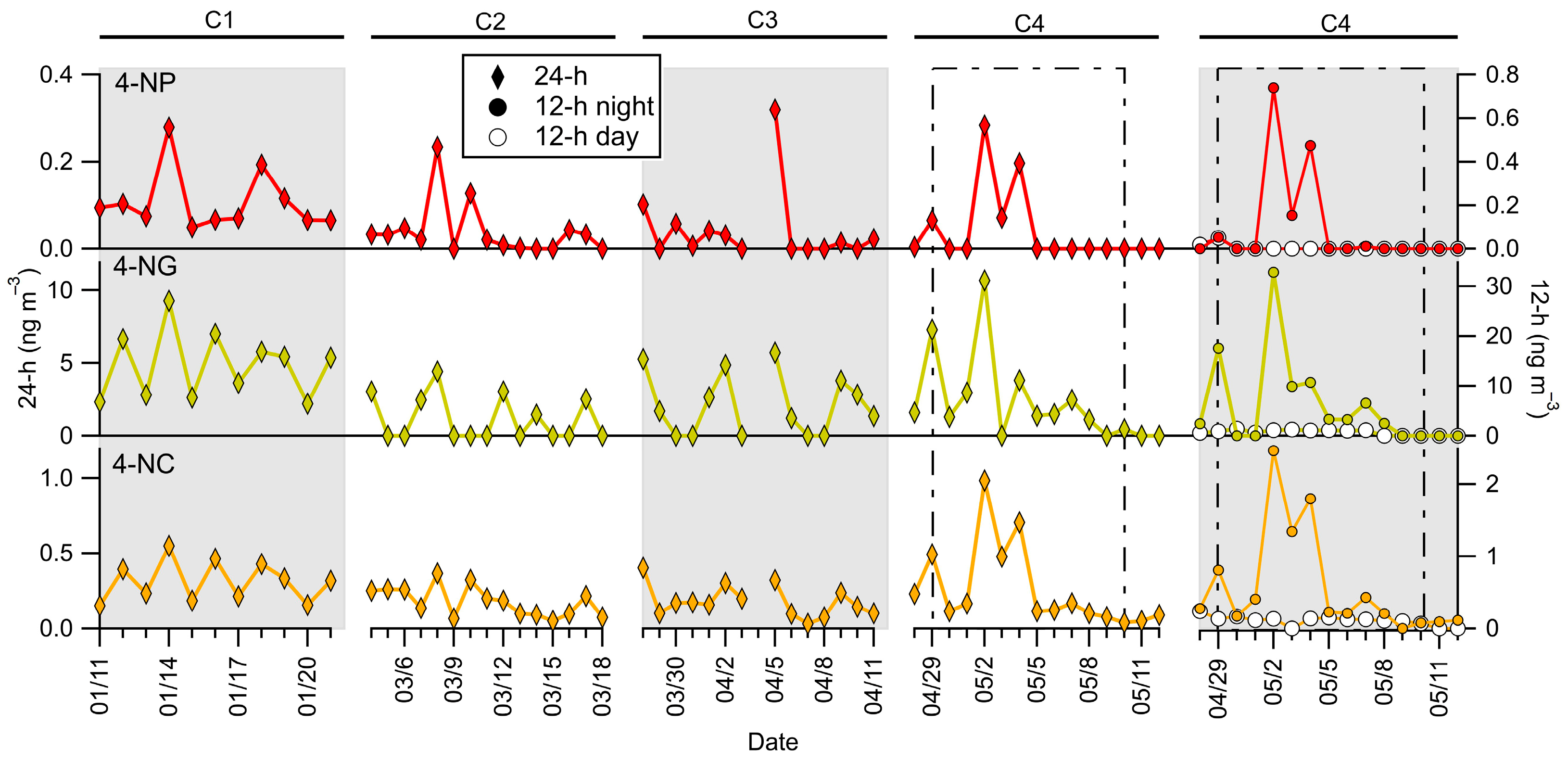
3.6. Nitroaromatic Compounds

Table 4. Average concentration and standard deviation (SD) of NACs, in the 24 h samples, during the four sampling campaigns, the heatwave period, compared to the mean concentration of NACs measured in other sites around the world. BDL: Below Detection Limit.

						Other Sites
	C1	C2	C3	C4	Heatwave	NC-USA [41]	Iowa-USA [40]	Nagoya-Japan [15]
	ng m−3					ng m−3
4-NP	0.10 (0.07)	0.05 (0.06)	0.07 (0.1)	0.12 (0.1)	0.15 (0.1)	0.018–0.12	0.63	--
4-NC	0.31 (0.1)	0.18 (0.1)	0.18 (0.1)	0.26 (0.2)	0.29 (0.3)	0.057–0.16	1.6	0.74–6.8
4-NG	4.83 (2.6)	2.82 (0.9)	3.26 (1.7)	3.13 (3.1)	3.29 (3.2)	-	0.08	0.037–0.55
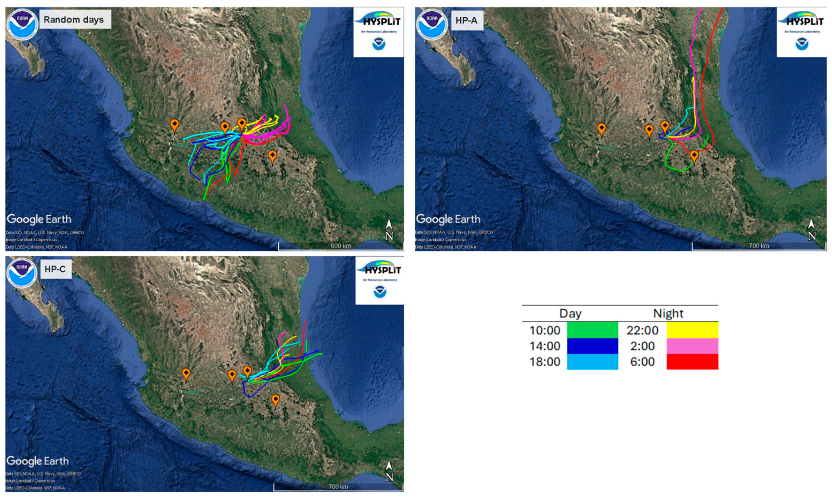
5-NSA	BDL	BDL	BDL	BDL	BDL	-	-	-

presents average concentrations of the four NACs (4-NC, 4-NG, 4-NP, and 5-NSA) quantified in the PM_2.5 samples collected over 24 h or 12 h periods during the four campaigns and the heatwave, which occurred during the C4. The concentration of compound 5-NSA obtained in all the campaigns was below the detection limits (BDL). Ikemori et al. [15] have found that the formation and/or emission of NACs during biomass burning probably depends on the fuel type. A distinction was observed between emissions associated with residential and agricultural activities, with 5-NSA being primarily linked to agricultural practices. In the study area, there is no documented evidence of biomass burning related to agriculture, which may explain why the concentrations of this compound remained below the detection limit in all samples analyzed. Compared to observations in other studies, the 4-NP and 4-NC average concentrations obtained at the JUR site fall within the concentration range reported in other studies conducted in other cities worldwide [15,40,41]. However, in the case of 4-NG, the measured concentrations were approximately 100 times higher. Lauraguais et al. [42] described that nitroguaiacol isomers are tracers for wood combustion; thus, it is likely that high concentrations of 4-NG were related to some undescribed wood-burning source near our study site.

Both in Table 4 and Figure 8, it is observed that 4-NC, 4-NG, and 4-NP during campaigns 1 and 4 are approximately twice as high as those observed in other campaigns. This is probably associated with accumulation processes caused by a lower height of the boundary layer during C1, and by atmospheric stability conditions resulting from the heatwave during C4.

Table 5. Correlations between NAC concentrations and selected measured NR-PM₁ components during the four sampling campaigns. The bold numbers indicate correlations higher than r = 0.7.

	Campaign 1							Campaign 2
	4-NC	4-NG	4-NP	LO-OOA	m/z 60	NO3−	HOA	4-NC	4-NG	4-NP	LO-OOA	m/z 60	NO3−	HOA	BBOA
4-NC	1							1
4-NG	0.98	1						0.44	1
4-NP	0.71	0.70	1					0.78	0.45	1
LO-OOA	0.71	0.67	0.68	1				0.25	0.08	0.23	1
m/z 60	0.72	0.64	0.55	0.67	1			−0.07	0.10	−0.27	0.56	1
NO3	0.47	0.53	0.49	0.56	0.59	1		0.02	0.27	−0.18	0.66	0.85	1
HOA	0.22	0.17	0.08	−0.19	0.39	−0.1	1	0.28	0.50	0.09	0.32	0.48	0.43	1
	Campaign 3								Campaign 4/Heatwave
	4-NC	4-NG	4-NP	LO-OOA	m/z 60	NO3−	HOA	4-NC	4-NG	4-NP	LO-OOA	m/z 60	NO3−	HOA	BBOA
4-NC	1							1
4-NG	0.80	1						0.82	1
4-NP	0.60	0.63	1					0.97	0.78	1
LO-OOA	0.58	0.42	0.28	1				0.87	0.79	0.82	1
m/z 60	0.65	0.42	0.50	0.80	1			0.66	0.65	0.52	0.83	1
NO3	0.82	0.59	0.30	0.84	0.73	1		0.90	0.78	0.80	0.95	0.86	1
HOA	0.74	0.42	0.30	0.74	0.33	0.86	1	0.91	0.83	0.83	0.92	0.74	0.95	1
BBOA								0.82	0.91	0.72	0.84	0.85	0.87	0.86	1

shows the correlation coefficients between the 4-NC, 4-NG, and 4-NP concentrations and the concentrations of other species measured by the ACSM. The data shows a significant correlation (r > 0.6) between the three NACs during campaigns 1, 3, and 4; according to Kahnt et al. [16], this suggests a possible common source of these species. Likewise, in these campaigns, the three NACs concentrations showed a low correlation with the primary compound HOA (r < 0.4), and a moderate to high correlation (r > 0.5) with LO-OOA, NO₃⁻, and the m/z 60 ion. Chow et al. [14] described that a good correlation between NACs and secondary species, such as NO₃⁻, suggests a secondary source for NACs. Considering that LO-OOA and NO₃⁻ have a local origin, it is reasonable to consider that precursors for NACs are also emitted locally. Furthermore, according to Kahnt et al. [16], the high correlation between NACs and m/z 60 ions indicates that their origin is likely related to biomass burning. Therefore, it is probable that NACs, within the MAQ, had a secondary origin associated with biomass burning emissions.

During C4, a significant correlation (r > 0.6) was observed among all species (Table 5), probably due to the general concentration enhancements and the atmospheric stability caused by the heatwave. Figure 8 shows the NAC concentration time series in the samples collected every 12 hours (day and night). We observed that nighttime concentrations of 4-NP, 4-NC, and 4-NG were much higher than during the day, with the latter generally being below the MDL in most samples. Wu et al. [43] described that low T and high RH conditions could favor aerosol formation through the gas-phase oxidation of volatile organic compounds emitted by biomass burning, in the presence of NO₃⁻ radicals. Such T and RH conditions were observed during nighttime at the JUR site, which might explain the higher nocturnal concentrations of NACs compared to those observed during the daytime.

3.7. HYSPLIT Model

We identified four periods when the NO₃⁻, SO₄²⁻, and the organic fraction of NR-PM₁ concentrations were very low (between 30 to 50% below average), which are marked in Figure 2 as H-P A to D. No difference was identified between the local meteorological conditions during those periods, compared to a few days before or after. Hence, back trajectories obtained with the HYSPLIT during these periods were analyzed to identify potential changes in regional wind flow patterns that could have caused such changes in concentrations. To establish a reference pattern of back trajectories for comparison, trajectories were also modeled for two days before and after such periods, as well as for randomly selected days throughout the entire measurement period.

Table 6. List of periods with very low concentrations for which back trajectories were obtained using the HYSPLIT model.

	HYSPLIT Modeling Period	Reference Periods
		Previous Days	Subsequent Days
HP-A	28 January, 13:00 to 29, 12:00	26–27 January	30–31 January
HP-B	7 April, 06:00 to 9, 23:00	4–5 April	10–11 April
HP-C	26 April, 08:00 to 28, 09:00	24–25 April	29–30 April
HP-D	10 May, 12:00 to 13, 05:00	8–9 May	14–15 May
Random days	5 January, 9 February, 20 March, 20 April, 4 May

lists all the dates for which back trajectories were calculated, which are also shown in Figure 2.

Figure 9 shows the reference back trajectories, considering only random days, and for periods HP-A and HP-C, while Figure S10 shows the back trajectories of the HP-B and HP-D periods, whose patterns were very similar, and Figure S11 shows the trajectories obtained from days before and after the periods of minimum concentration. According to Figure 9, during the reference periods, nighttime trajectories arrived at the JUR site mainly from the N and NE, and in the daytime from the SW and NW. However, during the HP-A and HP-C periods, trajectories arrived only from the N-NE direction in both day and night times. These results indicate that the absence of regional flows from W or SW directly (where an important industrial hub is located) resulted in a lower concentration of the main component of NR-PM₁ (organic fraction). Our observations indicate that regional emissions have a significant impact on the concentration and chemical composition of aerosols at the JUR site.

4. Conclusions

During 1 January to 15 May 2022, at MAQ, the source apportionment results for the organic fraction of NR-PM₁ showed three factors: HOA, LO-OOA, and MO-OOA. Aged aerosols (MO-OOA and SO₄²⁻) accounted for approximately 40% of the total NR-PM₁ mass, representing its main component. The increase in the concentration of these aerosols during the DW season (100% increase) was associated with a higher frequency of regional winds originating from the W and SW, where a major industrial area is located, and a faster aging associated with an increase in the actinic flux. Conversely, the absence of regional flows from the W and SW directions was associated with a significant decrease (30–50%) in the organic fraction of NR-PM₁. On the other hand, an additional factor of the organic fraction associated with biomass burning (BBOA) was identified during the heatwave period, which was likely enhanced by the accumulation of atmospheric pollutants under stable conditions. The BBOA emissions were also described by quantifying NAC concentrations in the MAQ for the first time. Our results indicate a predominantly secondary origin of NACs, related to the oxidation of VOCs emitted during biomass and wood burning. The highest atmospheric concentrations of NACs (0.1 to 4.8 ng m⁻³) were observed during the DC season and the heatwave period, characterized by pollutant accumulation events.

Our results highlight the critical role that regional meteorology plays in determining the concentration and chemical composition of the atmospheric aerosol in the MAQ. First, the atmospheric stability associated with developing a heatwave facilitated the accumulation of pollutants during the heatwave period, allowing for the identification and quantification of previously unreported emission sources. Second, a shift in regional air mass flows notably impacted the NR-PM₁ concentrations, particularly in their organic fraction.

Therefore, we emphasize the need to develop targeted studies to identify additional aerosol emission sources, especially those linked to industrial activities, given that the MAQ is located in El Bajío, Mexico’s most important industrial region. Moreover, the results presented here should be considered in the design and implementation of air pollution control strategies and emission regulations.

References

1. WHO. Ambient (Outdoor) Air Pollution. Available online: https://www.who.int/news-room/fact-sheets/detail/ambient-(outdoor)-air-quality-and-health (accessed on 20 February 2025).
2. Wu, S.; Deng, F.; Wei, H.; Huang, J.; Wang, X.; Hao, Y.; Zheng, C.; Qin, Y.; Lv, H.; Shima, M.; et al. Association of Cardiopulmonary Health Effects with Source-Appointed Ambient Fine Particulate in Beijing, China: A Combined Analysis from the Healthy Volunteer Natural Relocation (HVNR) Study. Environ. Sci. Technol. 2014, 48, 3438–3448. [Google Scholar] [CrossRef]
3. Terzano, C.; Di Stefano, F.; Conti, V.; Graziani, E.; Petroianni, A. Air Pollution Ultrafine Particles: Toxicity beyond the Lung. Eur. Rev. Med. Pharmacol. Sci. 2010, 14, 809–821. [Google Scholar]
4. Brook, R.D.; Rajagopalan, S.; Pope, C.A.; Brook, J.R.; Bhatnagar, A.; Diez-Roux, A.V.; Holguin, F.; Hong, Y.; Luepker, R.V.; Mittleman, M.A.; et al. Particulate Matter Air Pollution and Cardiovascular Disease: An Update to the Scientific Statement from the American Heart Association. Circulation 2010, 121, 2331–2378. [Google Scholar] [CrossRef]
5. Cachon, B.F.; Firmin, S.; Verdin, A.; Ayi-Fanou, L.; Billet, S.; Cazier, F.; Martin, P.J.; Aissi, F.; Courcot, D.; Sanni, A.; et al. Proinflammatory Effects and Oxidative Stress within Human Bronchial Epithelial Cells Exposed to Atmospheric Particulate Matter (PM2.5 and PM>2.5) Collected from Cotonou, Benin. Environ. Pollut. 2014, 185, 340–351. [Google Scholar] [CrossRef]
6. IPCC. Clouds and Aerosols. In Climate Change 2013—The Physical Science Basis; Intergovernmental Panel on Climate Change, Ed.; Cambridge University Press: Cambridge, UK, 2013; pp. 571–658. [Google Scholar] [CrossRef]
7. Koplik, E.V.; Umriukhin, P.E.; Konorova, I.L.; Terechina, O.L.; Michaleva, I.I.; Gannushkina, I.V.; Sudakov, K.V. Atmospheric Aerosols: Composition, Transformation, Climate and Health Effects. Zhurnal Nevrol. I Psihiatr. Im. S S Korsakova 2007, 107, 50–54. [Google Scholar] [CrossRef]
8. Molina, L.T.; Madronich, S.; Gaffney, J.S.; Apel, E.; De Foy, B.; Fast, J.; Ferrare, R.; Herndon, S.; Jimenez, J.L.; Lamb, B.; et al. An Overview of the MILAGRO 2006 Campaign: Mexico City Emissions and Their Transport and Transformation. Atmos. Chem. Phys. 2010, 10, 8697–8760. [Google Scholar] [CrossRef]
9. Rozanes-Valenzuela, D.A.; Magaldi, A.V.; Salcedo, D. Regional Flow Climatology for Central Mexico (Querétaro): A First Case Study. Atmosfera 2023, 36, 239–252. [Google Scholar] [CrossRef]
10. Olivares-Salazar, S.E.; Alvarez-Ospina, H.; Aguillon-Vazquez, C.; Salcedo, D. Source Apportionment of Particulate Matter in the Metropolitan Area of Querétaro (Central Mexico): First Case Study. ACS Earth Space Chem. 2021, 5, 2347–2355. [Google Scholar] [CrossRef]
11. Salcedo, D.; Alvarez-Ospina, H.; Olivares-Salazar, S.E.; Liñan-Abanto, R.N.; Castro, T. PM Chemical Characterization at a Semi-Arid Urban Environment in Central Mexico. Urban Clim. 2023, 52, 101723. [Google Scholar] [CrossRef]
12. Bejan, I.G.; Olariu, R.I.; Wiesen, P. Secondary Organic Aerosol Formation from Nitrophenols Photolysis under Atmospheric Conditions. Atmosphere 2020, 11, 1346. [Google Scholar] [CrossRef]
13. Tremp, J.; Mattrel, P.; Fingler, S.; Giger, W. Phenols and Nitrophenols as Tropospheric Pollutants: Emissions from Automobile Exhausts and Phase Transfer in the Atmosphere. Water Air Soil Pollut. 1993, 68, 113–123. [Google Scholar] [CrossRef]
14. Chow, K.S.; Huang, X.H.H.; Yu, J.Z. Quantification of Nitroaromatic Compounds in Atmospheric Fine Particulate Matter in Hong Kong over 3 Years: Field Measurement Evidence for Secondary Formation Derived from Biomass Burning Emissions. Environ. Chem. 2016, 13, 665–673. [Google Scholar] [CrossRef]
15. Ikemori, F.; Nakayama, T.; Hasegawa, H. Characterization and Possible Sources of Nitrated Mono- and Di-Aromatic Hydrocarbons Containing Hydroxyl and/or Carboxyl Functional Groups in Ambient Particles in Nagoya, Japan. Atmos. Environ. 2019, 211, 91–102. [Google Scholar] [CrossRef]
16. Kahnt, A.; Behrouzi, S.; Vermeylen, R.; Safi Shalamzari, M.; Vercauteren, J.; Roekens, E.; Claeys, M.; Maenhaut, W. One-Year Study of Nitro-Organic Compounds and Their Relation to Wood Burning in PM10 Aerosol from a Rural Site in Belgium. Atmos. Environ. 2013, 81, 561–568. [Google Scholar] [CrossRef]
17. Malagón, A. Directorio Empresarial PIQ. 2025. Available online: https://www.piq.com.mx/files/DIRECTORIO_EMPRESAS_PIQ_FEBRERO_2025.pdf (accessed on 18 May 2025).
18. Red Universitaria De Observatorio Atmosféricos. RUOA. Available online: https://ruoa.unam.mx/estaciones/jqro/ (accessed on 18 May 2025).
19. Jimenez, J.L.; Jayne, J.T.; Shi, Q.; Kolb, C.E.; Worsnop, D.R.; Yourshaw, I.; Seinfeld, J.H.; Flagan, R.C.; Zhang, X.; Smith, K.A.; et al. Ambient Aerosol Sampling Using the Aerodyne Aerosol Mass Spectrometer. J. Geophys. Res. Atmos. 2003, 108, 1–13. [Google Scholar] [CrossRef]
20. Ng, N.L.; Herndon, S.C.; Trimborn, A.; Canagaratna, M.R.; Croteau, P.L.; Onasch, T.B.; Sueper, D.; Worsnop, D.R.; Zhang, Q.; Sun, Y.L. An aerosol chemical speciation monitor (ACSM) for routine monitoring of the composition and mass concentrations of ambient aerosol. Aerosol. Sci. Technol. 2011, 45, 780–794. [Google Scholar] [CrossRef]
21. Canagaratna, M.R.; Jayne, J.T.; Jimenez, J.L.; Allan, J.D.; Alfarra, M.R.; Zhang, Q.; Onasch, T.B.; Drewnick, F.; Coe, H.; Middlebrook, A.; et al. Chemical and Microphysical Characterization of Ambient Aerosols with the Aerodyne Aerosol Mass Spectrometer. Mass Spectrom. Rev. 2007, 2, 185–222. [Google Scholar] [CrossRef]
22. Paatero, P.; Tappert, U. Positive Matrix Factorization: A Non-Negative Factor Model with Optimal Utilization of Error Estimates of Data Values. Environmetrics 1994, 5, 111–126. [Google Scholar] [CrossRef]
23. Ulbrich, I.M.; Canagaratna, M.R.; Zhang, Q.; Worsnop, D.R.; Jimenez, J.L. Interpretation of Organic Components from Positive Matrix Factorization of Aerosol Mass Spectrometric Data. Atmos. Chem. Phys. 2009, 9, 2891–2918. [Google Scholar] [CrossRef]
24. Hopke, P.K. Review of Receptor Modeling Methods for Source Apportionment. J. Air Waste Manag. Assoc. 2016, 66, 237–259. [Google Scholar] [CrossRef] [PubMed]
25. Paatero, P. User’s Guide for the Multilinear Engine Program “ME2” for Fitting Multilinear and Quasi-Multilinear Models; University of Helsinki, Department of Physics: Helsinki, Finland, 2000; pp. 1–24. [Google Scholar]
26. Zhang, Q.; Jimenez, J.L.; Canagaratna, M.R.; Ulbrich, I.M.; Ng, N.L.; Worsnop, D.R.; Sun, Y. Understanding Atmospheric Organic Aerosols via Factor Analysis of Aerosol Mass Spectrometry: A Review. Anal. Bioanal. Chem. 2011, 401, 3045–3067. [Google Scholar] [CrossRef]
27. Jiang, H.; Frie, A.L.; Lavi, A.; Chen, J.Y.; Zhang, H.; Bahreini, R.; Lin, Y.H. Brown Carbon Formation from Nighttime Chemistry of Unsaturated Heterocyclic Volatile Organic Compounds. Environ. Sci. Technol. Lett. 2019, 6, 184–190. [Google Scholar] [CrossRef]
28. Cui, Y.; Chen, K.; Zhang, H.; Lin, Y.-H.; Bahreini, R. Chemical Composition and Optical Properties of Secondary Organic Aerosol from Photooxidation of Volatile Organic Compound Mixtures. ACS EST Air 2024, 1, 247–258. [Google Scholar] [CrossRef]
29. Kitanovski, Z.; Grgić, I.; Vermeylen, R.; Claeys, M.; Maenhaut, W. Liquid Chromatography Tandem Mass Spectrometry Method for Characterization of Monoaromatic Nitro-Compounds in Atmospheric Particulate Matter. J. Chromatogr. A 2012, 1268, 35–43. [Google Scholar] [CrossRef]
30. Gegenschatz, S.A.; Chiappini, F.A.; Teglia, C.M.; de la Peña, A.M.; Goicoechea, H.C. Binding the Gap between Experiments, Statistics, and Method Comparison: A Tutorial for Computing Limits of Detection and Quantification in Univariate Calibration for Complex Samples. Anal. Chim. Acta 2021, 1209, 339342. [Google Scholar] [CrossRef]
31. Rolph, G.; Stein, A.; Stunder, B. Real-Time Environmental Applications and Display SYstem: READY. Environ. Model. Softw. 2017, 95, 210–228. [Google Scholar] [CrossRef]
32. Stein, A.F.; Draxler, R.R.; Rolph, G.D.; Stunder, B.J.B.; Cohen, M.D.; Ngan, F. NOAA’s HYSPLIT Atmospheric Transport and Dispersion Modeling System. Bull. Am. Meteorol. Soc. 2015, 96, 2059–2077. [Google Scholar] [CrossRef]
33. Seinfeld, J.H.; Pandis, S.N. Atmospheric Chemistry and Physics from Air Pollution to Climate Change, 2nd ed.; Publication; John Wiley & Sons, Inc.: Hoboken, NJ, USA, 2006. [Google Scholar]
34. Zhang, Q.; Canagaratna, M.R.; Jayne, J.T.; Worsnop, D.R.; Jimenez, J.L. Time- and Size-Resolved Chemical Composition of Submicron Particles in Pittsburgh: Implications for Aerosol Sources and Processes. J. Geophys. Res. Atmos. 2005, 110, 1–19. [Google Scholar] [CrossRef]
35. Lanz, V.A.; Alfarra, M.R.; Baltensperger, U.; Buchmann, B.; Hueglin, C.; Prévôt, A.S.H. Source Apportionment of Submicron Organic Aerosols at an Urban Site by Factor Analytical Modelling of Aerosol Mass Spectra. Atmos. Chem. Phys. 2007, 7, 1503–1522. [Google Scholar] [CrossRef]
36. Atabakhsh, S.; Poulain, L.; Chen, G.; Canonaco, F.; Prévôt, A.S.H.; Pöhlker, M.; Wiedensohler, A.; Herrmann, H. A 1-Year Aerosol Chemical Speciation Monitor (ACSM) Source Analysis of Organic Aerosol Particle Contributions from Anthropogenic Sources after Long-Range Transport at the TROPOS Research Station Melpitz. Atmos. Chem. Phys. 2023, 23, 6963–6988. [Google Scholar] [CrossRef]
37. Ng, N.L.; Canagaratna, M.R.; Zhang, Q.; Jimenez, J.L.; Tian, J.; Ulbrich, I.M.; Kroll, J.H.; Docherty, K.S.; Chhabra, P.S.; Bahreini, R.; et al. Organic Aerosol Components Observed in Northern Hemispheric Datasets from Aerosol Mass Spectrometry. Atmos. Chem. Phys. 2010, 10, 4625–4641. [Google Scholar] [CrossRef]
38. Simoneit, B.R.T.; Schauer, J.J.; Nolte, C.G.; Oros, D.R.; Elias, V.O.; Fraser, M.P.; Rogge, W.F.; Cass, G.R. Levoglucosan, a Tracer for Cellulose in Biomass Burning and Atmospheric Particles. Atmos. Environ. 1999, 33, 173–182. [Google Scholar] [CrossRef]
39. Jeon, S.; Walker, M.J.; Sueper, D.T.; Day, D.A.; Handschy, A.V.; Jimenez, J.L.; Williams, B.J. A Searchable Database and Mass Spectral Comparison Tool for Aerosol Mass Spectrometry (AMS) and Aerosol Chemical Speciation Monitor (ACSM). EGUsphere 2023, 16, 6075–6095. [Google Scholar] [CrossRef]
40. Al-Naiema, I.M.; Stone, E.A. Evaluation of Anthropogenic Secondary Organic Aerosol Tracersfrom Aromatic Hydrocarbons. Atmos. Chem. Phys. 2017, 17, 2053–2065. [Google Scholar] [CrossRef]
41. Xie, M.; Chen, X.; Holder, A.L.; Hays, M.D.; Lewandowski, M.; Offenberg, J.H.; Kleindienst, T.E.; Jaoui, M.; Hannigan, M.P. Light Absorption of Organic Carbon and Its Sources at a Southeastern U.S. Location in Summer. Environ. Pollut. 2018, 244, 38–46. [Google Scholar] [CrossRef]
42. Lauraguais, A.; Coeur-Tourneur, C.; Cassez, A.; Deboudt, K.; Fourmentin, M.; Choël, M. Atmospheric Reactivity of Hydroxyl Radicals with Guaiacol (2-Methoxyphenol), a Biomass Burning Emitted Compound: Secondary Organic Aerosol Formation and Gas-Phase Oxidation Products. Atmos. Environ. 2014, 86, 155–163. [Google Scholar] [CrossRef]
43. Wu, C.; Zhang, S.; Wang, G.; Lv, S.; Li, D.; Liu, L.; Li, J.; Liu, S.; Du, W.; Meng, J.; et al. Efficient Heterogeneous Formation of Ammonium Nitrate on the Saline Mineral Particle Surface in the Atmosphere of East Asia during Dust Storm Periods. Environ. Sci. Technol. 2020, 54, 15622–15630. [Google Scholar] [CrossRef]
Figure 1. Monthly wind roses for day (10:00 to 22:00) and nighttime (22:00 to 10:00 next day). The axial scale represents the frequency of wind coming from a specific direction.
Atmosphere 16 00827 g001
Figure 2. Time series of all chemical online data at JUR during the measurement period. The equivalent mass concentration of the ion m/z 60 is also shown. The gray areas highlight the four off-line sampling campaigns (Table 1). The heatwave period and the periods modeled with HYSPLIT are also marked on the top of the figure with horizontal lines.
Atmosphere 16 00827 g002
Figure 3. Monthly means speciated concentration and composition of NR-PM1 measured by ACSM. The sum of the organics, SO42−, NO3, NH4+, and Cl concentrations corresponds to the total mass concentration of NR-PM1 (bold numbers). The heatwave period is also shown.
Atmosphere 16 00827 g003
Figure 4. Scatter plots of 12 h SO42− concentration during the day (10:00–22:00) vs. SO2 (red dots) and RH (blue dots). Black lines represent the linear fit, and r is the Pearson correlation coefficient.
Atmosphere 16 00827 g004
Figure 5. Profiles (mass spectrum) of the PMF organic factors for (A) the whole measurement period (PMF January–May), and (B) the heatwave period (PMF heatwave).
Atmosphere 16 00827 g005
Figure 6. Average diurnal profiles of the three organic factors (lines + dots), compared to other species (continuous lines), at JUR for the whole measured period. The shadows represent the interquartile range of concentrations. NO3 profile shown is multiplied by a factor of 2 to facilitate visual comparison.
Atmosphere 16 00827 g006
Figure 7. Monthly means speciated concentration and composition of the organic fraction of NR-PM1. The sum of the HOA, LO-OOA, MO-OOA, and BBOA concentrations corresponds to the organic fraction’s total mass (bold numbers). The heatwave period is also shown.
Atmosphere 16 00827 g007
Figure 8. NAC concentrations in PM2.5 samples. For C4, 24 h and 12 h concentrations are shown. The dotted lines mark the heatwave period.
Atmosphere 16 00827 g008
Figure 9. HYSPLIT retro-trajectories for the random days and HP-A and C periods (Table 6). Each trajectory was traced back for twelve hours in time. The table shows the arrival time of the trajectories at the JUR site. Markers represent the same sites shown in Figure S1 (MAQ, GDL, SR, MCMA).
Atmosphere 16 00827 g009