Enhancing Typhoon Doksuri (2023) Forecasts via Radar Data Assimilation: Evaluation of Momentum Control Variable Schemes with Background-Dependent Hydrometeor Retrieval in WRF-3DVAR

Abstract

This research investigates how incorporating both radar radial velocity ($V_r$) and radar reflectivity influences the accuracy of tropical cyclone (TC) prediction. Different control variables are introduced to analyze their roles in $V_r$ data assimilation, while background-dependent radar reflectivity assimilation methods are also applied. Using Typhoon “Doksuri” (2023) as a primary case study and Typhoon “Kompasu” (2021) as a supplementary case, the Weather Research and Forecasting (WRF) model’s three-dimensional variational assimilation (3DVAR) is utilized to assimilate $V_r$ and reflectivity observations to improve TC track, intensity, and precipitation forecasts. Three experiments were conducted for each typhoon: one with no assimilation, one with $V_r$ assimilation using $\psi -\chi$ control variables and background-dependent radar reflectivity assimilation, and one with $V_r$ assimilation using $U-V$ control variables and background-dependent radar reflectivity assimilation. The results show that assimilating $V_r$ enhances small-scale dynamics in the TC core, leading to a more organized and stronger wind field. The experiment involving $U-V$ control variables consistently showed advantages over the $\psi -\chi$ scheme in aspects such as overall track prediction, initial intensity representation, and producing more stable or physically plausible intensity trends, particularly evident when comparing both typhoon events. These findings highlight the importance of optimizing control variables and assimilation methods to enhance the prediction of TCs.

1. Introduction

Tropical cyclones (TCs) are recognized as some of the most devastating natural disasters worldwide, posing significant threats, especially to coastal areas, where their intense winds and heavy rainfall frequently lead to catastrophic loss of people’s lives and property [1]. Progress in data assimilation (DA) techniques, coupled with the integration of higher-resolution four-dimensional observations—such as radar data—have substantially enhanced the forecasting of tropical cyclone tracks and intensity [2,3,4,5,6,7,8,9,10,11,12,13,14]. Accurate forecasting of TC tracks, intensity, and precipitation is critical for mitigating these impacts. However, predicting the intensity of tropical cyclones continues to pose a significant challenge due to the complex dynamic and thermodynamic characteristics governing the inner core structure of the TC. Errors in initial conditions, compounded by the limited availability of observational data, often introduce substantial biases, complicating precise prediction of TC intensity.

Recent advancements in observational technologies have provided high-resolution data that can markedly enhance the accuracy of TC forecasts. Among these, radar data are crucial for capturing detailed information on the wind field structure within TCs, particularly in the inner core. Specifically, incorporating hydrometeor control variables into radar data assimilation schemes has been demonstrated to enhance precipitation forecasts and provide a more accurate representation of inner-core structures [5]. Assimilating such high-resolution data into numerical weather prediction (NWP) models enables better representation of TC dynamics and thermodynamics characteristics. This improves the initial conditions and, consequently, the precision of forecasts for TC track, intensity, and rainfall predictions. Earlier research has highlighted the effectiveness of assimilating methods like the Ensemble Kalman Filter (EnKF) into NWP models; this ensemble-based data assimilation enables assimilation of inner-core observations at convection-allowing resolutions for TC initialization [15,16,17,18]. Additionally, Lei et al. (2018) demonstrated that implementing model space localization in EnKF improves assimilation of radiance observations, which could offer insights for enhancing the assimilation of radar data in tropical cyclone forecasting [19]. Furthermore, Bishop and Hodyss (2007) [20] proposed a flow-adaptive moderation approach (SENCORP) to mitigate spurious ensemble correlations arising from limited ensemble size, a key limitation of EnKF frameworks. This technique provides a foundation for further improving the robustness and accuracy of ensemble-based assimilation, especially in the presence of flow-dependent correlation structures. By assimilating radar radial velocity ($V_r$), the ensemble–variational DA system notably enhanced forecasts for Hurricane Ike (2008). This approach better represented the small-scale dynamics of the hurricane, and the assimilation of radar data led to substantial improvements in the hurricane’s intensity, track, and precipitation forecasts compared to experiments without radar data assimilation [4]. Assimilating reflectivity along with conventional observations into the WRF system significantly improved rainfall prediction, especially in cases with one-dimensional rainfall patterns, whether spatially or temporally. This improvement was more pronounced with finer spatial resolution in the innermost domain, showing better temporal rainfall variation and accumulation [21].

One of the main difficulties in incorporating high-resolution data into the assimilation process is determining the appropriate control variables. Traditional data assimilation methods such as 3DVAR often rely on static background error covariance (B), which governs how observational information is spatially distributed through a predefined horizontal correlation length scale. This correlation length scale is one of the key parameters in defining the spatial structure of B, typically controlled by recursive filters or structure functions in variational systems. This may not adequately capture small-scale dynamics, especially in convective systems like TCs. To address this, various control variables have been proposed, and the choice of these variables can significantly influence assimilation results and, consequently, forecast accuracy [22,23]. In particular, the selection of control variables affects how the model integrates observational data with background information, which is crucial for accurately simulating small-scale features of TCs. A study by Chen et al. [3] shows that fine-tuning control variables is crucial in radar data assimilation for improving typhoon forecasts, and that using a smaller background error length scale in the WRFDA enhances the accuracy of predictions and better simulates typhoon structure and precipitation patterns during landfall. Xu et al. [2] found that reducing the horizontal correlation length scale to about 0.4 yielded smaller track forecast errors in their sensitivity experiments. Li et al. [24] investigated the big differences in two different sets of momentum control variables in the context of $V_r$ DA and showed that selecting different control variables significantly influences the performance of the analysis and forecast. Sun and Wang [25] found that the 4DVAR system outperforms the 3DVAR system for convective-scale events, with $U-V$ control variables providing a better fit for radar wind observations and leading to enhanced precipitation forecasting. Xie and MacDonald [26] discussed the theoretical basis for selecting momentum control variables in variational systems and highlighted that the choice between $\psi -\chi$ and $U-V$ control variables can impact assimilation results, especially for large-scale versus small-scale motions in the atmosphere. Specifically, the $\psi -\chi$ formulation, by representing the wind field through streamfunction and velocity potential, tends to promote geostrophic balance and filter out unbalanced rotational or divergent noise, making it more suitable for large-scale systems. In contrast, $U-V$ variables directly assimilate wind components observed by radar, allowing for better capture of localized, small-scale features such as those in the inner core of tropical cyclones. However, without additional dynamical constraints, the $U-V$ formulation may introduce imbalances into the analysis field.

In addition to wind field data, recent advancements have focused on the assimilation of reflectivity, which is strongly influenced by the atmospheric conditions. By employing background-dependent assimilation of radar reflectivity factor, models can accurately simulate precipitation patterns, improving the prediction of convective events. Chen et al. [27] found that the background-dependent hydrometeor retrieval method significantly improved the accuracy of hydrometeor analysis and forecasts. A study by Shen et al. [28] found that combining hydrometeor control variables with radar DA significantly improves the intensity and track forecast of Hurricane Ike (2008), enhances simulation of small-scale dynamics in the TC inner core, and improves the accuracy of precipitation pattern predictions. However, despite these advancements, there is still limited research exploring the impact of different control variables, particularly when combined with background-dependent assimilation of the radar reflectivity factor, on overall forecast performance. To address these issues, this study selects Typhoon Doksuri (2023) as the primary case and Typhoon Kompasu (2021) as a supplementary case to examine the influence of various control–variable pairs on radar data assimilation performance for TC forecasting. Furthermore, a background-dependent assimilation approach for radar reflectivity is proposed to further improve the accuracy of TC intensity, track, and rainfall predictions.

The organization of the manuscript is as follows. Section 2 explains the 3DVAR assimilation technique and the observational operator used for $V_r$ and reflectivity. The selected typhoon case, along with the corresponding data processing methods and experimental setup used, is introduced in Section 3. In Section 4 we present a comprehensive analysis of the assimilation results for Typhoon Doksuri. Section 5 provides a supplementary analysis focusing on Typhoon Kompasu, offering a comparative perspective. Finally, Section 6 concludes the paper with key findings and their implications.

2. Methodology

2.1. WRF Data Assimilation System

This study employs the Weather Research and Forecasting Data Assimilation (WRFDA) system and the 3DVAR method to optimize the model’s initial conditions by minimizing the cost function that quantifies the difference between the background and the observational data. The 3DVAR approach aims to adjust the model state by incorporating radar observations, which are critical for enhancing the analysis of tropical cyclones (TCs) like Typhoon Doksuri and Kompasu.

This study applies the method of 3DVAR to assimilate $V_r$ and reflectivity, within the context of Typhoon Doksuri and Kompasu. The corresponding cost function is expressed as

$$J(x)={\displaystyle \frac{1}{2}}(x-x_b{)}^T{\mathbf{B}}^{-1}(x-x_b)+{\displaystyle \frac{1}{2}}(y_0-H(x){)}^T{\mathbf{R}}^{-1}(y_0-H(x))$$

(1)

where $x$ represents the analysis state, $x_b$ denotes the background state, $y_0$ is the observation vector, the observation operator $H(x)$ links the model state to the observations, B represent the background error covariance matrices, and R represent the observation error covariance matrices. In the 3DVAR system, a linearized version of $H(x)$ is used to adjust the background field by incorporating information from the assimilated radar data.

Typically, B is estimated using the National Meteorological Center (NMC) method [29,30], which derives the covariance from differences between short-term forecasts. The WRFDA system allows the use of various control variables to optimize the assimilation process. In this study, two distinct momentum control variable schemes are applied for assimilation of $V_r$. The first method utilizes stream function and velocity potential ($\psi -\chi$), while the second one is based on horizontal wind components ($U-V$). In both schemes, the control vector includes not only the momentum variables (either $\psi -\chi$ or $U-V$), but also temperature, surface pressure, and specific humidity, following the configuration used in Shen et al. (2019) [31]. For both schemes, radar reflectivity is assimilated using a Background-Dependent Assimilation of Radar Reflectivity approach, which accounts for environmental conditions in hydrometeor retrieval. This combined assimilation strategy aims to improve the representation of both dynamic and microphysical fields, thereby enhancing forecast accuracy, particularly regarding track, intensity, and precipitation distribution.

2.2. Radar Observation Operator

In our current study, Doppler radar data, specifically $V_r$ and reflectivity, were assimilated into the WRFDA system. The radar observation operator is a key component that relates the model’s state variables to the observed radar data. For assimilation of $V_r$, the following observation operator is used:

$$V_r=u{\displaystyle \frac{(x-x_i)}{r_i}}+v{\displaystyle \frac{(y-y_i)}{r_i}}+(w-V_{Tm}){\displaystyle \frac{(z-z_i)}{r_i}}$$

(2)

where $(x,y,x)$ represent the location of the model grid, $(x_i,y_i,z_i)$ represent the radar observation point, $u,v,w$ are the three-dimensional wind components, and $r_i$ is the distance from the observation point to the radar. Here, $V_{Tm}$ represents the terminal velocity of raindrops, which is subtracted from the vertical wind component (w) to isolate the air’s motion from the hydrometeor’s fall speed, thereby providing more accurate information about the wind field that is crucial for simulating typhoon dynamics.

For radar reflectivity, $H(x)$ incorporates the relationship between reflectivity and hydrometeor variables, such as rain and cloud water content. By aggregating the backscattered signals from atmospheric particles, the equivalent reflectivity factor ($Z_e$) is determined [32]. Here, $Z_e$ refers to the equivalent radar reflectivity factor, which represents the total radar signal returned by all hydrometeors in a volume, expressed as if the signal came only from liquid water droplets. It is widely used in data assimilation as a proxy for precipitation intensity and distribution. Accordingly, the reflectivity $Z_e$ is then related to the hydrometeors mixing ratios through the power-law relationship

$$Z_e=Z\left(q_r\right)+Z\left(q_s\right)+Z\left(q_g\right),$$

(3)

where $Z(q_r)$, $Z(q_s)$, and $Z(q_g)$ represent the reflectivity contributions from rainwater, snow, and graupel, respectively. These are derived from the mixing ratios of the corresponding hydrometeor species, where the relationship for each species is given by

$$Z(q_x)=a_x\cdot (\rho q_x{)}^{1.75},$$

(4)

where $a_x$ is a constant specific to each hydrometeor species, $\rho$ denotes the air density, and $q_x$ represents the mixing ratio for each the hydrometeor species (rainwater $q_r$, graupel $q_g$, or snow $q_s$). The coefficient $a_x$ is calculated based on the dielectric factor, density, and intercept parameter of hydrometeor $x$. Specifically, for rainwater, the value of $a_r$ is 3.63 × 10⁹ [33], and for graupel $a_g$ is 4.33 × 10¹⁰ [34]. However, the coefficient exhibits temperature dependence for snow: specifically, as the temperature exceeds 0 °C, the coefficient value for wet snow $a_s$ is 4.26 × 10¹¹, while for dry snow, occurring at temperatures below 0 °C, $a_s$ is 9.80 × 10⁸ [35].

2.3. Background-Dependent Retrieval Method

The background-dependent retrieval method used in this study is an improved form of indirect reflectivity assimilation, which derives hydrometeor fields from the model background. Compared to direct methods, this approach helps reduce nonlinear errors by avoiding linearization of the reflectivity operator. Several studies have explored nonlinear assimilation methods to address these issues, including work by Posselt and Bishop (2018) [36]. However, these approaches are beyond the goal of our current study. In operational meteorology, indirect assimilation of radar reflectivity factor is commonly utilized. However, this method still suffers from strong empirical dependencies and retrieval uncertainties [10,11,12,13,14]. To address these limitations, this study introduces the background-dependent retrieval method [27]. In this approach, the model’s forecast is used as the background field, from which radar reflectivity and hydrometeor retrievals are calculated.

First, we compute the mean reflectivity for each type of hydrometeor within the background field at various heights ($z_i$) and defined specific reflectivity intervals ($re{f}_j$), as follows:

$${\overline{Z}}_{x(z_i,re{f}_j)}=a_x\times ({\overline{\rho }}_{z_i,re{f}_j}\cdot {\overline{q}}_{x,z_i,re{f}_j}{)}^{1.75},$$

(5)

where ${\overline{\rho }}_{z_i,re{f}_j}$ and ${\overline{q}}_{x,z_i,re{f}_j}$ represent the mean air density and hydrometeor mixing ratios averaged over grid points that fall within specific reflectivity intervals at height. In addition, the reflectivity intervals are classified as follows: $re{f}_1: <15dBZ; re{f}_2:15~25dBZ; re{f}_3:25~35dBZ; re{f}_4: 35~45dBZ; re{f}_5: >45dBZ$.

Next, the background field’s contributions from rainwater, graupel, and snow to the total equivalent reflectivity $Z_e$ are calculated using the following equation. These coefficients quantify the fractional contribution of each hydrometeor type and are later used to scale the retrieved hydrometeor fields for assimilation.

$$C_{x(z_i,re{f}_j)}={\overline{Z}}_{x,z_i,re{f}_j}/({\overline{Z}}_{r,z_i,re{f}_j}+{\overline{Z}}_{s,z_i,re{f}_j}+{\overline{Z}}_{g,z_i,re{f}_j}),$$

(6)

The contributions to the equivalent reflectivity $Z_e$ from rainwater, snow, and graupel are denoted by $Z_r$, $Z_s$, and $Z_q$, respectively. More comprehensive explanations are available in Chen et al. (2021) [27].

3. Case and Experiments

3.1. Overview of Selected Typhoon Cases

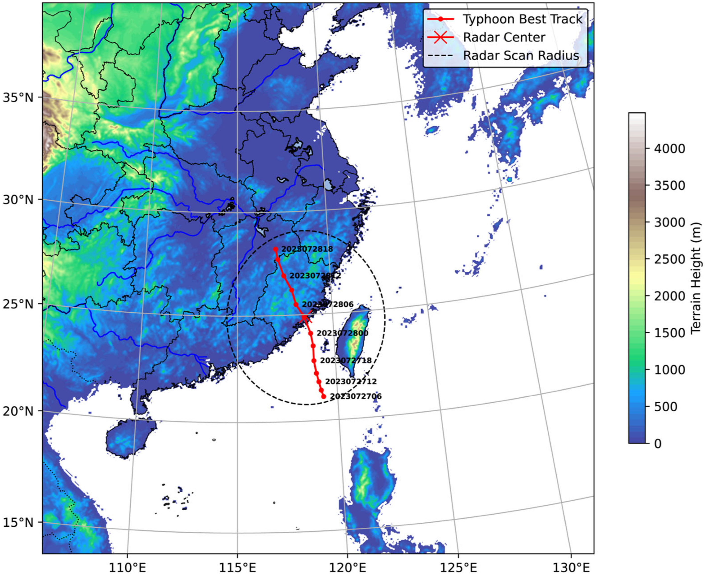
3.1.1. Typhoon Doksuri (2305)

Typhoon Doksuri (2023) is selected as the primary case in this study for detailed investigation of the impacts of radar data assimilation. It developed on 20 July 2023, beginning with a tropical depression in the western Pacific Ocean. It gradually strengthened and reached the severe tropical storm stage by 2100 UTC on 22 July, and later a typhoon at 0900 UTC on 23 July. On 24 July at 00:00 UTC, Doksuri intensified to a strong typhoon, and 12 h later it reached super typhoon strength, with a peak intensity of 62 m/s. As Doksuri continued its west-northwestward trajectory, it impacted the Philippines, making landfall at 1910 UTC on 25 July in the Babuyan Islands. The storm briefly weakened before regaining strength, and at 0155 UTC on 28 July Doksuri made landfall in Fujian Province, China, near Jinjiang City, as a strong typhoon, with maximum winds reaching 50 m/s (Category 15), causing extreme rainfall and widespread flooding. With a minimum pressure of 925 hPa and maximum gusts of 260 km/h, Doksuri brought devastating impacts across the Philippines and China. In the Philippines, Typhoon Doksuri was responsible for 30 fatalities and economic losses of approximately 15.32 billion PHP. In China, the typhoon caused 149.5 billion CNY in direct economic damage, with additional impacts from its residual low-pressure system, resulting in 154 fatalities. The total direct economic loss in China amounted to approximately 202.1 billion CNY. The main features of Typhoon Doksuri included a large, well-organized structure and persistent strong winds. Its slow movement over mainland China contributed to prolonged heavy rainfall, particularly in coastal areas. The storm’s intensity and track posed significant challenges for forecasting, making it an ideal case for testing numerical models and radar data assimilation techniques.

3.1.2. Typhoon Kompasu (2118)

Typhoon Kompasu (2021) is included as a supplementary case to provide a comparative perspective on the performance of the data assimilation schemes under a distinct typhoon scenario. Originating as a low-pressure area east of the Philippines, the system was classified as a tropical depression by the Japan Meteorological Agency (JMA) on 6 October 2021. On 8 October 2021, it intensified into a tropical storm and was internationally named Kompasu. The storm tracked westward, making an initial landfall in Cagayan, Philippines, on 11 October 2021. Kompasu continued into the South China Sea, intensifying further and reaching typhoon strength before its second landfall. On 13 October 2021, Typhoon Kompasu made landfall along the coast of Hainan Province, China, between Wenchang City and Lingshui City, with estimated wind speeds of 33–40 m/s. This made it the most powerful typhoon to strike Hainan in the preceding five years. The typhoon brought significant impacts, including widespread damage and dozens of fatalities, primarily in the Philippines, and also caused considerable economic losses in parts of China. After crossing Hainan, Kompasu weakened and eventually dissipated over Vietnam on 14 October 2021. The selection of Kompasu, a powerful typhoon affecting a region with available radar data (as indicated by the use of Haikou and Sanya radars in related studies), provides an opportunity to further assess the performance of the different momentum control variable schemes in radar data assimilation under a distinct typhoon event, complementing the analysis of Typhoon Doksuri.

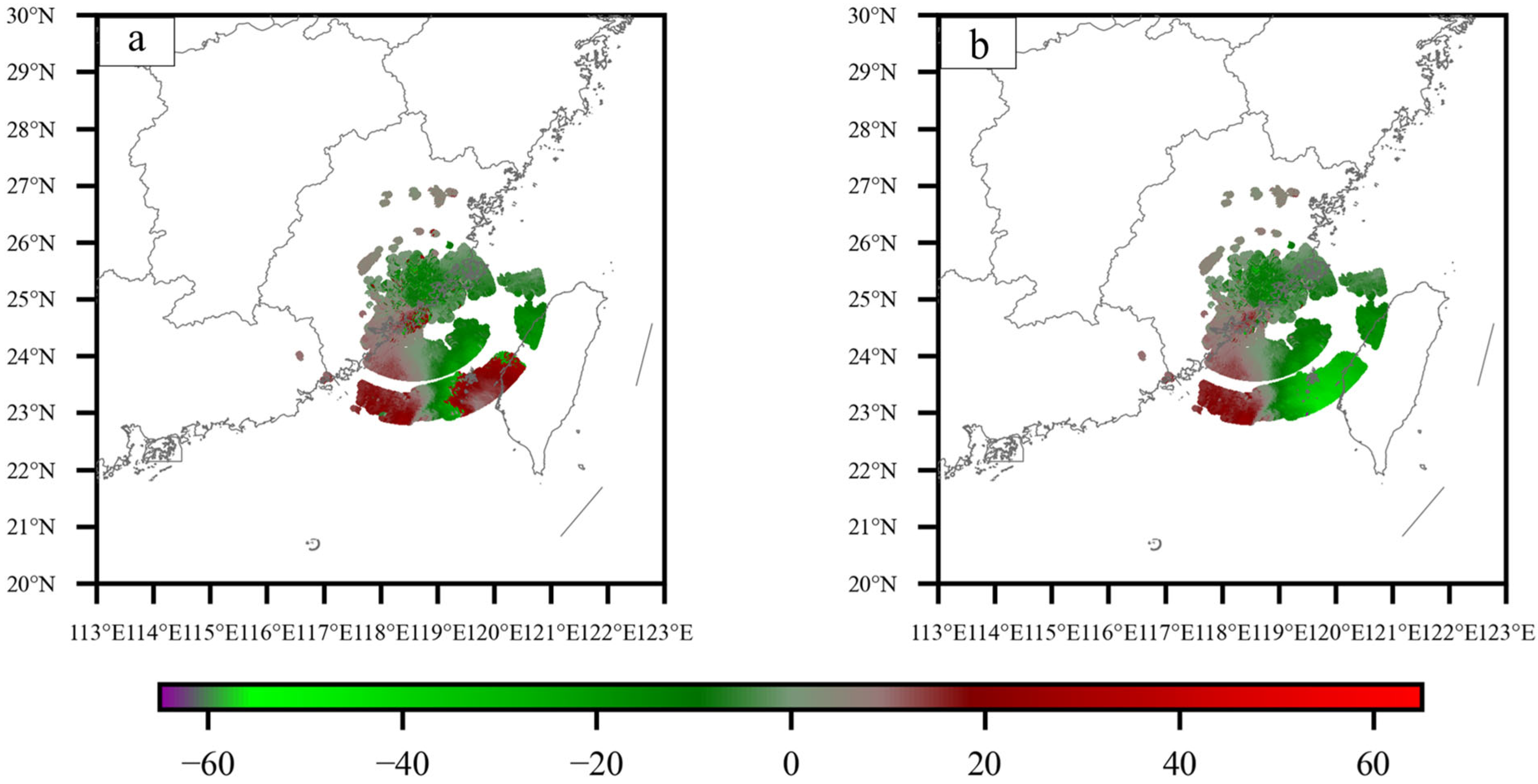
3.2. Radar Observation Processing

In this study, for the Typhoon Doksuri (2023) case, radar observations were obtained from an S-band dual-polarization Doppler weather radar situated in Quanzhou, Fujian Province (24.907° N, 118.587° E), with a maximum detection range of 460 km. The radar completed a full volume scan every 6 min, covering nine elevation angles: 0.5°, 1.5°, 2.4°, 3.3°, 4.3°, 6.0°, 9.9°, 14.6°, and 19.5°. For the Typhoon Kompasu (2021) case, radar data were sourced from two CINRAD systems in Hainan Province: the Haikou radar (CINRAD/SA; 19.996° N, 110.246° E, 118.0 m altitude) and the Sanya radar (CINRAD/SC; 18.228° N, 109.592° E, 443.0 m altitude). To ensure data reliability, the ${\mathrm{V}}_{\mathrm{r}}$ underwent rigorous quality control using the ARPS [37] and SOLO [38] systems. This process effectively removed erroneous signals caused by ground clutter, noise, and other artifacts. Following this, velocity de-aliasing procedures were applied to correct any phase wrapping errors. The detailed quality control procedures and the illustrative example in Figure 1 are presented for the Typhoon Doksuri case, with similar principles applied to the Typhoon Kompasu data. As Typhoon Doksuri approached the coastline, it moved fully into the radar’s observational domain, allowing for continuous and comprehensive monitoring. The observational error for the ${\mathrm{V}}_{\mathrm{r}}$ data was empirically set as 2 m/s in the present study, following Xiao et al. (2009) [39] and Shen et al. (2008) [8].

Figure 1 shows a comparison of the $V_r$ field prior to and following quality control at 1600 UTC on 27 July 2023, during the intensification phase of Typhoon Doksuri. In Figure 1a, the raw radar data show significant noise and incomplete velocity structures due to factors such as ground clutter and velocity aliasing. To address this, a modified four-dimensional dealiasing algorithm (FDDA) is used (Figure 1). The process begins by creating a wind profile using model background, rawinsonde, or wind profiler data. Background $V_r$ is calculated and compared with the radar data to identify aliased velocities. The velocities are then corrected using the Nyquist velocity, where the aliased velocity $V_a$ is adjusted as follows:

$$V_d=V_a+2N{V}_n,$$

(7)

where $N$ is an integer determined by the gate-to-gate shear threshold. Following dealiasing, the $V_r$ is interpolated into Cartesian coordinates and then spatially thinned, with a 10 km horizontal resolution and a 0.5 km vertical resolution. After the quality control process, Figure 1b shows that $V_r$ becomes significantly smoother and more coherent, forming a distinct cyclonic vortex structure. This improvement significantly enhances the accuracy of wind field. The maximum $V_r$ increases from approximately 25 m/s to over 50 m/s, which closely matches the observed values, demonstrating the effectiveness of the quality control process.

3.3. Model Setup and Experimental Design

In this study, all simulations were performed using version 4.1 of the Weather Research and Forecasting (WRF) model, coupled with version 4.6 of the WRF Data Assimilation (WRFDA) three-dimensional variational (3DVAR) system. Both typhoon cases were configured with a horizontal grid spacing of 5 km.

For the primary case, Typhoon Doksuri (2023), the model domain consisted of 601 × 601 horizontal grid points and 41 vertical levels, with the model top at 10 hPa. A relatively large domain was used to encompass both the tropical cyclone and its broader synoptic environment throughout the forecast period. This approach mirrors the setup in Shen et al. (2017) [40], where a large domain helped minimize potential lateral boundary effects in radar assimilation experiments. The domain was centered at 26.724° N, 119.353° E, covering the area of Fujian, China (see Figure 2). Initial and lateral boundary conditions were provided by Global Forecast System (GFS) data at 0.25° resolution and 6 h intervals, with the analysis fields for initialization and corresponding forecast fields for boundaries. The following physical parameterizations were applied: the Lin et al. microphysics scheme [41], the Kain–Fritsch cumulus scheme [42], the Yonsei University (YSU) planetary boundary layer scheme, the Rapid Radiative Transfer Model (RRTM) for longwave radiation [43], the Noah Land Surface Model, and the shortwave radiation scheme from the fifth-generation Pennsylvania State University–NCAR model [44]. This configuration is based on previous successful radar data assimilation studies of tropical cyclones, such as Shen et al. (2019) [31]. The simulation period for Doksuri was from 0600 UTC 27 July 2023 to 1800 UTC 28 July 2023. The best track data were provided by the China Meteorological Administration (CMA) and are shown in Figure 2.

A similar configuration was used for the supplementary case, Typhoon Kompasu (2021), with several specific adjustments. This simulation employed a 501 × 501 grid, 51 vertical levels, and a model top pressure of 50 hPa, centered at 20.3° N, 110.6° E. For Kompasu, the National Centers for Environmental Prediction (NCEP) Final Operational Global Analysis (FNL) data, with a 0.25° horizontal resolution and 6-hourly updates, were used to provide initial and lateral boundary conditions. The physical parameterization schemes were consistent with those used for Doksuri, except for the microphysics scheme: the WSM6 scheme was applied for Kompasu. The simulation period extended from 1200 UTC 12 October 2021 to 1800 UTC 13 October 2021, and the best track data were again obtained from the CMA.

For both typhoon cases (Doksuri and Kompasu), three experimental setups, summarized in

Table 1. Summary of experiments.

Number	Experiments	Assimilated Data
1	CTRL	None
2	3DVAR_a	radial velocity assimilation with $\psi -\chi$ control variables; radar reflectivity assimilation using the background-dependent retrieval method
3	3DVAR_b	radial velocity assimilation with $U-V$ control variables; radar reflectivity assimilation using the background-dependent retrieval method

, were designed. These include one control experiment (CTRL) without assimilation of data, one experiment with assimilation of data using $\psi -\chi$ control variables (3DVAR_a), and another experiment with data assimilation using $U-V$ control variables (3DVAR_b). Along with the control variables, both the 3DVAR_a and 3DVAR_b experiments also incorporated radar reflectivity assimilation using the background-dependent retrieval method. Figure 3 illustrates the experimental workflow for Typhoon Doksuri. In the DA experiments, radar data assimilation occurred at hourly intervals between 1200 UTC and 1800 UTC on 27 July. For Kompasu, the assimilation window was from 0000 UTC to 0600 UTC on 13 October 2021, also with hourly assimilation cycles (totaling seven cycles for each case). Since radar observations are concentrated in the early stage of these typhoons and primarily influence short-term forecasts due to their limited temporal and spatial extent, the forecast evaluation periods were chosen accordingly. For Typhoon Doksuri, the evaluation was extended to the first 24 h after the final assimilation cycle, as beyond this period the system significantly weakened and moved away from the primary radar coverage area, diminishing the direct impact of the assimilated radar data. For Typhoon Kompasu, the evaluation focused on the first 12 h post-assimilation, as the typhoon had moved offshore and away from the main observational domain relevant to this study beyond this timeframe.

4. Results: Typhoon Doksuri

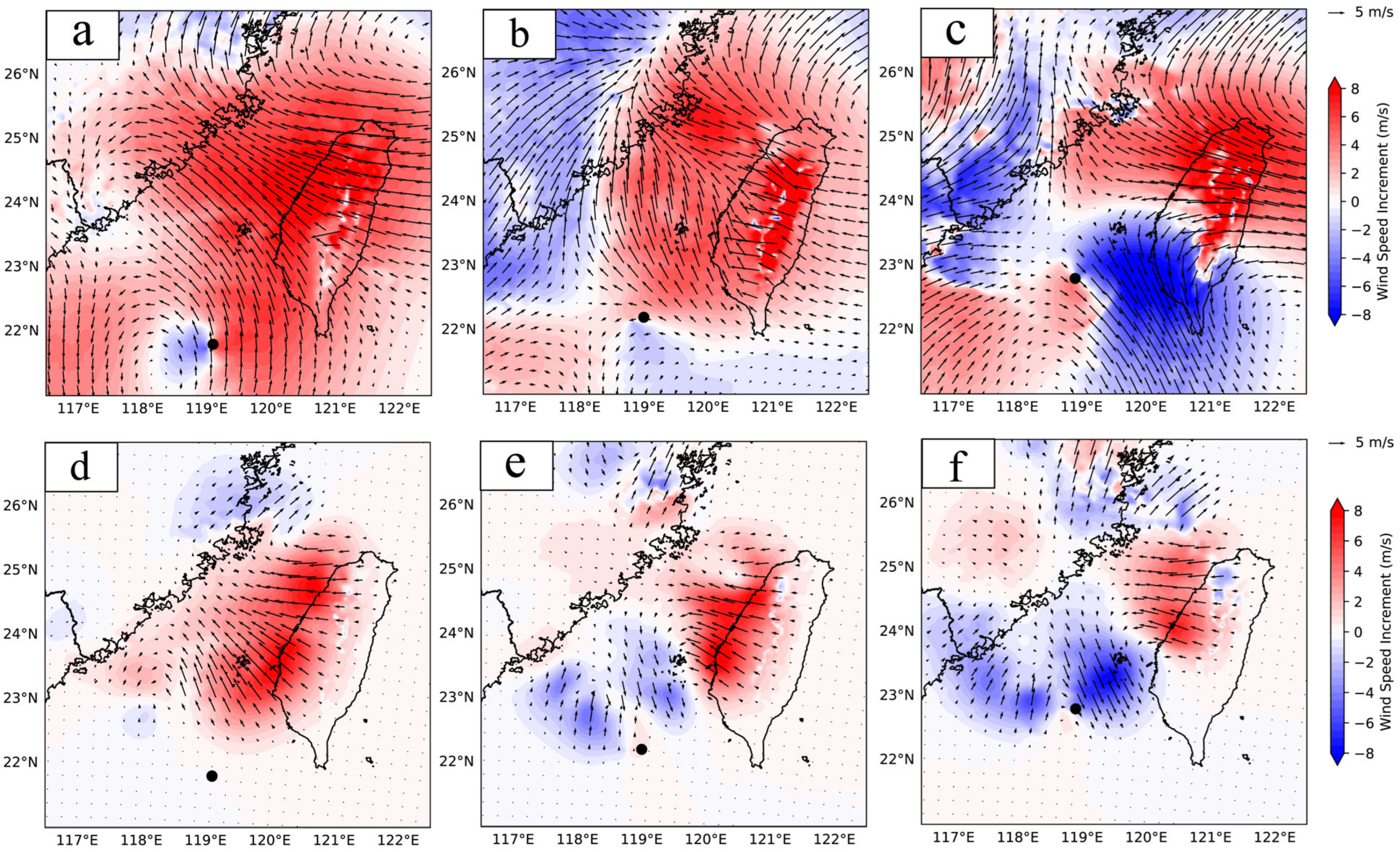
4.1. Assessment of Wind Increments

The experiment demonstrated that $V_r$ influences the wind field, with even more pronounced changes observed in the model’s dynamical field after seven assimilation cycles. Figure 4 presents the background and analyzed wind velocities and wind vectors at 700 hPa, observed at 1200 UTC on 27 July 2023.

In Figure 4a, the wind field is relatively weak, with less organized circulation. The typhoon center features a larger and less defined eye, with wind velocities below 20 m/s near the center. Wind vectors are more scattered, suggesting a broader and less intense system. In Figure 4b, the wind field strengthens, particularly in the eastern part of typhoon eye, where wind velocities exceed 40 m/s, with a more continuous wind field. This results in a more organized cyclonic structure with a tighter eye. The wind vectors in the northeastern quadrant show more concentrated and stronger winds compared to other areas of the storm. In Figure 4c, the wind field becomes more localized compared to Figure 4b. While the northeastern quadrant still exhibits strong winds, there is a noticeable reduction in wind speeds in the eastern part of the storm. The wind vectors remain organized, but the overall intensity in the northeastern quadrant decreases compared to Figure 4b. This suggests that, while the system remains relatively compact, the wind field’s intensity is more evenly distributed, and the storm’s core becomes slightly less concentrated.

Figure 5 illustrates the wind field analysis increments of 700 hPa corresponding to the initial assimilation cycle at 1200 UTC on 27 July 2023 for both 3DVAR_a and 3DVAR_b. In Figure 5a, a clear cyclonic wind field difference emerges near the typhoon center, where significant wind velocities variations are observed. This difference enhances typhoon intensity in the 3DVAR_a. An anticyclonic difference is also observed northeast of the typhoon center, which is in agreement with previous studies [45,46]. This imbalance is primarily caused by the use of $\psi -\chi$ control variables in 3DVAR_a, which represent the stream function and velocity potential. These variables are mathematically the integrated forms of the horizontal wind components $U$ and $V$, and their integral nature tends to preserve large-scale flow structures [47]. As a result, they can produce broad, smooth increments that lack localized dynamical features. This characteristic may introduce some non-physical errors into their analysis increment field [26], resulting in the presence of false cyclonic or anticyclonic characteristics in the analysis increment field. Such non-physical structures can distort the balance between wind and pressure fields, ultimately degrading the quality of the analysis and subsequent forecasts. The temporal evolution of assimilation increments was further examined by presenting wind fields at 700 hPa for three assimilation times—1200, 1500, and 1800 UTC on 27 July 2023—in both experiments. In Figure 5a–c, the increment patterns remain broad and diffuse across all cycles, with the anticyclonic anomaly northeast of the typhoon center persisting throughout. This indicates limited structural adjustment despite multiple assimilation updates. In contrast, Figure 5d–f exhibits progressively localized wind increments centered around the typhoon core. The evolution from broader to more compact increments suggests that the $U-V$ control variables allow for more efficient convergence and refinement of the analysis field over time. These results confirm that the $U-V$ formulation is more effective in supporting dynamic consistency and correcting forecast errors across successive assimilation steps.

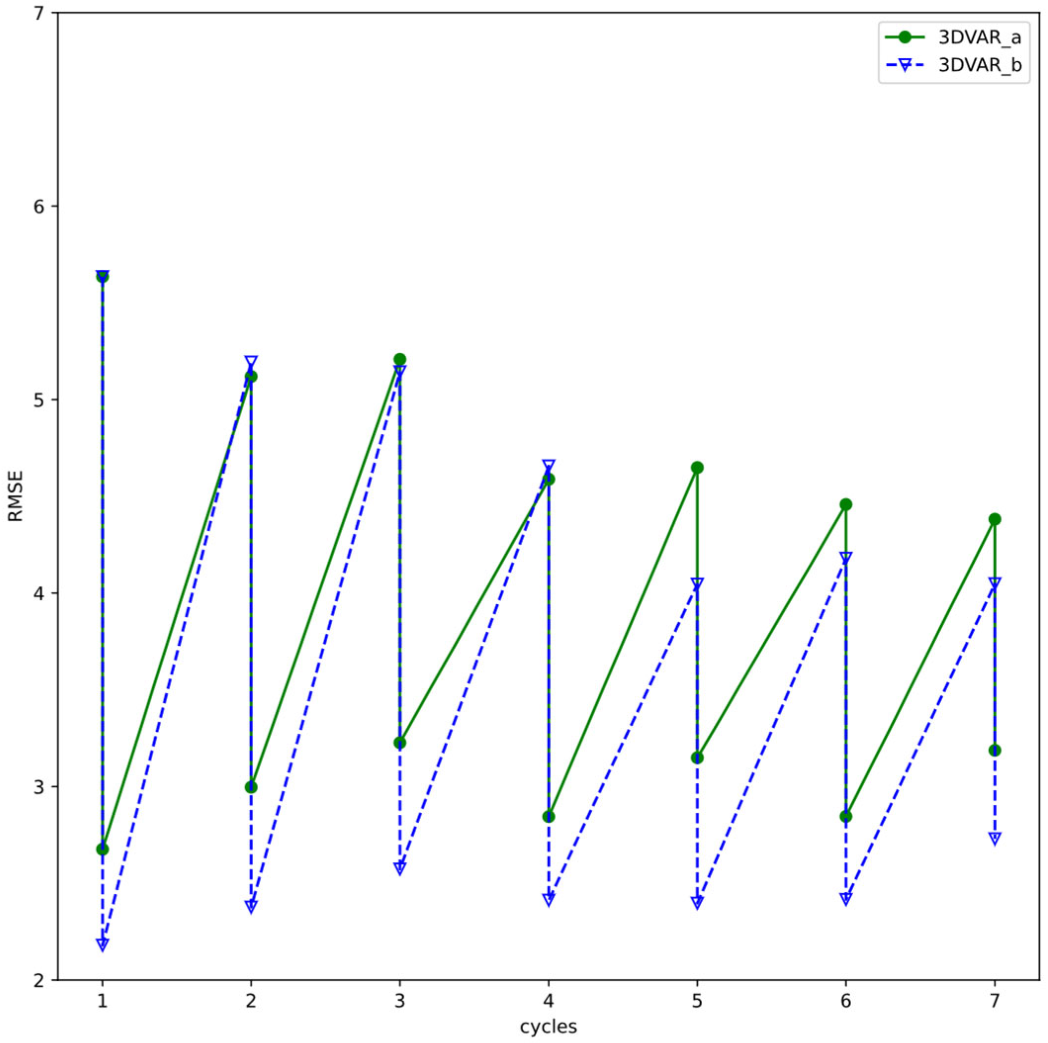
4.2. Statistics of Innovation for Vr in Data Assimilation Cycles

To quantitatively assess the assimilation effect quantitatively, the root-mean-square error (RMSE, strictly RMSD, as observations also contain error) is computed by comparing the analysis results and the observed radial velocities prior to and following each assimilation cycle. The corresponding results are shown in Figure 6. It can be seen that the RMSE of $V_r$ decreases following each DA cycle in every experiments. The largest decrease in RMSE occurs after the first analysis, as the raw background generally yields the largest observation increments. Throughout the DA cycles, RMSE values fluctuate between 2 and 6 m/s, as short-term forecasts derived from the analyses tend to increase the RMSE, whereas the DA analyses lead to a reduction. From Figure 6, it can be observed that the RMSE of 3DVAR_b consistently shows a larger decrease compared to 3DVAR_a. Following the first assimilation, the 3DVAR_b analysis exhibited a lower RMSE than 3DVAR_a. Additionally, the RMSE values for 3DVAR_b remained consistently lower than those for 3DVAR_a throughout the analysis. This suggests that the wind field in 3DVAR_b more closely approximated the observed conditions, indicating a more effective assimilation process. Ultimately, the RMSE of 3DVAR_a approaches 3.2 m/s, while the RMSE of 3DVAR_b is approximately 2.7 m/s.

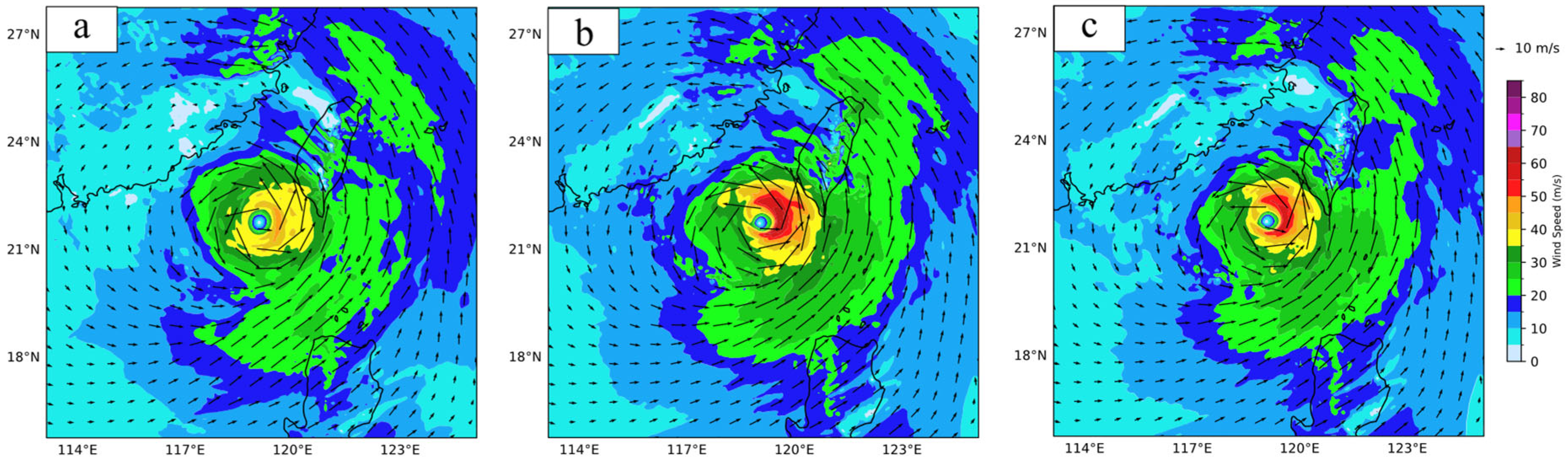
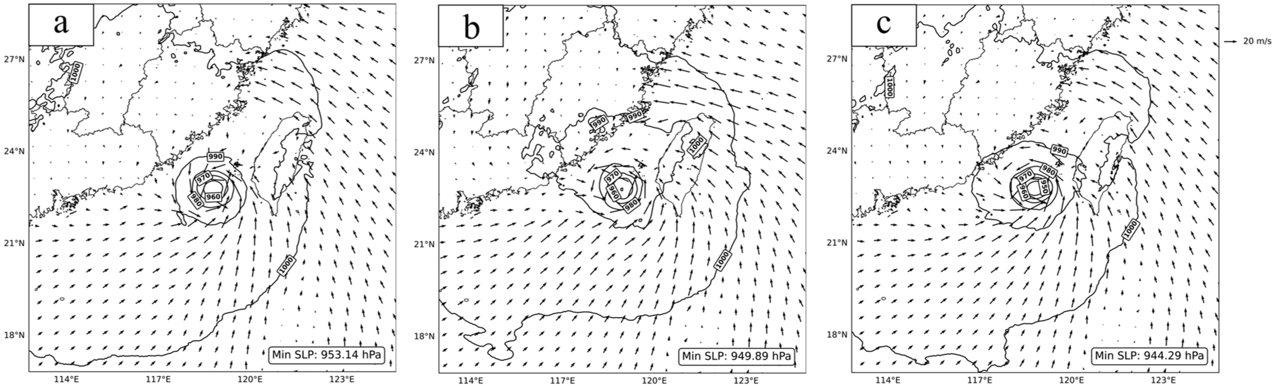
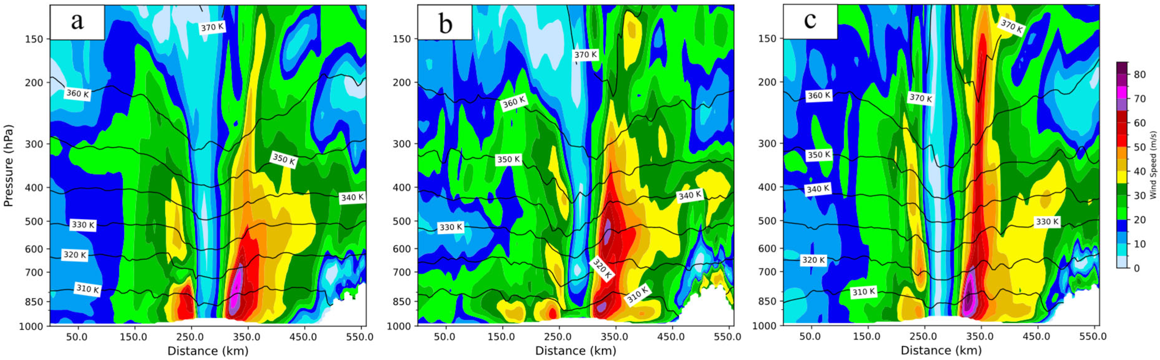
4.3. Typhoon Structure Examination

To assess typhoon intensity, sea-level pressure and surface wind speed are commonly used as key indicators. The final data assimilation cycle, occurring at 1800 UTC on 27 July 2023, is illustrated in Figure 7, which presents the analyzed mean sea-level pressure along with the corresponding surface wind vectors. Based on the CMA best track data, the minimum sea-level pressure was recorded at 930 hPa, with the peak surface wind velocity reaching 55 m/s. As shown in Figure 7a, the CTRL experiment notably underestimates typhoon strength, yielding a minimum sea-level pressure of 953 hPa and a maximum wind speed just over 50 m/s. In contrast, the 3DVAR_a experiment, as illustrated in Figure 7b, demonstrates closer agreement with the observations, capturing a deeper central pressure of 949.89 hPa and stronger surface winds exceeding 53 m/s. Figure 7c shows further improvement in 3DVAR_b, where the minimum sea-level pressure is 944.29 hPa, and the maximum wind velocity exceeds 57 m/s, which are close to the observed values. Moreover, the typhoon eye radius shrinks, the isobars become more tightly packed, and the core’s vortex is better defined. Overall, the 3DVAR_b experiment demonstrates more effective correction of the typhoon inner core, indicating that the assimilation of $V_r$ using $U-V$ control variables result in a more precise representation of the typhoon’s circulation structure.

To investigate the vertical structural evolution of the typhoon, Figure 8 illustrates the potential temperature and vertical cross-sections of horizontal wind speed. All experiments capture the characteristic asymmetry in the typhoon structure and successfully depict the vortex and eyewall features, which extend vertically from the surface up to around 100 hPa. In Figure 8a, corresponding to the CTRL experiment, the wind core is located near the 800 hPa level, with wind speeds gradually weakening above 700 hPa. The typhoon eye is distinctly defined, with horizontal wind speeds inside the eye remaining below 20 m/s. Compared to CTRL, 3DVAR_a (Figure 8b) substantially intensifies the wind field, with peak wind speeds exceeding 65 m/s. However, the maximum wind center is more dispersed and lacks a coherent core structure, likely due to imbalances between wind and pressure fields. This results in a more obscure typhoon center, and regions of wind speed below 20 m/s are absent at the lower levels. Figure 8c shows that 3DVAR_b not only enhances the wind field relative to CTRL but also modifies the flow pattern from a relatively flat distribution to a more vertically coherent, turbulent upward structure. The typhoon eye in 3DVAR_b is clearly resolved, with wind speeds consistently below 20 m/s along the vertical axis of the core. Among the three experiments, 3DVAR_b most closely aligns with the theoretical vertical structure of tropical cyclones and demonstrates a more realistic intensity. In contrast, 3DVAR_a distorts the vertical structure and introduces artificial convective features that degrade the integrity of the simulation.

Overall, both 3DVAR_a and 3DVAR_b improve the typhoon circulation and warm-core features. However, 3DVAR_b achieves better balance between wind speed and temperature fields, reduces anomalies, and provides a more consistent and physically realistic wind speed distribution, with enhanced high-altitude wind speeds demonstrating the advantages of using the $U-V$ control variable.

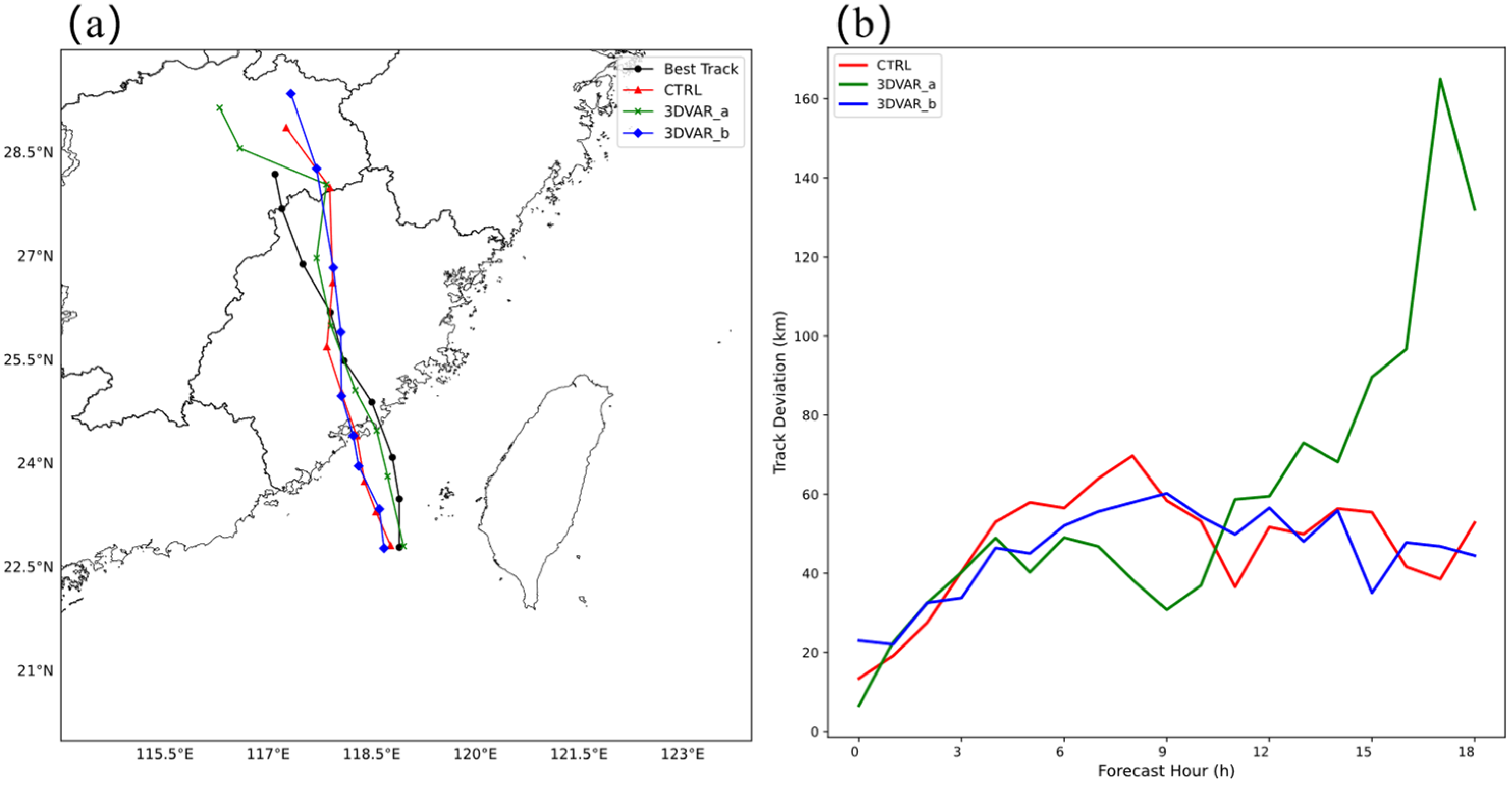
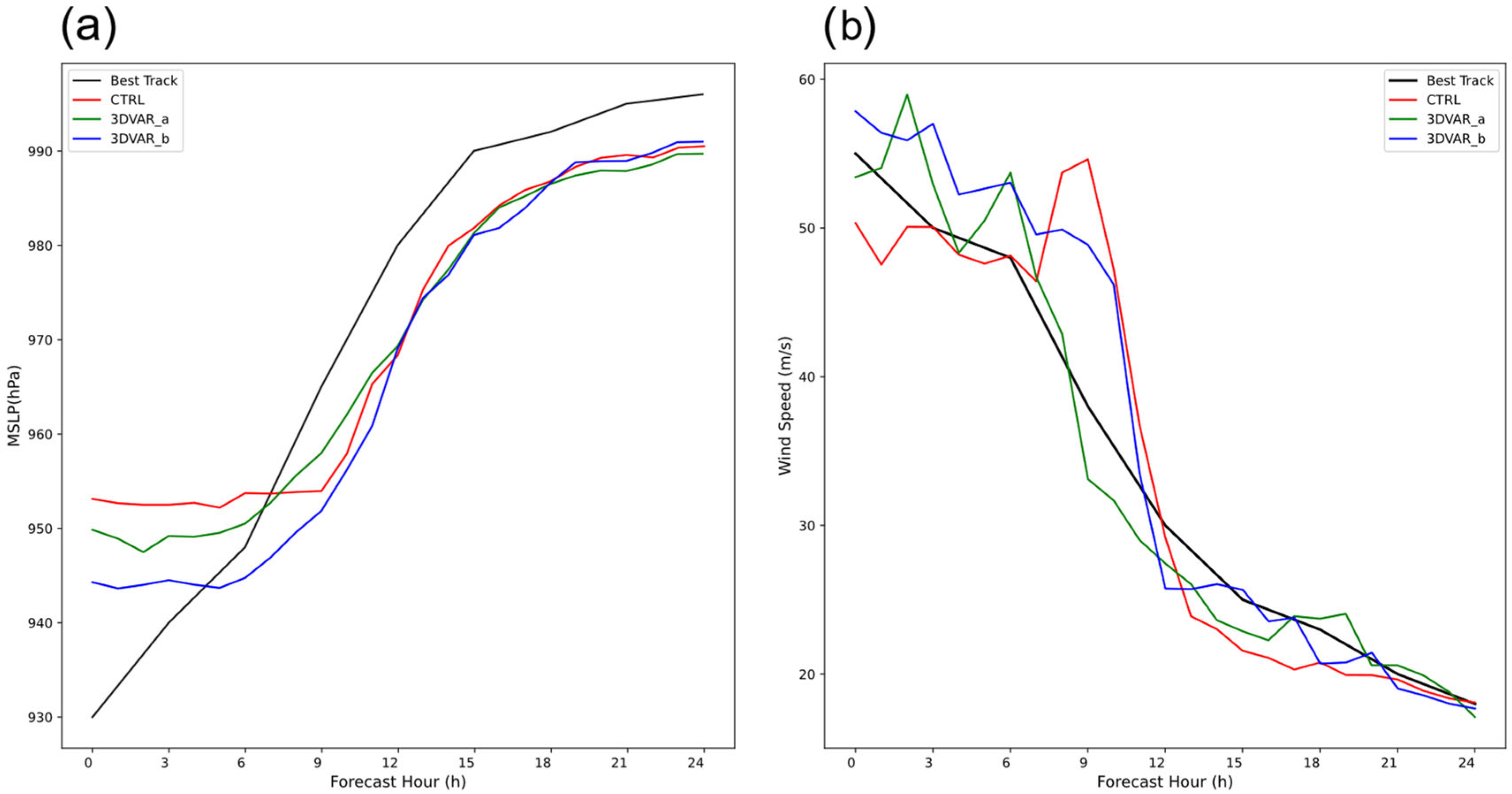
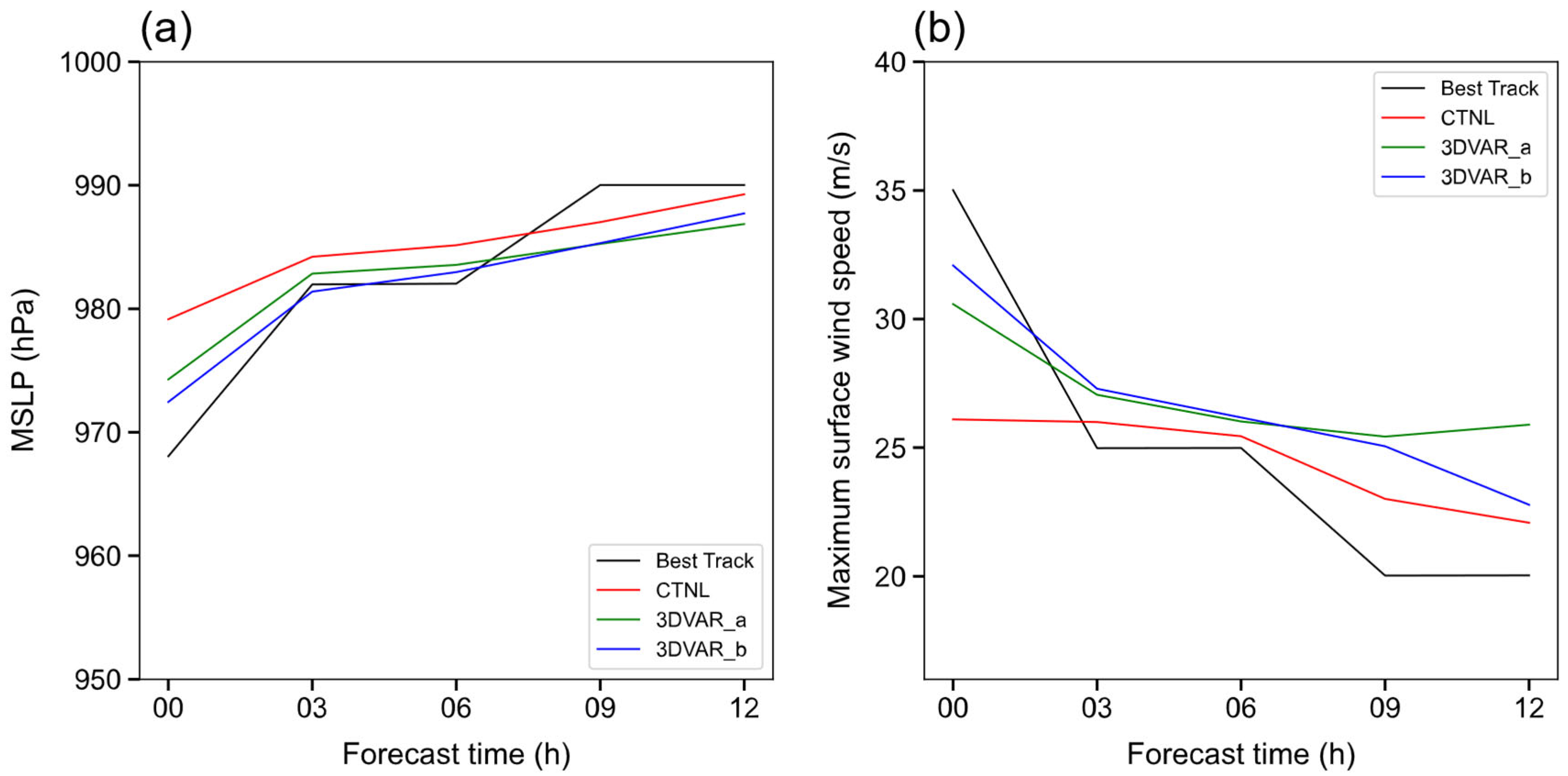
4.4. Forecast Track and Intensity Assessment

Figure 9a illustrates the forecast tracks for the three experiments over a 24 h period. Figure 9b presents the track deviations over an 18 h period. In Figure 9b, an evaluation of the track deviations reveals distinct performance characteristics for each assimilation experiment compared to the CTRL run, which, lacking data assimilation, generally exhibited substantial track deviations. The 3DVAR_a experiment, employing $\psi -\chi$ control variables, initially demonstrated the smallest track error. However, this early advantage was not sustained, and a significant drawback was the sharp increase in its track error during the later forecast hours, leading to the largest deviations among all experiments and an average 18 h deviation of 59.77 km. This late-stage deterioration may be linked to the known tendency of the $\psi -\chi$ formulation to introduce imbalances in certain mesoscale applications [26]. The 3DVAR_b experiment, using $U-V$ control variables, commenced with a larger initial track error than 3DVAR_a. However, its error profile remained relatively stable throughout the forecast period. Furthermore, the 3DVAR_b simulation avoided the significant late-stage error growth observed in the 3DVAR_a experiment. Consequently, 3DVAR_b achieved the lowest average track deviation of 45.65 km over the 18 h forecast period. This improved overall performance, reflected in the mean error and the stability against large deviations, suggests a beneficial impact from the $U-V$ control variables for this case.

The forecasted evolutions in minimum sea-level pressure (MSLP) and maximum surface wind (MSW) speed for Typhoon Doksuri from the three experiments (CTRL, 3DVAR_a, and 3DVAR_b) are compared with the CMA best track data in Figure 10. For MSLP, presented in Figure 10a, both 3DVAR_a and 3DVAR_b simulated a more intense initial typhoon than CTRL, with 3DVAR_b being relatively close to the observed MSLP of approximately 930 hPa. As the observed MSLP consistently rose, indicating typhoon weakening, 3DVAR_b’s forecast initially aligned more closely with the observations. Subsequently, while 3DVAR_a showed periods of better agreement, the MSLP forecasts from all three experiments became very similar in the later stages, specifically beyond approximately 13 h. During this period, the forecasted MSLP values were consistently lower than the observations, indicating that all simulations tended to portray a typhoon that weakened more slowly, or remained slightly more intense, than was actually observed. This common behavior suggests a potential shared model characteristic in representing the typhoon’s filling rate during its later phase.

The corresponding MSW forecasts are shown in Figure 10b. During the initial hour, the 3DVAR_b experiment simulated the highest initial MSW, slightly exceeding the observed 55 m/s, while CTRL significantly underestimated it. All simulations captured the overall MSW decrease. In the early hours, 3DVAR_b’s MSW forecast exhibited less variability than 3DVAR_a, though both initially simulated higher wind speeds than observed. In contrast, the CTRL simulation showed an uncharacteristic mid-forecast increase, deviating from the general weakening trend. In summary, for Typhoon Doksuri, the data assimilation experiments, especially 3DVAR_b, showed some improvements in representing initial typhoon intensity (MSLP and MSW) over CTRL. While challenges remained in accurately forecasting MSLP evolution in later stages and the MSW weakening rate, 3DVAR_b provided a more stable early MSW forecast and a more consistent overall weakening trend compared to CTRL’s erratic behavior. These aspects suggest potential benefits from the $U-V$ control variables, particularly for initial intensity and MSW trend. However, the complexities in forecasting this specific event’s intensity highlight the need for further evaluation of the schemes across multiple cases.

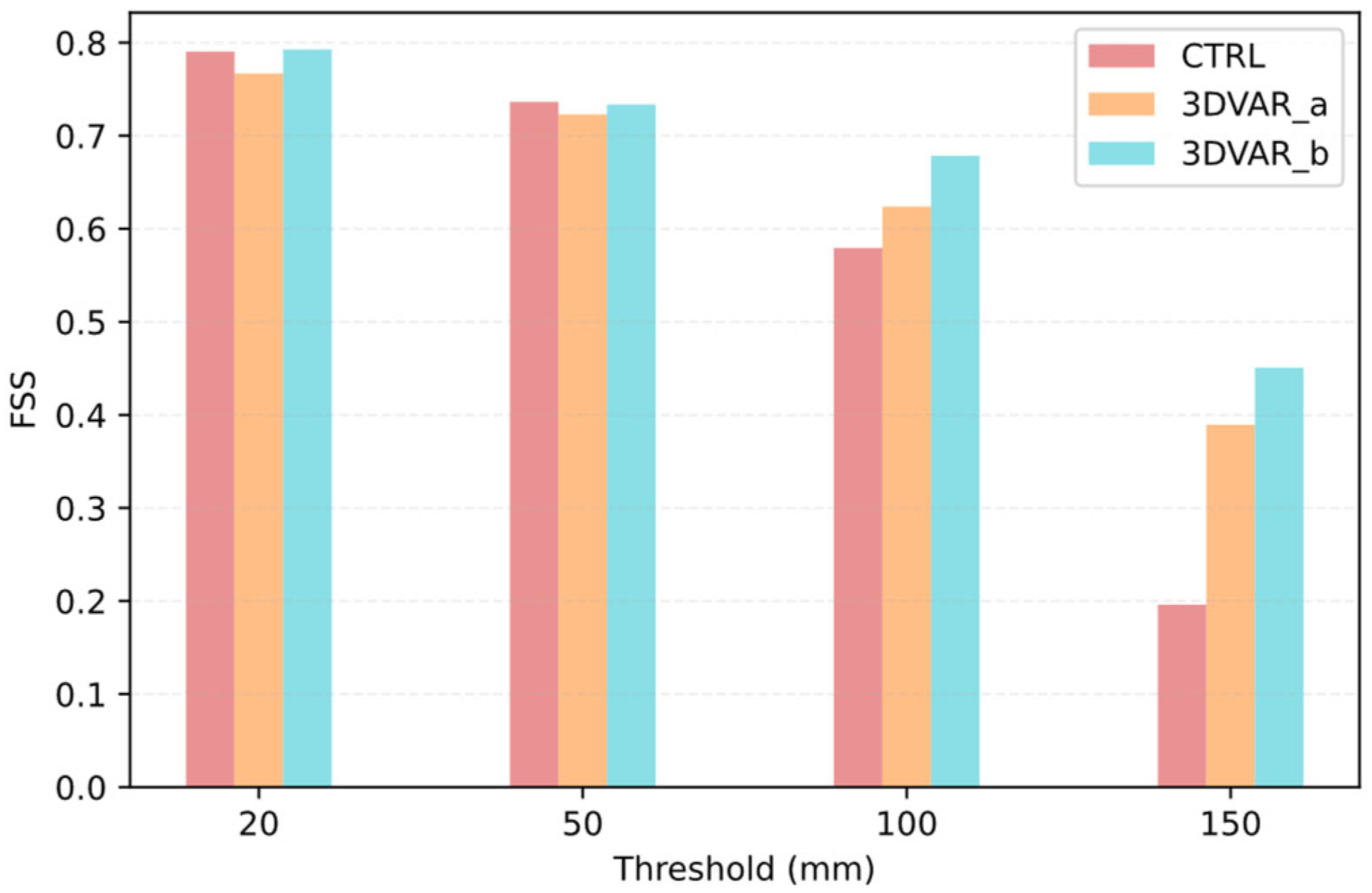
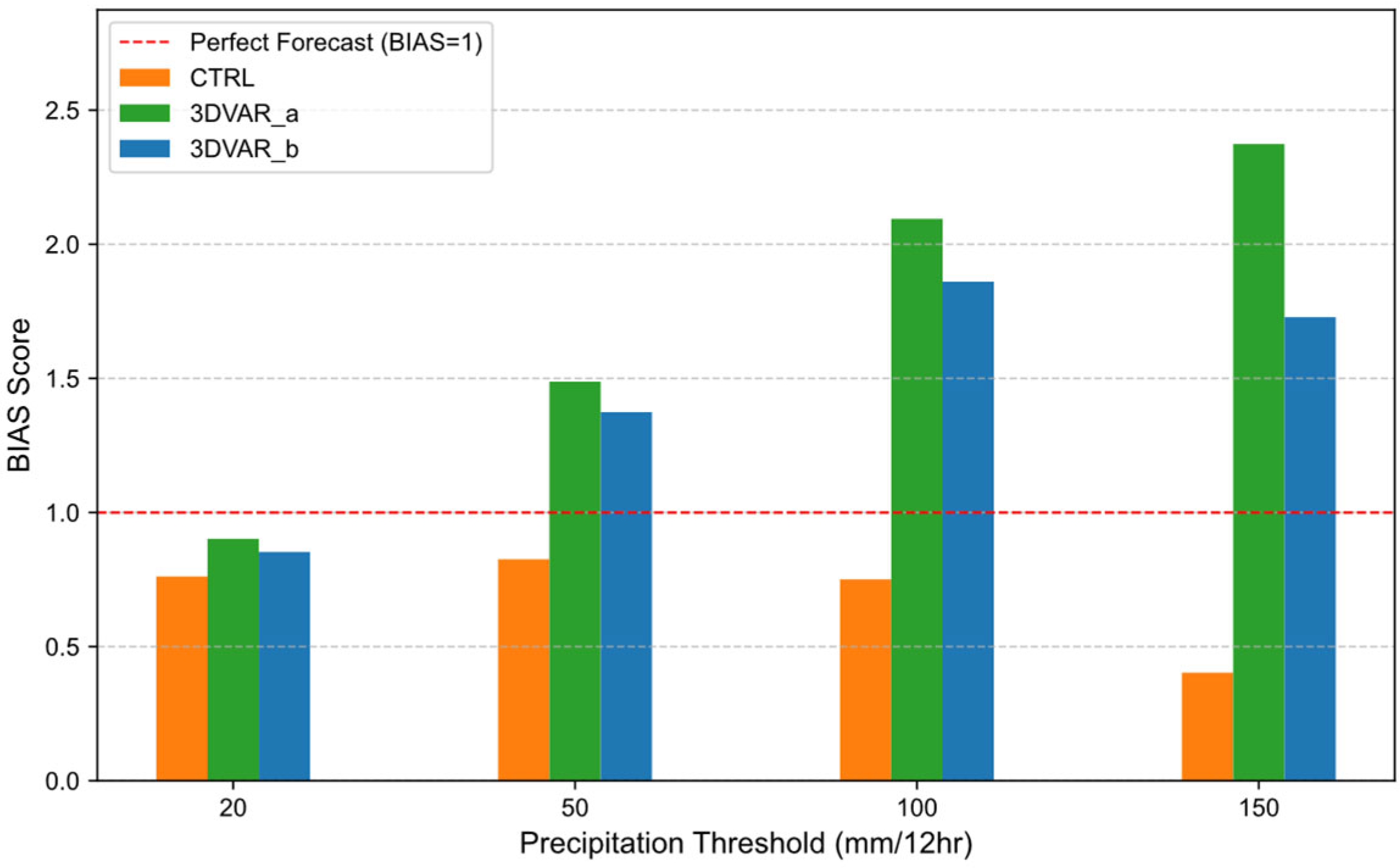
4.5. Precipitation Forecast Verification

The 12 h cumulative precipitation forecasts for Typhoon Doksuri, based on SYNOP station observations, are presented in Figure 11, showing distinct characteristics among the experiments. The observed significant precipitation was mainly concentrated along the southeastern coast of mainland China near the typhoon’s landfall point.

The CTRL experiment (Figure 11b) generally underestimated the heavy rainfall along the mainland coast, while overestimating precipitation over parts of Taiwan. It also exhibited some misplacement of precipitation centers and unrealistic remote rainfall bands.

Both data assimilation experiments, 3DVAR_a (Figure 11c) and 3DVAR_b (Figure 11d), produced substantially more intense and widespread precipitation compared to CTRL, more closely capturing the observed heavy rainfall areas along the mainland coast. However, the 3DVAR_a experiment, employing $\psi -\chi$ control variables, showed a tendency to significantly overestimate both the intensity and areal coverage of precipitation across multiple regions. In contrast, the 3DVAR_b experiment, using $U-V$ control variables, while also forecasting more intense precipitation than observed in some areas, provided a distribution and intensity that appeared more comparable to the SYNOP observations than 3DVAR_a. For instance, the extent of very heavy precipitation, such as areas receiving more than 300 mm, was considerably larger in 3DVAR_a than in both the observations and 3DVAR_b. Overall, while data assimilation generally improved the simulation of heavy rainfall areas compared to CTRL, the 3DVAR_b scheme offered a more realistic depiction of precipitation intensity and distribution than the 3DVAR_a scheme, despite a common tendency in the DA experiments to overestimate peak rainfall amounts relative to the SYNOP data.

Figure 12 illustrates the Fraction Skill Scores (FSSs) of 12 h cumulative precipitation for different thresholds. FSS provides a measure of precipitation forecast accuracy, with higher scores indicating better performance. This verification method, which compares forecasted rainfall with SYNOP station observations over different spatial scales, is a well-established approach in evaluating the skill of precipitation forecasts [48]. In this study, the FSS was calculated using a neighborhood radius of 15 km (corresponding to five grid points), which is a typical scale used in convection-permitting model evaluations [27,48]. Figure 13 presents the corresponding BIAS scores, which indicate overestimation (BIAS > 1) or underestimation (BIAS < 1) of precipitation frequency, providing additional context for the forecast skill assessment.

The FSS results (Figure 12) revealed varied levels of forecast skill depending on the precipitation threshold. At lower thresholds (e.g., 20 mm), CTRL and 3DVAR_b performed comparably to each other, and both were slightly better than 3DVAR_a. For moderate thresholds (e.g., 50 mm), CTRL exhibited the highest skill. However, as the threshold increased to 100 mm, and particularly to 150 mm (very heavy rainfall), the data assimilation experiments, especially 3DVAR_b, demonstrated a clear advantage in skill over CTRL, with 3DVAR_b achieving the highest FSS for these heavier precipitation categories.

The BIAS scores (Figure 13) provide important context. The CTRL experiment consistently underestimated the precipitation area across all thresholds (BIAS < 1), particularly for heavy rainfall. In contrast, both data assimilation experiments tended to overestimate the area of heavier precipitation (thresholds ≥ 50 mm). This overestimation tendency was most pronounced in 3DVAR_a, which exhibited a very high overestimation bias at the 100 mm and 150 mm thresholds. While 3DVAR_b also overestimated precipitation, its degree of overestimation was consistently less severe than that of 3DVAR_a, especially for heavier rainfall.

Considering both FSS and BIAS provides a more comprehensive assessment of forecast skill. The CTRL experiment, while exhibiting low bias, had low skill (FSS) in forecasting locations of heavy rainfall. Conversely, the 3DVAR_a experiment produced a higher FSS for heavy rain but at the cost of severe overestimation bias. The 3DVAR_b scheme offered the most balanced performance, achieving a high FSS for significant precipitation events (100 mm and 150 mm) while maintaining a considerably more constrained overestimation bias than 3DVAR_a. This suggests that the $U-V$ control variables provided a more balanced improvement to the heavy rainfall forecast for this case, enhancing skill in capturing the location of significant rainfall without the excessive overforecasting seen with the $\psi -\chi$ scheme (3DVAR_a).

5. Typhoon Kompasu Case Evaluation

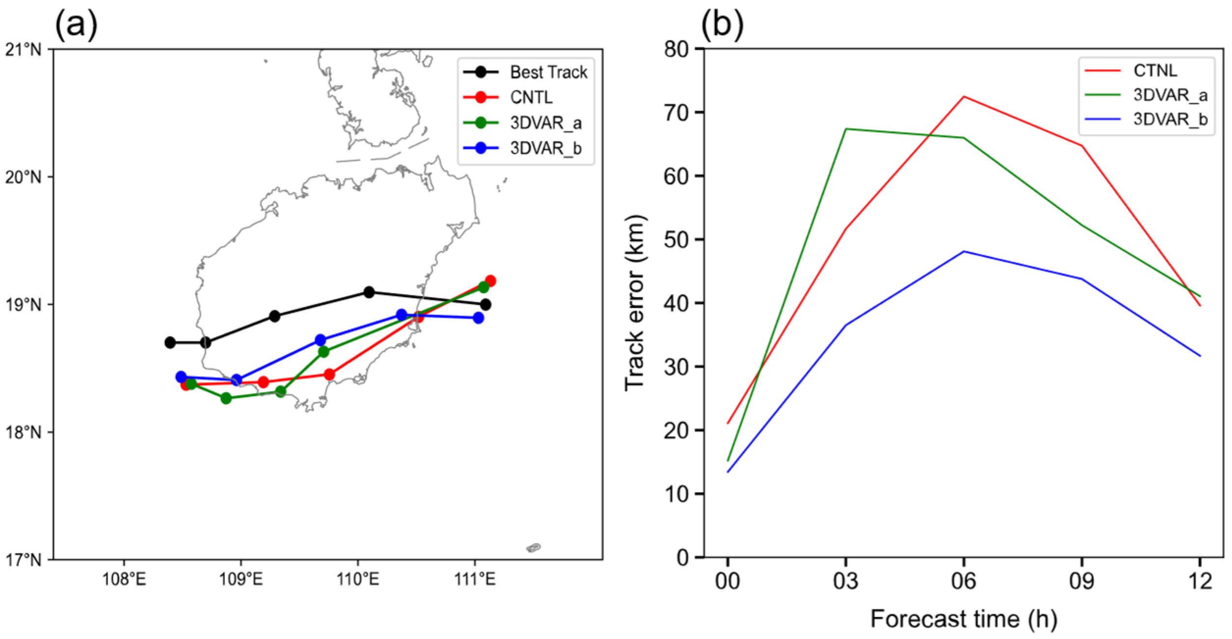
5.1. Track Forecast

The 12 h forecast tracks for Typhoon Kompasu, commencing from 0600 UTC on 13 October 2021, along with their respective errors, are presented in Figure 14. The 3DVAR_b experiment consistently yielded the most accurate track forecast throughout the 12 h period, demonstrating the smallest deviations from the CMA best track. Notably, the forecast from 3DVAR_b effectively captured the typhoon’s turning point, aligning closely with the observed trajectory. This improved performance, particularly during the 6 to 9 h forecast period where track errors in CTRL and 3DVAR_a were larger or showed inconsistent trends, can be attributed to the more physically coherent wind field analysis produced by the $U-V$ control variables. Such an analysis likely facilitated more rapid and appropriate adjustment towards a balanced state between the wind and mass fields in the typhoon’s vicinity, a factor that is critical for accurate track prediction. While the 3DVAR_an experiment showed some initial improvements over CTRL in terms of trend, its overall track error remained larger than 3DVAR_b. The superior track forecast from 3DVAR_b for Typhoon Kompasu reinforces the findings from the Typhoon Doksuri case and further underscores the benefits of the $U-V$ control variable scheme in radar data assimilation for TC prediction.

5.2. Intensity Forecast

The 12 h intensity forecasts for Typhoon Kompasu, in terms of minimum sea-level pressure (MSLP) and maximum surface wind speed (MSW), are compared against the CMA best track data in Figure 15. For MSLP, the 3DVAR_b experiment yielded the most accurate initial pressure and demonstrated the closest agreement with observations during the first 6 h of the forecast. While the CTRL experiment’s MSLP values were numerically closer to the underestimated observations in the later stages, this was largely attributed to its significantly weaker initial vortex. Regarding MSW, 3DVAR_b provided the best estimate of the initial wind speed. More importantly, the 3DVAR_b forecast maintained a consistent and physically plausible weakening trend throughout the 12 h period, aligning well with the observed evolution. This contrasts with the CTRL experiment, which substantially underestimated the initial MSW, and the 3DVAR_a experiment, which produced an unphysical increase in MSW in the final hours.

Overall, the assimilation using $U-V$ control variables (3DVAR_b) for Typhoon Kompasu showed clear benefit in initializing more realistic intensity and in forecasting a more consistent MSW trend. These results are consistent with the findings from the Typhoon Doksuri case and previous studies, such as Shen et al. [31] (2019), reinforcing the conclusions that the 3DVAR_b setup offers advantages for typhoon intensity prediction and that the observed improvements are not coincidental.

6. Conclusions and Discussion

This study investigated the impact of $\psi -\chi$ (3DVAR_a) and $U-V$ (3DVAR_b) momentum control variables within the WRFDA-3DVAR system, combined with a background-dependent radar reflectivity assimilation method, on forecasting Typhoons Doksuri (202305) and Kompasu (202118). Three experiments (CTRL, 3DVAR_a, 3DVAR_b) were conducted for each TC; Doksuri’s evaluation included track, intensity, precipitation, and vortex structure, while Kompasu’s analysis focused on track and intensity.

Radar data assimilation generally produced more realistic initial typhoon structures compared to CTRL for both cases. For Doksuri, wind increment analysis and innovation statistics showed that $U-V$ variables (3DVAR_b) yielded more localized and physically coherent wind field adjustments, more effectively assimilating radar data than the $\psi -\chi$ scheme (3DVAR_a), which sometimes produced broader, less realistic increments. Consequently, 3DVAR_b resulted in a better-defined vortex circulation and a more distinct warm-core structure in Doksuri.

Regarding Doksuri’s forecasts, 3DVAR_b achieved the lowest average track error and a more stable track forecast than 3DVAR_a, which exhibited significant late-stage error growth. For intensity, 3DVAR_b better represented the initial MSLP and MSW and a more consistent MSW weakening trend. Doksuri’s precipitation forecasts also indicated a more realistic depiction by 3DVAR_b than 3DVAR_a, especially for very heavy rainfall FSS scores.

The supplementary analysis of Typhoon Kompasu largely corroborated these benefits of $U-V$ control variables. For Kompasu, 3DVAR_b consistently produced smaller track errors, accurately captured the turning point, and showed advantages in initial intensity representation and MSW trend. The consistent performance of 3DVAR_b across two distinct typhoon events suggests that $U-V$ control variables generally offer a more robust and beneficial approach for radar data assimilation in TC forecasting than the $\psi -\chi$ scheme.

In conclusion, this study highlights that the selection of appropriate momentum control variables in radar data assimilation can enhance TC prediction. The $U-V$ control variable scheme, in particular, demonstrated relatively clear advantages in both the analyzed TC structure and subsequent forecasts. However, the complexities observed, especially in Doksuri’s intensity forecast, underscore that assimilation impact can be case-dependent. Therefore, while this dual-case study strengthens the findings, further research with more TC cases and varied assimilation strategies is necessary to confirm the general applicability and statistical robustness of these conclusions.

References

1. Pielke, R.A.; Gratz, J.; Landsea, C.W.; Collins, D.; Saunders, M.A.; Musulin, R. Normalized hurricane damage in the United States: 1900–2005. Nat. Hazards Rev. 2008, 9, 29–42. [Google Scholar] [CrossRef]
2. Xu, D.; Shen, F.; Min, J. Effect of background error tuning on assimilating radar radial velocity observations for the forecast of hurricane tracks and intensities. Meteorol. Appl. 2020, 27, e1820. [Google Scholar] [CrossRef]
3. Chen, J.; Xu, D.; Shu, A.; Song, L. The Impact of Radar Radial Velocity Data Assimilation Using WRF-3DVARSystem with Different Background Error Length Scales on the Forecast of Super Typhoon Lekima (2019). Remote Sens. 2023, 15, 2592. [Google Scholar] [CrossRef]
4. Li, Y.; Wang, X.; Xue, M. Assimilation of radar radial velocity data with the WRF hybrid ensemble–3DVAR system for the prediction of Hurricane Ike (2008). Mon. Weather Rev. 2012, 140, 3507–3524. [Google Scholar] [CrossRef]
5. Shen, F.; Song, L.; He, Z.; Xu, D.; Chen, J.; Huang, L. Impacts of adding hydrometeor control variables on the radar reflectivity data assimilation for the 6–8 August 2018 mesoscale convective system case. Atmos. Res. 2023, 295, 107012. [Google Scholar] [CrossRef]
6. Shen, F.; Song, L.; Min, J.; He, Z.; Shu, A.; Xu, D.; Chen, J. Impact of Assimilating Pseudo-Observations Derived from the “Z-RH” Relation on Analyses and Forecasts of a Strong Convection Case. Adv. Atmos. Sci. 2025, 42, 1010–1025. [Google Scholar] [CrossRef]
7. Shu, A.; Shen, F.; Li, H.; Min, J.; Luo, J.; Xu, D.; Chen, J. Impacts of assimilating polarimetric radar KDP observations with an ensemble Kalman filter on analyses and predictions of a rainstorm associated with Typhoon Hato (2017). Q. J. R. Meteorol. Soc. 2025, 151, e4943. [Google Scholar] [CrossRef]
8. Shen, F.; Min, J.; Xu, D. Assimilation of radar radial velocity data with the WRF Hybrid ETKF–3DVAR system for the prediction of Hurricane Ike (2008). Atmos. Res. 2016, 169, 127–138. [Google Scholar] [CrossRef]
9. Xu, D.; Chen, J.; Li, H.; Shen, F.; He, Z. The impact of radar radial velocity data assimilation using variational and EnKF systems on the forecast of Super Typhoon Hato (2017) with rapid intensification. Atmos. Res. 2025, 314, 107748. [Google Scholar] [CrossRef]
10. Carlin, J.T.; Ryzhkov, A.V.; Snyder, J.C.; Khain, A. Hydrometeor Mixing Ratio Retrievals for Storm-Scale Radar Data Assimilation: Utility of Current Relations and Potential Benefits of Polarimetry. Mon. Weather Rev. 2016, 144, 2981–3001. [Google Scholar] [CrossRef]
11. Carlin, J.T.; Gao, J.; Snyder, J.C.; Ryzhkov, A.V. Assimilation of ZDR columns for improving the spinup and forecast of convective storms in storm-scale models: Proof-of-concept experiments. Mon. Weather Rev. 2017, 145, 5033–5057. [Google Scholar] [CrossRef]
12. Caumont, O.; Ducrocq, V.; Wattrelot, É.; Jaubert, G.; Pradier-Vabre, S. 1D+3DVar assimilation of radar reflectivity data: A proof of concept. Tellus A 2010, 62, 173–187. [Google Scholar] [CrossRef]
13. Fierro, A.O.; Gao, J.; Ziegler, C.L.; Calhoun, K.M.; Mansell, E.R.; MacGorman, D.R. Assim-ilation of flash extent data in the variational framework at convection-allowing scales: Proof-of-concept and evaluation for the short-term forecast of the 24 May2011tornadooutbreak. Mon. Weather Rev. 2016, 144, 4373–4393. [Google Scholar] [CrossRef]
14. Fierro, A.O.; Wang, Y.; Gao, J.; Mansell, E.R. Variational assimilation of radar data and GLM lightning-derived water vapor for the short-term forecasts of high-impact convective events. Mon. Weather Rev. 2019, 147, 4045–4069. [Google Scholar] [CrossRef]
15. Zhang, F.; Weng, Y.; Sippel, J.A.; Meng, Z.; Bishop, C.H. Cloud-resolving hurricane initialization and prediction through assimilation of Doppler radar observations with an ensemble Kalman filter. Mon. Weather Rev. 2009, 137, 2105–2125. [Google Scholar] [CrossRef]
16. Snook, N.; Xue, M.; Jung, Y. Ensemble probabilistic forecasts of a tornadic mesoscale convective system from ensemble Kalman filter analyses using WSR-88D and CASA radar data. Mon. Weather Rev. 2012, 140, 2126–2146. [Google Scholar] [CrossRef]
17. Zhang, F.; Weng, Y.; Gamache, J.F.; Marks, F.D. Performance of convection-permitting hurricane initialization and prediction during 2008–2010 with ensemble data assimilation of inner-core airborne Doppler radar observations. Geophys. Res. Lett. 2011, 38, L15810. [Google Scholar] [CrossRef]
18. Snyder, C.; Zhang, F. Assimilation of Simulated Doppler Radar Observations with an Ensemble Kalman Filter. Mon. Weather Rev. 2003, 131, 1663–1677. [Google Scholar] [CrossRef]
19. Lei, L.; Whitaker, J.S.; Bishop, C. Improving assimilation of radiance observations by implementing model space localization in an ensemble Kalman filter. J. Adv. Model. Earth Syst. 2018, 10, 3221–3232. [Google Scholar] [CrossRef]
20. Bishop, C.H.; Hodyss, D. Flow-adaptive moderation of spurious ensemble correlations and its use in ensemble-based data assimilation. Q. J. R. Meteorol. Soc. 2007, 133, 2029–2044. [Google Scholar] [CrossRef]
21. Liu, J.; Bray, M.; Han, D. Exploring the effect of data assimilation by WRF-3DVar for numerical rainfall prediction with different types of storm events. Hydrol. Process. 2012, 27, 3627–3640. [Google Scholar] [CrossRef]
22. Wan, S.; Shen, F.; Chen, J.; Liu, L.; Dong, D.; He, Z. Evaluation of two momentum control variable schemes in radar data assimilation and their impact on the analysis and forecast of a snowfall case in central and eastern China. Atmosphere 2024, 15, 342. [Google Scholar] [CrossRef]
23. Sun, J.; Wang, H.; Tong, W.; Zhang, Y.; Lin, C.-Y.; Xu, D. Comparison of the impacts of momentum control variables on high-resolution variational data assimilation and precipitation forecasting. Mon. Weather Rev. 2016, 144, 149–169. [Google Scholar] [CrossRef]
24. Li, X.; Zeng, M.; Wang, Y.; Wang, W.; Wu, H.; Mei, H. Evaluation of two momentum control variable schemes and their impact on the var-iational assimilation of radar wind data: Case study of a squall line. Adv. Atmos. Sci. 2016, 33, 1143–1157. [Google Scholar] [CrossRef]
25. Sun, J.; Wang, H. Radar Data Assimilation with WRF 4D-Var. Part II: Comparison with 3D-Var for a Squall Line over the U.S. Great Plains. Mon. Weather Rev. 2013, 141, 2245–2264. [Google Scholar] [CrossRef]
26. Xie, Y.; MacDonald, A.E. Selection of Momentum Variables for a Three-Dimensional Variational Analysis. Pure Appl. Geophys. 2012, 169, 335–351. [Google Scholar] [CrossRef]
27. Chen, H.; Chen, Y.; Gao, J.; Sun, T.; Carlin, J.T. A radar reflectivity data assimilation method based on background-dependent hydrometeor retrieval: An observing system simulation experiment. Atmos. Res. 2021, 243, 105022. [Google Scholar] [CrossRef]
28. Shen, F.; Min, J.; Li, H.; Xu, D.; Shu, A.; Zhai, D.; Guo, Y.; Song, L. Applications of radar data assimilation with hydrometeor control variables within the WRFDA on the prediction of landfalling Hurricane IKE (2008). Atmosphere 2021, 12, 853. [Google Scholar] [CrossRef]
29. Barker, D.; Huang, X.Y.; Liu, Z.; Auligné, T.; Zhang, X.; Rugg, S.; Ajjaji, R.; Bourgeois, A.; Bray, J.; Chen, Y.; et al. The weather research and forecasting model’s community variational/ensemble data assimilation system: WRFDA. Bull. Am. Meteorol. Soc. 2012, 93, 831–843. [Google Scholar] [CrossRef]
30. Ide, K.; Courtier, P.; Ghil, M.; Lorenc, A.C. Unified notation for data assimilation: Operational sequential and variational. Meteorol. Soc. 1997, 75, 181–189. [Google Scholar] [CrossRef]
31. Shen, F.; Xu, D.; Min, J. Effect of momentum control variables on assimilating radar observations for the analysis and forecast for Typhoon Chanthu (2010). Atmos. Res. 2019, 230, 104622. [Google Scholar] [CrossRef]
32. Tong, M.; Xue, M. Ensemble Kalman Filter Assimilation of Doppler Radar Data with a Compressible Nonhydrostatic Model: OSS Experiments. Mon. Weather Rev. 2005, 133, 1789–1807. [Google Scholar] [CrossRef]
33. Smith, P.L.; Myers, C.G.; Orville, H.D. Radar Reflectivity Factor Calculations in Numerical Cloud Models Using Bulk Parameterization of Precipitation. J. Appl. Meteorol. 1975, 14, 1156–1165. [Google Scholar] [CrossRef]
34. Gilmore, M.S.; Straka, J.M.; Rasmussen, E.N. Precipitation and Evolution Sensitivity in Simulated Deep Convective Storms: Comparisons between Liquid-Only and Simple Ice and Liquid Phase Microphysics. Mon. Weather Rev. 2004, 132, 1897–1916. [Google Scholar] [CrossRef]
35. Gunn, K.L.S.; Marshall, J.S. The distribution with size of aggregate snowflakes. J. Meteorol. 1958, 15, 452–461. [Google Scholar] [CrossRef]
36. Posselt, D.J.; Bishop, C.H. Nonlinear data assimilation for clouds and precipitation using a gamma inverse-gamma ensemble filter. Q. J. R. Meteorol. Soc. 2018, 144, 2331–2349. [Google Scholar] [CrossRef]
37. Xue, M.; Wang, D.; Gao, J.; Brewster, K.; Droegemeier, K.K. The Advanced Regional Prediction System (ARPS), storm-scale numerical weather prediction and data assimilation. Meteorol. Atmos. Phys. 2003, 82, 139–170. [Google Scholar] [CrossRef]
38. Oye, R.; Mueller, C.; Smith, C. Software for radar data translation, visualization, editing and interpolation. In Proceedings of the 27th Conference on Radar Meteorology, Vail, CO, USA, 9–13 October 1995; AMS Committee: Boise, ID, USA; pp. 359–361. [Google Scholar]
39. Xiao, Q.; Zhang, X.; Davis, C.; Tuttle, J.; Holland, G.; Fitzpatrick, P.J. Experiments of hurricane initialization with airborne Doppler radar data for the Advanced Research Hurricane WRF (AHW) model. Mon. Weather Rev. 2009, 137, 2758–2777. [Google Scholar] [CrossRef]
40. Shen, F.; Xue, M.; Min, J. A comparison of limited-area 3DVAR and ETKF-En3DVAR data assimilation using radar observations at convective scale for the prediction of Typhoon Saomai (2006). Meteorol. Appl. 2017, 24, 628–641. [Google Scholar] [CrossRef]
41. Hong, S.-Y.; Dudhia, J.; Chen, S.-H. A revised approach to ice microphysical processes for the bulk parameterization of clouds and precipitation. Mon. Weather Rev. 2004, 132, 103–120. [Google Scholar] [CrossRef]
42. Kain, J.S.; Fritsch, J.M. A one-dimensional entraining/detraining plume model and its application in convective parameterization. J. Atmos. Sci. 1990, 47, 2784–2802. [Google Scholar] [CrossRef]
43. Mlawer, E.J.; Taubman, S.J.; Brown, P.D.; Iacono, M.J.; Clough, S.A. Radiative transfer for inhomogeneous atmospheres: RRTM, a validated correlated-k model for the longwave. J. Geophys. Res. 1997, 102, 16663–16682. [Google Scholar] [CrossRef]
44. Dudhia, J. Numerical study of convection observed during the winter monsoon experiment using a mesoscale, two-dimensional model. J. Atmos. Sci. 1989, 46, 3077–3107. [Google Scholar] [CrossRef]
45. Xiao, Q.; Sun, J. Multiple-radar data assimilation and short-range quantitative precipitation forecasting of a squall line observed during IHOP_2002. Mon. Weather Rev. 2007, 135, 3381–3404. [Google Scholar] [CrossRef]
46. Shen, F.; Xu, D.; Xue, M.; Min, J. A comparison between EDA-EnVar and ETKF-EnVar data assimilation techniques using radar observations at convective scales through a case study of Hurricane Ike (2008). Meteorol. Atmos. Phys. 2018, 130, 649–666. [Google Scholar] [CrossRef]
47. Shen, F.; Song, L.; Li, H.; He, Z.; Xu, D. Effects of different momentum control variables in radar data assimilation on the analysis and forecast of strong convective systems under the background of northeast cold vortex. Atmos. Res. 2022, 280, 106415. [Google Scholar] [CrossRef]
48. Roberts, N.M.; Lean, H.W. Scale-Selective Verification of rainfall accumulations from high-resolution forecasts of convective events. Mon. Weather Rev. 2008, 136, 78–97. [Google Scholar] [CrossRef]
Figure 1. Radial velocity comparison (shade, unit: ms−1) obtained from the Quanzhou radar (QZRD) at 1600 UTC on 27 July 2023: (a) V r before quality control and (b) V r after quality control.
Atmosphere 16 00797 g001
Figure 2. The domain of the WRF model, showing Typhoon Doksuri’s best track from 0600 UTC on 27 July to 1800 UTC on 28 July 2023. Obtained from the CMA Tropical Cyclone Data Center. The location of the radar center (QZRD) is indicated by an asterisk, and the radar scan radius is circled at 460 km. The terrain height is represented by shading (unit: m).
Atmosphere 16 00797 g002
Figure 3. The experimental flowchart for (a) the CTRL experiment and (b) the data assimilation experiments (3DVAR_a and 3DVAR_b).
Atmosphere 16 00797 g003
Figure 4. Wind vectors (arrow, reference vector = 10 ms−1) and wind velocities (shaded, unit: ms−1) at 700 hPa for (a) CTRL, (b) 3DVAR_a, and (c) 3DVAR_b at 1200 UTC on 27 July 2023.
Atmosphere 16 00797 g004
Figure 5. Analysis increments of wind vectors (arrows, reference vector = 5 m/s), wind speed (shaded, unit: ms−1) at 700 hPa, and the observed typhoon center (black dot) for different assimilation times. (ac) show the results from 3DVAR_a at 1200 UTC, 1500 UTC, and 1800 UTC on 27 July 2023, respectively. (df) show the results from 3DVAR_b at the same time points.
Atmosphere 16 00797 g005
Figure 6. Root mean square errors (RMSEs, unit: m/s) of V r (ms−1) for 3DVAR_a (green) and 3DVAR_b (blue) during cyclic assimilation.
Atmosphere 16 00797 g006
Figure 7. Surface wind vectors (arrow, reference vector = 20 m s−1) and analyzed mean sea-level pressure (black contour) for (a) CTRL, (b) 3DVAR_b3, and (c) 3DVAR_b at 1800 UTC on 27 July 2023.
Atmosphere 16 00797 g007
Figure 8. Potential temperatures (black contours, unit: K) and vertical profiles of the horizontal wind speed (shaded, unit: m/s) for (a) CTRL, (b) 3DVAR_a, and (c) 3DVAR_b at 1800 UTC on 27 July 2023.
Atmosphere 16 00797 g008
Figure 9. (a) Three forecast tracks from CTRL, 3DVAR_a, and 3DVAR_b and the CMA observations, spanning from 1800 UTC on 27 July to 1800 UTC on 28 July 2023; (b) track deviations (unit: km) of all the experiments relative to the CMA best track, from 1800 UTC on 27 July to 1200 UTC on 28 July 2023.
Atmosphere 16 00797 g009
Figure 10. (a) MSLP (unit: hPa) and (b) MSW (unit: ms−1) for CTRL, 3DVAR_a, and 3DVAR_b and the CMA observations from 1800 UTC 27 on July to 1800 UTC 28 on July 2023.
Atmosphere 16 00797 g010
Figure 11. Cumulative 12 h precipitation (units: mm) from 1800 UTC on 27 July 2023 to 0600 UTC on 28 July 2023: (a) SYNOP station observations, (b) CTRL, (c) 3DVAR_a, and (d) 3DVAR_b.
Atmosphere 16 00797 g011
Figure 12. Fractions Skill Scores (FSSs) for cumulative 12 h precipitation (mm) from 1800 UTC on 27 July 2023 to 0600 UTC on 28 July 2023, at thresholds of 20 mm, 50 mm, 100 mm, and 150 mm for the CTRL, 3DVAR_a, and 3DVAR_b experiments.
Atmosphere 16 00797 g012
Figure 13. BIAS scores for 12 h cumulative precipitation from the CTRL, 3DVAR_a, and 3DVAR_b experiments for Typhoon Doksuri at various thresholds (20 mm, 50 mm, 100 mm, and 150 mm per 12 h). The dashed red line indicates a perfect forecast (BIAS = 1).
Atmosphere 16 00797 g013
Figure 14. (a) Forecast tracks for Typhoon Kompasu from CTRL, 3DVAR_a, and 3DVAR_b experiments with the CMA best track, from 0600 UTC to 1800 UTC on 13 October 2021; (b) corresponding track errors (unit: km) relative to the CMA best track for the same 12 h period.
Atmosphere 16 00797 g014
Figure 15. (a) Minimum sea-level pressure (MSLP; unit: hPa) and (b) maximum surface wind (MSW; unit: m s−1) speed forecasts for Typhoon Kompasu from the CTRL, 3DVAR_a, and 3DVAR_b experiments and the CMA best track data, from 0600 UTC to 1800 UTC on 13 October 2021.
Atmosphere 16 00797 g015