Tracking Long-Term Ozone Pollution Dynamics in Chinese Cities with Meteorological and Emission Attribution

Abstract

Although China has achieved substantial reductions in particulate matter pollution, continually rising ground-level ozone now constitutes the primary challenge to further air-quality improvements. A systematic assessment of the long-term spatiotemporal behavior of ozone (O₃) and its links to meteorology and emissions is still lacking. Here, we develop a novel framework that couples Kolmogorov–Zurbenko (KZ) filtering with an optimized random forest (RF) regression model to examine daily maximum 8 h average ozone (O₃-8h) in 372 Chinese cities from 2013 to 2023. The approach quantitatively disentangles meteorological and emission contributions at the national scale, overcoming the limitations of traditional linear methods in capturing non-linear processes. Long-term components explain, in general, <40% of total O₃ variance. In eastern urban agglomerations, long-term meteorological factors—particularly temperature and surface ultraviolet radiation—account for up to 80% of the trend, whereas long-term emission contributions remain modest (≈5–6%), with pronounced signals in the Beijing–Tianjin–Hebei and Fenwei Plain regions. Empirical orthogonal function analysis further reveals distinct spatial patterns of emission influence: long-term O₃ trends in mega-cities such as Beijing, Tianjin, and Shanghai are driven mainly by local emissions (1.5–3% contribution), while key transport hubs including Xi’an, Tangshan, and Langfang are markedly affected by traffic-related emissions (>2%). These findings clarify the heterogeneous mechanisms governing O₃ formation across China and provide a scientific basis for designing and implementing the next phase of region-specific, joint prevention-and-control policies.

1. Introduction

Ground-level ozone (O₃) poses a serious threat to human health and terrestrial ecosystems [1]. In recent years, many countries—including China, the United States, Italy, and Japan—have promulgated ambient O₃ standards to safeguard air quality [2]. China has implemented phased air pollution control measures with marked success [3]. In 2013, the State Council issued the “Action Plan on Air Pollution Prevention and Control” [4]. It emphasized reducing the concentrations of particulate matter (PM10) and fine particulate matter (PM_2.5) [5]. In 2018, the State Council issued the “Three-Year Action Plan for Winning the Blue Sky Defense War,” which not only further reduced PM_2.5 concentrations but also promoted the establishment of clear emission reduction targets for sulfur dioxide and nitrogen oxides (NO_x) but also implemented volatile organic compound (VOC) management and control measures [6]. Since 2021, however, O₃ pollution has emerged as a new challenge: rapid population growth and economic activity have intensified O₃ exceedances in densely populated and economically vibrant metropolitan areas [7,8,9]. In 2023, 136 of China’s 339 prefecture-level cities failed to attain the national air quality standard; 79 of these exceeded the O₃ limit, and the national mean daily maximum 8 h average (O₃-8h) reached 124.6 μg/m³, representing a 4.0% increase from 2022 (Report on the State of the Environment in China, http://english.mee.gov.cn/Resources/Reports/soe/, last accessed 30 October 2024). Despite stringent precursor controls, the complexity of VOC sources, speciation, and reactivity continues to hamper effective O₃ abatement [10,11]. Importantly, O₃ and PM_2.5 are dynamically coupled [12]. On the one hand, O₃ is removed via heterogeneous uptake onto aerosol surfaces and by ozonolysis of unsaturated VOCs, a pathway that converts part of the oxidant into a secondary organic aerosol (SOA), thus acting as a sink for O₃ while simultaneously forming additional PM_2.5 [13]. On the other hand, the sharp decline in PM_2.5 since 2013 has weakened this uptake and reduced aerosol light scattering, allowing more actinic radiation to reach the surface and enhancing photochemical O₃ production [14]. These feedbacks help explain the frequently observed rise in O₃ alongside falling PM_2.5 concentrations [15] and underscore the need for a deeper, integrated understanding of the drivers of O₃ formation.

VOCs and NO_x are the key precursors to photochemical O₃ formation [16,17]. O₃ production and removal are also modulated, both directly and indirectly, by meteorological conditions [18,19]. Dang et al. found that in years with high O₃ pollution, high O₃ events were typically associated with elevated temperatures, which stimulated increased VOC emissions and enhanced the chemical formation of O₃ [20]. Wang et al. showed that adverse meteorological regimes characterized by high humidity and temperature can sustain pollution episodes, even under sharp emission reductions [21]. Solar radiation, particularly within the ultraviolet range, drives the photolysis of VOCs and NO_x, thereby influencing O₃ concentrations. Furthermore, wind speed plays a crucial role in the regional transport of pollutants; low wind speeds impede the dispersion of air pollutants, leading to their accumulation [22]. Quantifying the relative influence of meteorology and emissions is, therefore, critical for science-based O₃ control [23,24].

A growing body of work has attempted to disentangle these influences. While chemical transport models provide comprehensive insight, their high computational cost limits routine application. Consequently, statistical approaches, such as generalized additive models (GAMs) and multiple linear regression (MLR), have been widely employed to apportion the meteorological and emission contributions to pollutant variability [25,26]. The Kolmogorov–Zurbenko (KZ) filter, which separates variability on different temporal scales, has proved effective in assessing meteorological and emission impacts on PM_2.5 and O₃ [27,28]. Combining KZ with stepwise MLR, Mousavinezhad et al. [9] found that meteorology dominated O₃ variability in the Yangtze River Delta (YRD), Pearl River Delta (PRD), and South China coastal regions during 2015–2019, whereas precursor emissions controlled the increase in the Beijing–Tianjin–Hebei (BTH) region. Wu et al. combined the KZ filter with an MLR model, demonstrating that meteorological factors accounted for an average of 71.8% of the variability in O₃-8h concentrations in the Yangtze River Delta region [29]. Ding et al. (2023) used the time series decomposition method (STL) and random forest (RF) algorithm. Their results showed that the change in the Tianjin O₃ level was affected by meteorology for 13%, which was largely driven by the change in precursor emissions [30]. Nevertheless, most studies have been limited to single cities or regions, short time spans, or purely statistical frameworks, and a comprehensive national-scale comparison employing multi-scale decomposition, machine learning modeling, and spatial statistics is still lacking.

To fill this gap, we conduct a countrywide, long-term investigation of O₃ variation drivers with three specific objectives: (1) apply the KZ filter to decompose O₃-8h and meteorological observations for 372 prefecture-level cities (including autonomous regions and municipalities) from 2013 to 2023 and characterize their spatiotemporal patterns; (2) combine KZ filtering with an RF model to systematically quantify the long-term contributions of eight meteorological factors and emissions to the O₃-8h trend, thereby elucidating how the strength of meteorological forcing differs across the five major polluted regions (Figure 1); and (3) employ empirical orthogonal function (EOF) analysis to elucidate the spatiotemporal evolution of local long-term emissions and regional transport. The hybrid KZ–RF–EOF framework is adopted because RF lowers cross-validated RMSE relative to multiple linear regression while retaining interpretability, whereas EOF isolates transport-dominated versus locally dominated patterns. This comprehensive approach—combining multi-scale decomposition, non-linear machine learning regression, and spatial statistics—offers robust evidence for assessing meteorological modulation of O₃ control and provides a scientific basis for formulating region-specific mitigation strategies across China.

2. Materials and Methods

2.1. Data

The datasets utilized in this study are summarized in

Table 1. Data sources and calculation methods for O₃-8h and meteorological variables.

Variable	Source	Spatial Res.	Temporal Res.	Notes
O3-8h	TAP (1)	0.1° × 0.1°	Daily
T	ERA5 (2)	0.25° × 0.25°	Hourly
d2m	ERA5	0.25° × 0.25°	Hourly	For RH calc.
PS	ERA5	0.25° × 0.25°	Hourly
UVB	ERA5	0.25° × 0.25°	Hourly
u10, v10	ERA5	0.25° × 0.25°	Hourly	For WS/WD calc.
WS	Calculated (3)	N/A	Daily	Deriv. from u10 and v10
WD	Calculated	N/A	Daily
RH	Calculated	N/A	Daily	Deriv. from T and d2m

Notes: (1) Tracking Air Pollution in China (TAP) dataset. (2) ECMWF ERA5 Reanalysis dataset (original hourly data). (3) Calculated from ERA5 variables. Calc. = calculated; Deriv. = derived.

. Continuous O₃-8h concentration data from 2013 to 2023 were sourced from the Tracking Air Pollution in China (TAP) dataset (http://tapdata.org.cn/; accessed on 30 October 2024), with a daily temporal resolution and a spatial resolution of 0.1° × 0.1° [31,32]. Meteorological variables, including surface pressure (PS), 2 m temperature (T), 2 m dewpoint temperature (d2m), downward UV radiation at the surface (UVB), and 10 m wind components (u10 and v10), were derived from the Fifth Generation ECMWF Atmospheric Reanalysis (ERA5) dataset (https://cds.climate.copernicus.eu/; accessed on 30 October 2024). These data feature a daily temporal resolution and a spatial resolution of 0.25° × 0.25°.

Additional meteorological parameters were calculated based on the ERA5 dataset: wind speed (WS) and wind direction (WD) were derived from the u10 and v10 wind components, while relative humidity (RH) was calculated using the temperature and dewpoint temperature data. To obtain uniformly gridded, daily city-scale data, we intersected each 0.1°/0.25° raster layer with the shapefile polygons of the 372 prefecture-level cities and calculated the area-weighted mean of all grid cells whose centroids lay inside each boundary; the resulting averages provide one O₃-8h value—and matching meteorological variables—for every city on every day of the study period.

2.2. Separation of Temporal Scales Using the KZ Filter

In this study, the KZ filter was applied to decompose the O₃-8h time series into different temporal components by adjusting the window length and the number of iterations [33,34]. The pollutant concentrations were partitioned into short-term (X_ST), seasonal (X_SN), and long-term (X_LT) components. The short-term component primarily captures daily variations driven by rapid fluctuations in weather conditions and local emissions [35]. The seasonal component reflects periodic variations related to changes in solar radiation intensity, solar angle, and seasonal energy consumption patterns [27]. Meanwhile, the long-term component characterizes trends influenced by cumulative emissions and climate change [36]. The KZ_{(m, p)} notation indicates a moving average filter with a window length of m days applied iteratively p times. To effectively isolate each temporal component, the KZ_{(15, 5)} filter was utilized to remove short-term fluctuations, primarily white noise resulting from daily variability. Subsequently, the KZ_{(365, 3)} filter was employed to extract the long-term trends. This study adopts the KZ filter, widely used for air pollution time series analysis of PM_2.5 and O₃ [37,38,39,40], to separate the O₃-8h series into X_ST, X_SN, and X_LT components.

$$X(t)=X_{ST}(t)+X_{SN}(t)+X_{LT}(t)$$

(1)

X_BL(t) was obtained by applying the KZ_{(15, 5)} filter to X(t) and is defined as the sum of X_LT(t) and X_SN(t), effectively removing X_ST(t).

$$X_{BL}(t)=K{Z}_{(15,5)}[X(t)]=X(t)-X_{ST}(t)$$

(2)

The baseline component can be further decomposed into the daily climatological mean, $X_{BL}^{clm}$, defined as the average of X(t) over the study period, and the residual [39], $\epsilon \left(t\right)$, as follows:

$$X_{BL}(t)=X_{BL}^{clm}+\epsilon (t)$$

(3)

The final X_LT(t), X_ST(t), and X_SN(t) are calculated using the following formulas:

$$X_{LT}(t)=K{Z}_{(365,3)}[\epsilon (t)]$$

(4)

$$X_{ST}(t)=X(t)-X_{BL}(t)$$

(5)

$$X_{SN}(t)=X_{BL}(t)-X_{LT}(t)$$

(6)

2.3. Meteorological Adjustment Utilizing Time Series Decomposition

Assume the long-term O₃-8h trend comprises two main components. The first component is the long-term meteorological component, which is induced by changes in persistent meteorological conditions such as T, UVB, and RH. The second component is the meteorologically adjusted long-term emissions component, which reflects the O₃ variation trend predominantly driven by anthropogenic emission activities; the baseline component can be defined as follows:

$$X_{BL}(t)=X_{SN}(t)+X_{LT}^{met}(t)+X_{LT}^{emis}(t)$$

(7)

To quantify the influence of meteorological conditions on the long-term O₃ trend, we constructed city-specific RF regression models [41]. In this model, the baseline O₃-8h concentration (X_BL(t)) was used as the dependent variable, while the long-term baseline components of various meteorological variables (T, UVB, RH, PS, WS) served as independent variables to quantify the non-linear relationship between O₃ and meteorological factors. After chronological sorting, each city’s dataset was randomly partitioned into 70% for training, 15% for validation, and 15% for testing. The RF regression model is expressed as follows:

$$X_{BL}(t)=f\left(M_{BL,T},M_{BL,RH},\cdots ,M_{BL,i}\right)+{ϵ}_{BL}(t)$$

(8)

i denotes the baseline component of the meteorological variables, with i ∈ {T, UVB, RH, PS, WS}.

${\epsilon }_{BL}\left(t\right)$ is obtained by summing the long-term variation in emissions $X_{LT}^{emis}$ and the minor seasonal fluctuations that remain unexplained by the random forest regression model. The small seasonal variations removed by the KZ_(365,3) filter in conjunction with $X_{LT}^{met}$ are expressed as follows:

$$X_{LT}^{emis}(t)=K{Z}_{(365,3)}\left[{ϵ}_{BL}(t)\right]=X_{LT}(t)-X_{LT}^{met}(t)$$

(9)

2.4. Long-Term Trends of Local and Non-Local Emissions

EOF is a statistical method that decomposes a set of variables into linear combinations that capture the maximum total variance, and it can be applied across diverse fields, such as atmospheric science and oceanography [29,42,43,44]. In this work the long-term emission anomalies $X_{LT}^{emis}$ are arranged as a matrix with 372 city columns and time rows; the resulting correlation matrix is, therefore, 372 × 372 rather than 2 × 2. Solving its eigenvalue problem yields 372 EOF modes.

To make the subsequent attribution analysis tractable, these modes are regrouped by physical meaning rather than truncated. The leading, spatially coherent mode is interpreted as the transport-related component, whereas the residual field (obtained from the remaining modes) represents local variability.

$$X_{LT}^{emis}(t)=X_{LT}^{emis(L)}(t)+X_{LT}^{emis(T)}(t)$$

(10)

where superscripts L and T denote local and transport-related contributions, respectively. Equation (10) does not imply that only two EOFs exist; it simply partitions the full EOF expansion into two aggregated terms that are convenient for interpretation.

The corresponding principal component (PC) time series are dimensionless indicators of the temporal evolution of these two aggregated modes. For subsequent comparison with meteorological indices, the transport PC is linearly rescaled to the interval [−1, 1] as follows:

$$X_{LT}^{emis(T)}(t)=X_{LT}^{emis}(t)\times P{C}_t^{emis(T)}(t)$$

(11)

where ${PC}_t^{emis\left(T\right)}$ ∈ [−1, 1]. The combined EOF–PCA framework, therefore, provides a transparent means of separating city-scale and regional-scale influences on long-term emission variability, forming the basis for the attribution results presented in Section 3.

3. Results

3.1. Spatial and Seasonal Variability of O₃-8h Concentrations in China

A clear east–west gradient in the spatial distribution was observed, with consistently higher O₃-8h concentrations in eastern and central China than in the west throughout the three periods (Figure 2a–c). Compared with 2013–2017, the nationwide O₃-8h average concentration increased by roughly 8% in 2018–2020 and a further 3% in 2021–2023, indicating an overall upward trend rather than a net mitigation. During 2013–2017, elevated levels (>90 μg/m³) were mainly confined to the densely populated and economically developed North China Plain (NCP), YRD, and PRD. Between 2018 and 2020, concentrations intensified and hotspot values exceeded 105 μg/m³ in many NCP and YRD cities, reflecting persistent photochemical pollution driven by industrial activity, urbanization, and abundant precursor emissions [45]. In 2021–2023, although the eastern hotspots largely plateaued, O₃-8h concentrations continued to rise and spread across western and northern provinces (Figure 2c) so that areas exceeding 100 μg/m³ occupied a larger portion of the country than in previous intervals. This pattern underscores that, despite local improvements in some eastern cities, China as a whole still faces a widening and intensifying O₃ pollution challenge.

Seasonally, the highest O₃-8h concentrations were recorded during the summer months (Figure 3b), with peak levels frequently exceeding 120 μg/m³ in the NCP, YRD, and PRD. This is largely attributed to favorable meteorological conditions, including higher temperatures, intense UV radiation, and lower wind speeds, enhancing photochemical reactions. In spring (Figure 3a), concentrations remained relatively elevated, especially in the eastern regions, driven partly by increasing solar radiation and precursor emissions. In contrast, autumn (Figure 3c) exhibited moderate O₃ levels, with noticeable spatial variability. Eastern China still displayed relatively high concentrations (approximately 90–100 μg/m³), while other regions demonstrated lower O₃ values. Winter (Figure 3d) generally showed the lowest seasonal concentrations, predominantly below 80 μg/m³ nationwide, due to less favorable meteorological conditions (low temperature, weak radiation intensity) for O₃ formation [46].

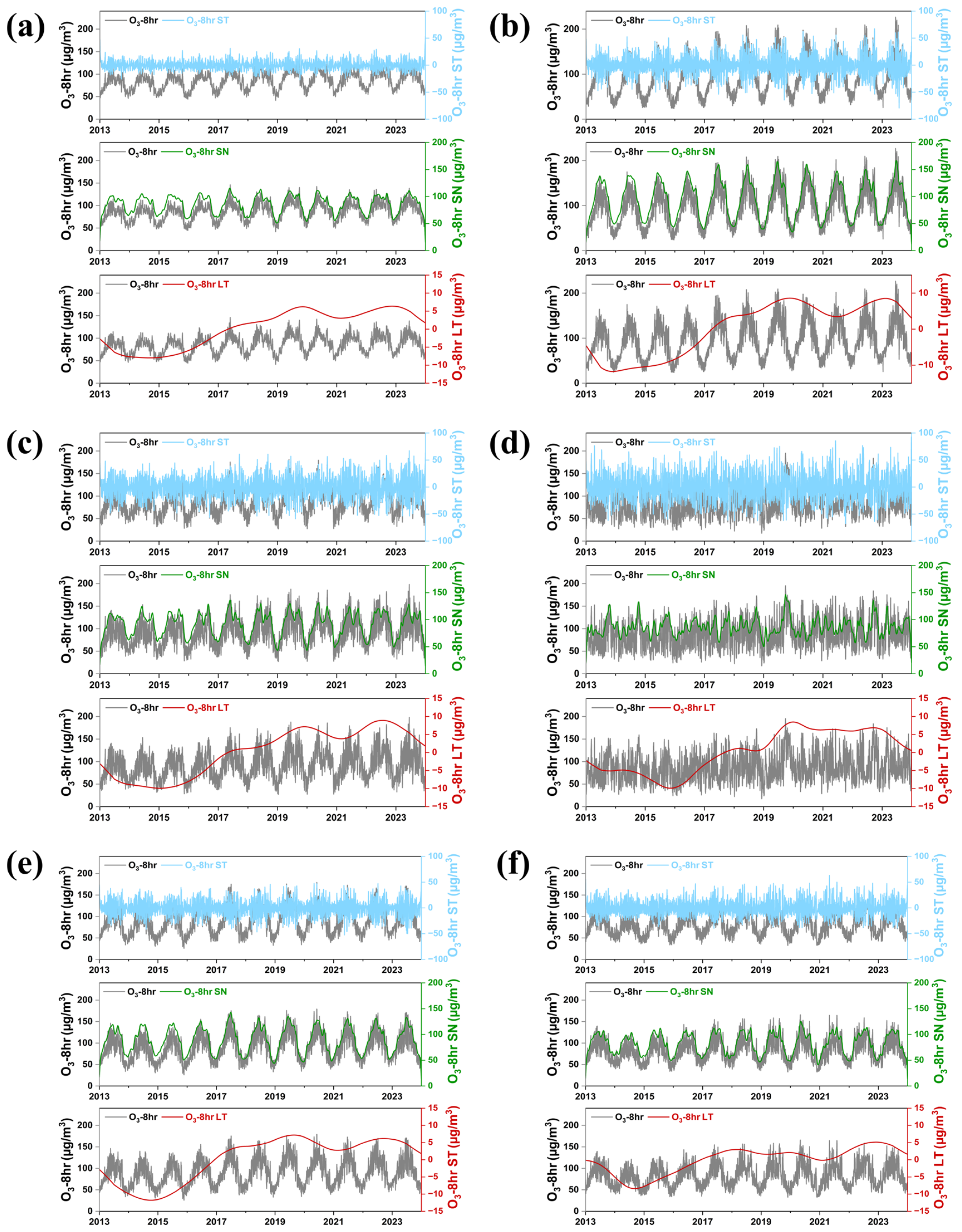
3.2. Temporal Decomposition of O₃-8h Concentrations

The contributions from X_ST, X_SN, and X_LT of O₃-8h concentrations exhibited pronounced spatial variations across China from 2013 to 2023 (Figure 4a–c). The X_ST term exerts its strongest influence along the southeastern seaboard—from the PRD through Fujian and up to parts of the lower Yangtze—where it accounts for roughly 50–60% of the total signal (Figure 4a). By contrast, the X_SN term peaks over western and northern China, where it contributes about 40–50% (Figure 4b). The X_LT component remains comparatively modest nationwide yet reaches 30–40% in the southwest (Yunnan–Guizhou and the Chengdu–Chongqing basin) and in the PRD (Figure 4c), highlighting the sustained impact of regional transport and long-term emission growth in these rapidly developing areas.

The temporal variations in the nationwide average O₃-8h concentrations, decomposed using the KZ filter into X_ST, X_SN, and X_LT components, further illustrate these distinctions (Figure 5a). The X_ST component shows burst-like excursions of 20 to 40 μg/m³. X_SN clearly demonstrates seasonal peaks in summer and lows in winter, driven predominantly by variations in temperature and solar radiation intensity [47]. The X_LT component, representing cumulative emissions and regional transport effects, displayed a steady increase after 2015, peaked around 2020, and, despite a slight decline after 2021, remained at elevated levels, underscoring persistent emission-related challenges.

Further decomposition for five major urban agglomerations—BTH, YRD, PRD, FWP, and CY—highlighted both common and distinctive features (Figure 5b–f). In BTH (Figure 5b), short-term pulses reach 60 μg/m³ during late spring dust storms, whereas the seasonal wave adds ~25 μg/m³ each July–August; the long-term curve climbs from 2015, plateaus in 2020, and then turns downward, mirroring NO_x control measures. The YRD (Figure 5c) exhibits the largest seasonal amplitude (30 μg/m³) and frequent sub-monthly oscillations in summer, suggesting strong marine air modulation; its X_LT rises rapidly until 2019 and then stabilizes. In the PRD (Figure 5d), the seasonal cycle dominates. X_SN peaks (>200 μg/m³) align with the onset of the southwest monsoon, while X_ST seldom exceeds 25 μg/m³, indicating relatively few extreme episodes. The inland FWP (Figure 5e) is characterized by pronounced X_ST surges—often >50 μg/m³—linked to stagnant, high-pressure conditions; a step-like increase in X_LT after 2017 coincides with the expansion of industrial activity in the FWP. CY (Figure 5f) shows the strongest interannual modulation within X_SN, driven by the East Asia summer monsoon’s variability; its X_LT turns sharply upward after 2019, implying a shift toward more persistent, emission-driven pollution.

Collectively, these detailed time series views demonstrate that X_ST is crucial in basins, such as the FWP and CY, whereas X_SN governs coastal agglomerations, like the YRD and PRD; X_LT continues to rise—or only recently plateaus—in all agglomerations, confirming that emission control efforts have yet to deliver sustained nationwide improvements.

3.3. Contribution of Meteorological Factors to O₃-8h

To quantitatively assess the influence of meteorological factors on O₃-8h concentrations, we first scaled each meteorological variable to a common 0–1 range before training the RF model. Specifically, for every factor (T, UVB, RH, PS, and WS), we identified its minimum and maximum values using the entire 2013–2023 record across all 372 cities and then expressed every daily value as a simple proportion of that overall range. In addition, we carried out a detailed analysis of the five most heavily polluted urban agglomerations; the city-level composition of each agglomeration is provided in Supplementary Figure S1. This whole-period min–max rescaling removes the effect of differing physical units while preserving the natural variability of each variable. The resulting normalized data were fed to the RF, which yielded the percentage contribution of each factor to the long-term O₃-8h baseline.

The spatial differences in the contributions of various meteorological factors to O₃-8h concentrations across China’s five typical urban agglomerations are illustrated in Figure 6a–e. T and UVB, as key factors directly influencing O₃ formation, are particularly prominent in the developed eastern regions. For instance, in the North China Plain—especially in Beijing and central Hebei—and in core cities of the YRD, such as Shanghai and Nanjing, the T contribution is significantly higher than in other regions, with maximum values exceeding 80%. This reflects the substantial enhancement of photochemical reactions by T in these key cities. Supplementary Figure S1 suggests that local topography may partly explain the heterogeneous influences of both T and UVB across different cities [48,49]. Meanwhile, the contribution of UVB exhibits an east, strong; west, weak pattern, with cities such as Beijing, Tianjin, and those in northern Hebei (e.g., Tangshan) showing particularly high contributions—exceeding 70%—which effectively promote the rapid generation of local O₃.

In contrast to T and UVB, the contributions of RH and WS display clear regional differences, closely related to the unique climatic and geographical conditions in different areas. In the PRD, particularly in cities like Guangzhou and Shenzhen, the contributions of humidity and wind speed reach over 70% and 60%, respectively, demonstrating the significant regulatory effect of moist marine monsoon conditions and strong regional transport on local O₃ concentrations, and this is relatively consistent with the findings of Xu et al. [50]. By contrast, in BTH and in cities such as Suzhou and Hangzhou in the YRD, the contribution of RH is lower, generally only 20–30%, and the wind speed contribution is also significantly weaker than in the PRD, suggesting that pollution accumulation in these areas is more dependent on the interplay between stagnant weather conditions and local emissions. Additionally, the contribution of atmospheric pressure is generally low across the five urban agglomerations—mostly maintaining at around 20–30%—although it is relatively prominent in parts of Xi’an (FWP) and Chongqing (CY).

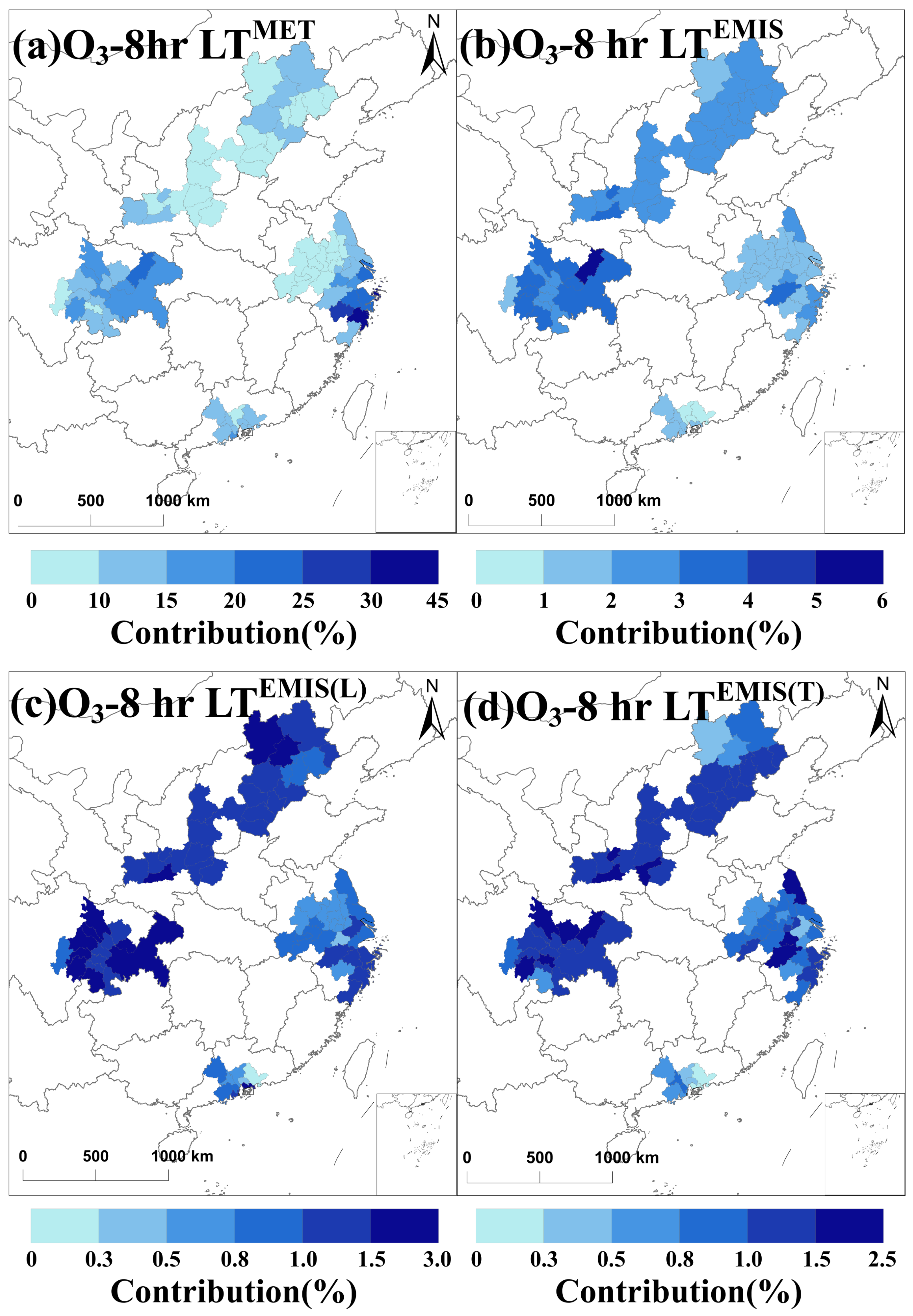
3.4. Quantitative Analysis of Meteorological and Emission Contributions to Long-Term O₃-8h Trends

The RF regression model was employed to quantitatively explore the relative contributions of meteorological and emission factors to the baseline O₃-8h concentrations (

Table 2. Performance metrics of RF regression models for baseline O₃-8h concentrations in five urban agglomerations.

Region	Validation R2	Validation MSE	Test R2	Test MSE
BTH	0.987	16.2	0.987	17.6
YRD	0.976	14.7	0.974	15.2
PRD	0.962	13.5	0.964	12.0
FWP	0.981	13.0	0.982	12.5
CY	0.984	7.1	0.984	6.8

). Model validation yielded high R² values (0.962–0.987), with relatively low mean squared errors (MSEs), demonstrating robust predictive performance across all five urban agglomerations. This high R² is largely attributed to the removal of short-term fluctuations in O₃-8h concentrations, as the regression was constructed using baseline components that capture only long-term variations. Specifically, the CY agglomerations achieved the highest validation and testing accuracy (validation R² = 0.984, test R² = 0.984), reflecting excellent reliability in this region. To quantify the relative contributions of meteorological conditions and emissions to long-term O₃-8h variations, this analysis assumes that the contributions of short-term meteorology, short-term emissions, seasonal meteorology, seasonal emissions, long-term meteorology, and long-term emissions are separately quantified and normalized, with their combined contributions summing to unity (100%). This section specifically focuses on evaluating and interpreting the long-term components of meteorology (O₃-8h LT^MET) and emission factors (O₃-8h LT^EMIS), emphasizing their regional disparities and relative significance in driving observed O₃ trends.

The contributions of meteorological factors and emissions to long-term O₃-8h trends showed pronounced regional differences (Figure 7). In Figure 7, each point represents an individual city, and the color of the point identifies the urban agglomeration to which that city belongs. Among the five urban agglomerations, the YRD exhibited the widest range of meteorological contributions, varying from approximately 10% to over 40%, indicating a high sensitivity of O₃ pollution to meteorological variations. Conversely, emission contributions were relatively higher and more concentrated in the FWP and CY agglomerations, typically ranging between 2% and 4%. A least-squares fit across all cities yields the relationship (y = 0.04x + 1.81); however, the associated coefficient of determination is only R² = 0.09, signifying a very weak linear link between meteorological and emission contributions rather than a moderate one. The low R² reflects the marked heterogeneity of both climate regimes and emission profiles among the different urban agglomerations—eastern coastal cities (e.g., YRD) are strongly modulated by meteorology, whereas emission-driven influences dominate in the PRD and FWP—so the combined national dataset does not conform to a single, tight linear trend. These regional disparities diminished the total correlation when assessed at the national scale.

EOF decomposition further clarified the spatial distribution of driving factors affecting long-term O₃-8h trends (Figure 8). O₃-8h LT^MET significantly influenced northern regions (Figure 8a), including the BTH area and parts of the YRD, exceeding 25% contribution and reflecting the strong dependence of O₃ formation on temperature and solar radiation. In contrast, O₃-8h LT^EMIS exhibited relatively uniform spatial contributions (Figure 8b), peaking around 4–5% in urbanized agglomerations, such as the PRD and FWP. To further distinguish between local and non-local (transport-related) emission impacts, emission contributions were decomposed into local emissions (O₃-8h LT^EMIS(L)) and transport-related emissions (O₃-8h LT^EMIS(T)) (Figure 8c,d). Local emissions dominated urban agglomerations, particularly in BTH and YRD, reflecting intensive anthropogenic activities and stationary emission sources. Conversely, transport-related emissions played a more prominent role in peripheral cities and regions near administrative boundaries, highlighting the importance of inter-city pollutant transport processes.

When specifically normalizing emission-related impacts to isolate local versus transport contributions (Figure 9), notable distinctions emerged among agglomerations. Transport emissions dominated in the PRD (59%) and CY (55%), underlining the influence of cross-regional pollutant transport. In contrast, local emissions were particularly significant in the YRD and FWP (both 53%), emphasizing local source controls as critical for mitigating long-term O₃-8h pollution in these densely populated and industrially intensive regions.

4. Discussion

4.1. Regional Variations in the Spatiotemporal Distribution of O₃-8h in China

The observed east–west gradient in O₃-8h concentrations, with eastern regions (NCP, YRD, PRD) consistently exceeding 90 μg/m³ compared to lower levels in western areas, reflects the interplay of economic activity, emission profiles, and regional meteorology. The nationwide increase of 8% in 2018–2020 and an additional 3% in 2021–2023 indicates that existing emission controls have not sufficiently offset the combined effects of industrial expansion and favorable photochemical conditions [51]. The westward expansion of high-concentration zones (>100 μg/m³) in 2021–2023, extending to western and northern provinces, suggests that industrial relocation from eastern coastal areas to inland regions is redistributing pollution burdens rather than reducing them [40].

The pronounced seasonal variability, with summer peaks exceeding 120 μg/m³ in the NCP, YRD, and PRD compared to winter levels below 80 μg/m³, underscores the dominant role of meteorological conditions in driving photochemical O₃ formation. These summer peaks align with high T and intense UVB, which enhance VOC and NO_x photolysis rates [52]. Local terrain also modulates these drivers. Differences in elevation and basin topography can cause temperature and UVB to influence O₃ formation to varying degrees across regions [53]. The elevated spring concentrations (90–100 μg/m³ in eastern regions) reflect a transitional period of increasing solar radiation combined with persistent emissions, amplifying photochemical activity before summer dispersion patterns stabilize.

Inland regions (CY, FWP) exhibit lower absolute concentrations but show accelerated growth in X_LT components, particularly after 2017 in the FWP and 2019 in CY, consistent with the relocation of high-emission industries, such as chemical and building material production [40]. These findings highlight the need for tailored control strategies. Eastern regions require VOC-focused reductions during spring–summer, while inland areas need comprehensive precursor controls to prevent entrenched pollution patterns.

4.2. Interaction Between Meteorological and Emission Factors

The KZ filter decomposition reveals distinct regional drivers of O₃-8h variability. The dominance of X_ST (50–60%) along the southeastern seaboard, particularly in the YRD and PRD, indicates high sensitivity to episodic meteorological events, such as marine boundary layer intrusions and synoptic disturbances [54]. This aligns with the high wind speed and humidity contributions (>60–70%) observed in the PRD, reflecting maritime monsoon influences on precursor transport [51]. In contrast, X_SN dominance (40–50%) in western and northern China, including FWP and parts of BTH, reflects stronger seasonal control by temperature and radiation cycles, consistent with continental climate patterns.

The extreme short-term pulses in BTH (up to 60 μg/m³ during dust storms) and pronounced seasonal peaks in the PRD (>200 μg/m³ during southwest monsoon onset) illustrate region-specific atmospheric drivers. The persistent elevation of X_LT, with a steady increase after 2015 and modest plateaus in BTH and YRD after 2020, indicates that NO_x control measures have had a limited impact against the backdrop of sustained emission growth [55]. This suggests the need for deeper structural reductions in VOC and NO_x emissions to achieve long-term improvements.

Regions dominated by X_ST (e.g., FWP, CY) are more vulnerable to unpredictable pollution episodes, necessitating enhanced forecasting systems, while X_SN-dominated areas (YRD, PRD) benefit from predictable seasonal patterns amenable to proactive control measures.

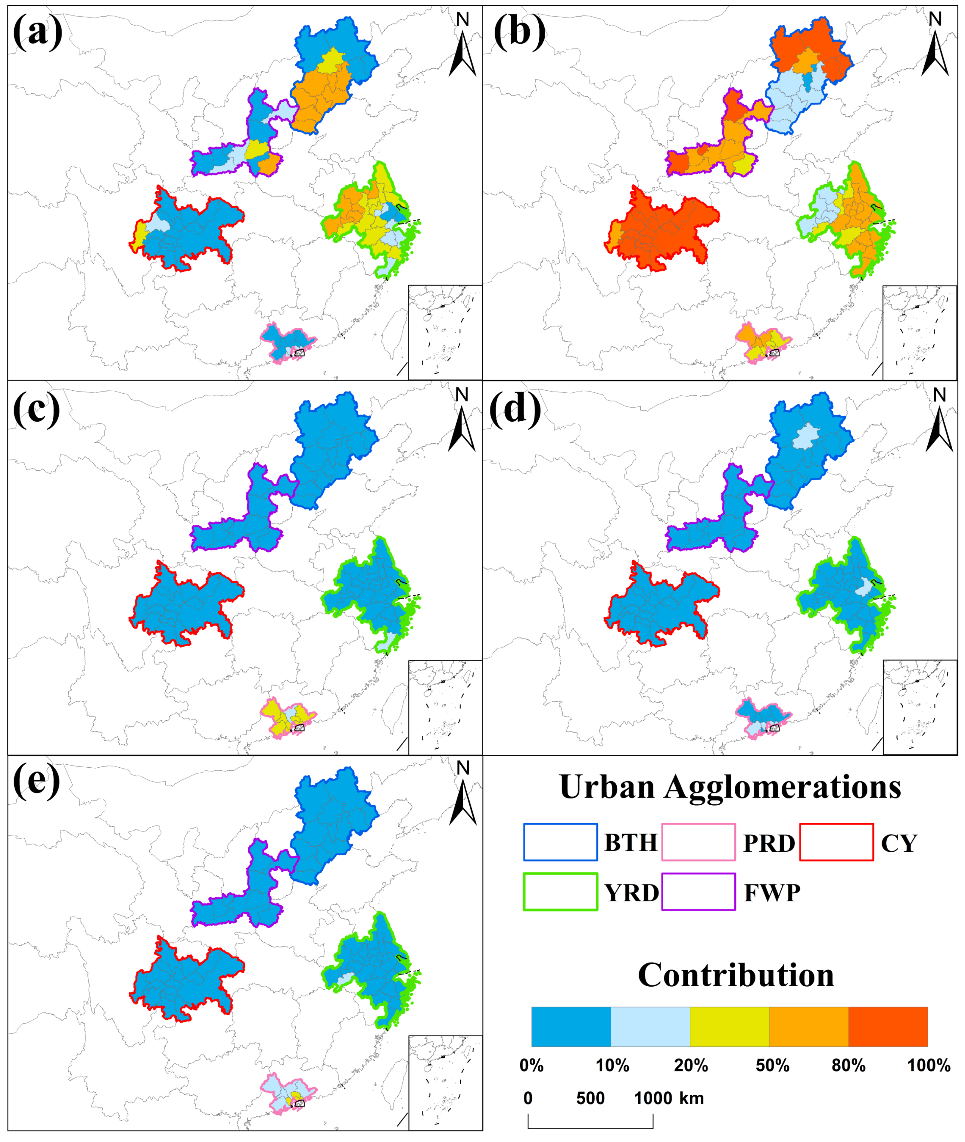
4.3. Emission Source Apportionment and Control Strategy Implications

The RF model’s high performance (R² = 0.962–0.987) validates the systematic influence of meteorological and emission factors on long-term O₃-8h trends. The wide meteorological contribution range in the YRD (10–40%) reflects its location in the East Asian monsoon transition zone, where synoptic weather variability drives photochemical conditions [54]. In contrast, the concentrated emission contributions in the FWP and CY (2–4%) indicate pollution regimes driven by rapid industrial growth (+12–18% annually since 2015), resembling earlier eastern industrialization phases.

Local emissions dominate in the YRD and FWP (53% each), suggesting that municipal-level controls on industrial, vehicular, and residential sources can yield immediate reductions [29]. Conversely, transport emissions dominate in the PRD (59%) and CY (55%), where local reductions are offset by 15–22% through regional inflow, necessitating coordinated airshed management [56]. These emission patterns interact with meteorological sensitivities, with BTH and YRD requiring seasonally adaptive controls to address temperature and radiation cycles, while FWP and CY need consistent year-round source reductions.

These findings underscore the need for differentiated control strategies: local source controls for the YRD and FWP, regional governance for the PRD and CY, and meteorologically adaptive measures for BTH. Future research should prioritize high-resolution emission inventories and integrated models to better capture regional pollution dynamics.

5. Conclusions

This study presents a comprehensive analysis of long-term O₃ pollution trends across 372 cities in China from 2013 to 2023, using a combination of KZ filtering and RF regression to quantify the relative impacts of meteorological conditions and emissions. The results reveal a clear east–west gradient in O₃-8h concentrations, with persistently high levels in eastern urban agglomerations, such as BTH, YRD, and PRD, primarily influenced by long-term emissions and meteorological factors. In contrast, inland regions, like FWP and CY, although exhibiting lower concentrations, have experienced a notable upward trend in recent years, driven by increased regional pollutant transport and sensitivity to short-term meteorological fluctuations.

T and UVB emerged as the dominant meteorological drivers in the northern and eastern regions, while the PRD region showed stronger influences from humidity and wind conditions. Emission contributions to O₃ trends were more prominent in the FWP and PRD, and further decomposition highlighted significant local emission impacts in BTH and YRD, alongside notable transport-related contributions in the PRD and CY.

These findings underscore the importance of region-specific O₃ mitigation strategies. In the eastern mega-city agglomerations (BTH, YRD), mitigation should concentrate on cutting VOC and NO_x emissions from petrochemical facilities and road traffic, with additional controls activated during heatwave periods when photochemical risk is highest. In the southwestern basins (CY, PRD), cross-provincial emission caps scaled to the transport share identified by the EOF analysis would balance local and regional responsibilities. For the FWP, a package of industrial restructuring—coal-to-gas substitution and kiln upgrades—combined with stagnation alert protocols is recommended to curb episodic ozone peaks. This study provides scientific evidence to support differentiated O₃ management strategies under complex atmospheric conditions in China.

References

1. Wang, Y.; Yang, Y.; Yuan, Q.; Li, T.; Zhou, Y.; Zong, L.; Wang, M.; Xie, Z.; Ho, H.C.; Gao, M.; et al. Substantially Underestimated Global Health Risks of Current Ozone Pollution. Nat. Commun. 2025, 16, 102. [Google Scholar] [CrossRef] [PubMed]
2. Akimoto, H. Global Air Quality and Pollution. Science 2003, 302, 1716–1719. [Google Scholar] [CrossRef] [PubMed]
3. Li, K.; Jacob, D.J.; Liao, H.; Zhu, J.; Shah, V.; Shen, L.; Bates, K.H.; Zhang, Q.; Zhai, S. A Two-Pollutant Strategy for Improving Ozone and Particulate Air Quality in China. Nat. Geosci. 2019, 12, 906–910. [Google Scholar] [CrossRef]
4. State Council. Air Pollution Prevention and Control Action Plan. 2013. Available online: http://www.gov.cn/zwgk/2013-09/12/content_2486773.htm (accessed on 28 February 2023).
5. Wang, Y.; Wild, O.; Chen, H.; Gao, M.; Wu, Q.; Qi, Y.; Chen, X.; Wang, Z. Acute and Chronic Health Impacts of PM2.5 in China and the Influence of Interannual Meteorological Variability. Atmos. Environ. 2020, 229, 117397. [Google Scholar] [CrossRef]
6. State Council. Three-Year Action Plan for Winning the Blue Sky Defense Battle. 2018. Available online: http://www.gov.cn/zhengce/content/2018-07/03/content_5303158.htm (accessed on 28 February 2023).
7. Li, G.; Bei, N.; Cao, J.; Wu, J.; Long, X.; Feng, T.; Dai, W.; Liu, S.; Zhang, Q.; Tie, X. Widespread and Persistent Ozone Pollution in Eastern China during the Non-Winter Season of 2015: Observations and Source Attributions. Atmos. Chem. Phys. 2017, 17, 2759–2774. [Google Scholar] [CrossRef]
8. Liu, Y.; Wang, T. Worsening Urban Ozone Pollution in China from 2013 to 2017–Part 2: The Effects of Emission Changes and Implications for Multi-Pollutant Control. Atmos. Chem. Phys. 2020, 20, 6323–6337. [Google Scholar] [CrossRef]
9. Mousavinezhad, S.; Choi, Y.; Pouyaei, A.; Ghahremanloo, M.; Nelson, D.L. A Comprehensive Investigation of Surface Ozone Pollution in China, 2015–2019: Separating the Contributions from Meteorology and Precursor Emissions. Atmos. Res. 2021, 257, 105599. [Google Scholar] [CrossRef]
10. Qu, Y.; Wang, T.; Cai, Y.; Wang, S.; Chen, P.; Li, S.; Li, M.; Yuan, C.; Wang, J.; Xu, S. Influence of Atmospheric Particulate Matter on Ozone in Nanjing, China: Observational Study and Mechanistic Analysis. Adv. Atmos. Sci. 2018, 35, 1381–1395. [Google Scholar] [CrossRef]
11. Wang, Y.; Gao, W.; Wang, S.; Song, T.; Gong, Z.; Ji, D.; Wang, L.; Liu, Z.; Tang, G.; Huo, Y.; et al. Contrasting Trends of PM2.5 and Surface-Ozone Concentrations in China from 2013 to 2017. Natl. Sci. Rev. 2020, 7, 1331–1339. [Google Scholar] [CrossRef]
12. Guha, S.; Zhang, T.; Kinney, P.L.; Henneman, L.R.F. Fine Particulate Matter and Ozone Variability with Regional and Local Meteorology in Beijing, China. Atmos. Environ. 2024, 338, 120793. [Google Scholar] [CrossRef]
13. Tao, J.; Zhang, L.; Cao, J.; Zhang, R. A Review of Current Knowledge Concerning PM2. 5 Chemical Composition, Aerosol Optical Properties and Their Relationships across China. Atmos. Chem. Phys. 2017, 17, 9485–9518. [Google Scholar] [CrossRef]
14. Li, K.; Jacob, D.J.; Liao, H.; Shen, L.; Zhang, Q.; Bates, K.H. Anthropogenic drivers of 2013–2017 trends in summer surface ozone in China. Proc. Natl. Acad. Sci. USA 2019, 116, 422–427. [Google Scholar] [CrossRef] [PubMed]
15. Lu, X.; Hong, J.; Zhang, L.; Cooper, O.R.; Schultz, M.G.; Xu, X.; Wang, T.; Gao, M.; Zhao, Y.; Zhang, Y. Severe Surface Ozone Pollution in China: A Global Perspective. Environ. Sci. Technol. Lett. 2018, 5, 487–494. [Google Scholar] [CrossRef]
16. Seinfeld, J.H.; Pandis, S.N.; Noone, K. Atmospheric Chemistry and Physics: From Air Pollution to Climate Change. Phys. Today 1998, 51, 88–90. [Google Scholar] [CrossRef]
17. Wang, Z.; Tan, Y.; Guo, M.; Cheng, M.; Gu, Y.; Chen, S.; Wu, X.; Chai, F. Prospect of China’s Ambient Air Quality Standards. J. Environ. Sci. 2023, 123, 255–269. [Google Scholar] [CrossRef]
18. Li, K.; Jacob, D.J.; Shen, L.; Lu, X.; De Smedt, I.; Liao, H. Increases in Surface Ozone Pollution in China from 2013 to 2019: Anthropogenic and Meteorological Influences. Atmos. Chem. Phys. 2020, 20, 11423–11433. [Google Scholar] [CrossRef]
19. Lelieveld, J.; Crutzen, P.J. Influences of Cloud Photochemical Processes on Tropospheric Ozone. Nature 1990, 343, 227–233. [Google Scholar] [CrossRef]
20. Dang, R.; Liao, H.; Fu, Y. Quantifying the Anthropogenic and Meteorological Influences on Summertime Surface Ozone in China over 2012–2017. Sci. Total Environ. 2021, 754, 142394. [Google Scholar] [CrossRef]
21. Wang, P.; Chen, K.; Zhu, S.; Wang, P.; Zhang, H. Severe Air Pollution Events Not Avoided by Reduced Anthropogenic Activities during COVID-19 Outbreak. Resour. Conserv. Recycl. 2020, 158, 104814. [Google Scholar] [CrossRef]
22. Ge, B.; Wang, Z.; Lin, W.; Xu, X.; Li, J.; Ji, D.; Ma, Z. Air Pollution over the North China Plain and Its Implication of Regional Transport: A New Sight from the Observed Evidences. Environ. Pollut. 2018, 234, 29–38. [Google Scholar] [CrossRef]
23. Li, M.; Geng, C.; Li, L.; Zheng, Z.; Xu, B.; Yang, W.; Wang, X. Meteorological Impacts on Surface Ozone: A Case Study Based on Kolmogorov–Zurbenko Filtering and Multiple Linear Regression. Front. Environ. Sci. 2023, 10, 1081453. [Google Scholar] [CrossRef]
24. Pearce, J.L.; Beringer, J.; Nicholls, N.; Hyndman, R.J.; Tapper, N.J. Quantifying the Influence of Local Meteorology on Air Quality Using Generalized Additive Models. Atmos. Environ. 2011, 45, 1328–1336. [Google Scholar] [CrossRef]
25. Wu, Y.; Liu, R.; Li, Y.; Dong, J.; Huang, Z.; Zheng, J.; Liu, S.C. Contributions of Meteorology and Anthropogenic Emissions to the Trends in Winter PM2.5 in Eastern China 2013–2018. Atmos. Chem. Phys. 2022, 22, 11945–11955. [Google Scholar] [CrossRef]
26. Xiao, Q.; Zheng, Y.; Geng, G.; Chen, C.; Huang, X.; Che, H.; Zhang, X.; He, K.; Zhang, Q. Separating emission and meteorological contributions to long-term PM₂.₅ trends over eastern China during 2000–2018. Atmos. Chem. Phys. 2021, 21, 9475–9496. [Google Scholar] [CrossRef]
27. Liu, X.; Niu, J.; Wang, Z.; Pan, X.; Su, F.; Yao, D.; Zhu, M.; Yan, J.; Yan, J.; Yao, G. A Comprehensive Investigation of PM2.5 in the Huaihe River Basin, China: Separating the Contributions from Meteorology and Emission Reductions. Atmos. Pollut. Res. 2023, 14, 101647. [Google Scholar] [CrossRef]
28. Niu, J.; Li, H.; Liu, X.; Lin, H.; Zhou, P.; Zhu, X. Driving Force of Meteorology and Emissions on PM2.5 Concentration in Major Urban Agglomerations in China. Atmosphere 2024, 15, 1499. [Google Scholar] [CrossRef]
29. Wu, L.; An, J. Quantitative Impacts of Meteorology and Emissions on the Long-Term Trend of O3 in the Yangtze River Delta (YRD), China from 2015 to 2022. J. Environ. Sci. 2025, 149, 314–329. [Google Scholar] [CrossRef]
30. Ding, J.; Dai, Q.; Fan, W.; Lu, M.; Zhang, Y.; Han, S.; Feng, Y. Impacts of Meteorology and Precursor Emission Change on O3 Variation in Tianjin, China from 2015 to 2021. J. Environ. Sci. 2023, 126, 506–516. [Google Scholar] [CrossRef]
31. Xiao, Q.; Geng, G.; Xue, T.; Liu, S.; Cai, C.; He, K.; Zhang, Q. Tracking PM2.5 and O3 Pollution and the Related Health Burden in China 2013–2020. Environ. Sci. Technol. 2022, 56, 6922–6932. [Google Scholar] [CrossRef]
32. Xue, T.; Zheng, Y.; Geng, G.; Xiao, Q.; Meng, X.; Wang, M.; Li, X.; Wu, N.; Zhang, Q.; Zhu, T. Estimating Spatiotemporal Variation in Ambient Ozone Exposure during 2013–2017 Using a Data-Fusion Model. Environ. Sci. Technol. 2020, 54, 14877–14888. [Google Scholar] [CrossRef]
33. Eskridge, R.E.; Ku, J.Y.; Rao, S.T.; Porter, P.S.; Zurbenko, I.G. Separating Different Scales of Motion in Time Series of Meteorological Variables. Bull. Amer. Meteor. Soc. 1997, 78, 1473–1483. [Google Scholar] [CrossRef]
34. Rao, S.T.; Zurbenko, I.G. Detecting and Tracking Changes in Ozone Air Quality. Air Waste 1994, 44, 1089–1092. [Google Scholar] [CrossRef]
35. Seo, J.; Park, D.-S.R.; Kim, J.Y.; Youn, D.; Lim, Y.B.; Kim, Y. Effects of Meteorology and Emissions on Urban Air Quality: A Quantitative Statistical Approach to Long-Term Records (1999–2016) in Seoul, South Korea. Atmos. Chem. Phys. 2018, 18, 16121–16137. [Google Scholar] [CrossRef]
36. Agudelo–Castaneda, D.M.; Calesso Teixeira, E.; Norte Pereira, F. Time–Series Analysis of Surface Ozone and Nitrogen Oxides Concentrations in an Urban Area at Brazil. Atmos. Pollut. Res. 2014, 5, 411–420. [Google Scholar] [CrossRef]
37. Gao, S.; Cheng, X.; Yu, J.; Chen, L.; Sun, Y.; Bai, Z.; Xu, H.; Azzi, M.; Zhao, H. Meteorological Influences on PM2.5 Variation in China Using a Hybrid Model of Machine Learning and the Kolmogorov-Zurbenko Filter. Atmos. Pollut. Res. 2023, 14, 101905. [Google Scholar] [CrossRef]
38. Sadeghi, B.; Ghahremanloo, M.; Mousavinezhad, S.; Lops, Y.; Pouyaei, A.; Choi, Y. Contributions of Meteorology to Ozone Variations: Application of Deep Learning and the Kolmogorov-Zurbenko Filter. Environ. Pollut. 2022, 310, 119863. [Google Scholar] [CrossRef]
39. Sun, X.; Zhao, T.; Bai, Y.; Kong, S.; Zheng, H.; Hu, W.; Ma, X.; Xiong, J. Meteorology Impact on PM2.5 Change over a Receptor Region in the Regional Transport of Air Pollutants: Observational Study of Recent Emission Reductions in Central China. Atmos. Chem. Phys. 2022, 22, 3579–3593. [Google Scholar] [CrossRef]
40. Zheng, H.; Kong, S.; Seo, J.; Yan, Y.; Cheng, Y.; Yao, L.; Wang, Y.; Zhao, T.; Harrison, R.M. Achievements and Challenges in Improving Air Quality in China: Analysis of the Long-Term Trends from 2014 to 2022. Environ. Int. 2024, 183, 108361. [Google Scholar] [CrossRef]
41. Breiman, L. Random forests. Mach. Learn. 2001, 45, 5–32. [Google Scholar] [CrossRef]
42. Yang, L.; Luo, H.; Yuan, Z.; Zheng, J.; Huang, Z.; Li, C.; Lin, X.; Louie, P.K.K.; Chen, D.; Bian, Y. Quantitative Impacts of Meteorology and Precursor Emission Changes on the Long-Term Trend of Ambient Ozone over the Pearl River Delta, China, and Implications for Ozone Control Strategy. Atmos. Chem. Phys. 2019, 19, 12901–12916. [Google Scholar] [CrossRef]
43. Zhou, L.; Zhang, J.; Lu, T.; Bao, M.; Deng, X.; Hu, X. Pollution Patterns and Their Meteorological Analysis All over China. Atmos. Environ. 2021, 246, 118108. [Google Scholar] [CrossRef]
44. Zhan, C.; Xie, M.; Liu, J.; Wang, T.; Xu, M.; Chen, B.; Li, S.; Zhuang, B.; Li, M. Surface Ozone in the Yangtze River Delta, China: A Synthesis of Basic Features, Meteorological Driving Factors, and Health Impacts. J. Geophys. Res. Atmos. 2021, 126, e2020JD033600. [Google Scholar] [CrossRef]
45. Xu, J.; Zhang, Z.; Zhao, X.; Zhang, J. Synthetically Impacts of the Topography and Typhoon Periphery on the Atmospheric Boundary Layer Structure and Special Regional Pollution Pattern of O3 in North China Plain. Atmos. Environ. 2024, 330, 120566. [Google Scholar] [CrossRef]
46. Li, Y.; Wang, T.; Wang, Q.; Li, M.; Qu, Y.; Wu, H.; Fan, J.; Shao, M.; Xie, M. Deciphering the Seasonal Dynamics of Multifaceted Aerosol-Ozone Interplay: Implications for Air Quality Management in Eastern China. Sci. Total Environ. 2024, 946, 174327. [Google Scholar] [CrossRef]
47. Alduwais, A.K.; Dasari, H.P.; Karumuri, R.K.; Gandham, H.; Koteswararao, V.; Saharwardi, M.S.; Ashok, K.; Hoteit, I. Spatiotemporal Variability of Surface Ozone and Associated Meteorological Conditions over the Arabian Peninsula. Atmos. Pollut. Res. 2024, 15, 102210. [Google Scholar] [CrossRef]
48. Lu, X.; Zhang, L.; Chen, Y.; Zhou, M.; Zheng, B.; Li, K.; Liu, Y.; Lin, J.; Fu, T.-M.; Zhang, Q. Interannual and decadal changes in tropospheric ozone in China and the associated chemistry-climate interactions: A review. Advances in Atmospheric Sciences 2019, 36, 1087–1106. [Google Scholar] [CrossRef]
49. Tabunshchik, V.; Nikiforova, A.; Lineva, N.; Drygval, P.; Gorbunov, R.; Gorbunova, T.; Kerimov, I.; Pham, C.N.; Bratanov, N.; Kiseleva, M. The Dynamics of Air Pollution in the Southwestern Part of the Caspian Sea Basin (Based on the Analysis of Sentinel-5 Satellite Data Utilizing the Google Earth Engine Cloud-Computing Platform). Atmosphere 2024, 15, 1371. [Google Scholar] [CrossRef]
50. Xu, J.; Zhao, Z.; Wu, Y.; Zhang, Y.; Wang, Y.; Su, B.; Liang, Y.; Hu, T.; Liu, R. Impacts of Meteorological Conditions on Autumn Surface Ozone During 2014–2020 in the Pearl River Delta, China. Earth Space Sci. 2023, 10, e2022EA002742. [Google Scholar] [CrossRef]
51. Li, H.; Yang, Y.; Su, H.; Wang, H.; Wang, P.; Liao, H. Ozone Pollution in China Affected by Climate Change in a Carbon Neutral Future as Predicted by a Process-Based Interpretable Machine Learning Method. Geophys. Res. Lett. 2024, 51, e2024GL109520. [Google Scholar] [CrossRef]
52. Xu, J.; Huang, X.; Wang, N.; Li, Y.; Ding, A. Understanding Ozone Pollution in the Yangtze River Delta of Eastern China from the Perspective of Diurnal Cycles. Sci. Total Environ. 2021, 752, 141928. [Google Scholar] [CrossRef]
53. Zhang, X.; Xu, W.; Zhang, G.; Lin, W.; Zhao, H.; Ren, S.; Zhou, G.; Chen, J.; Xu, X. First Long-Term Surface Ozone Variations at an Agricultural Site in the North China Plain: Evolution under Changing Meteorology and Emissions. Sci. Total Environ. 2023, 860, 160520. [Google Scholar] [CrossRef]
54. Zhao, Z.; Wang, Y. Influence of the West Pacific Subtropical High on Surface Ozone Daily Variability in Summertime over Eastern China. Atmos. Environ. 2017, 170, 197–204. [Google Scholar] [CrossRef]
55. Shao, T.; Wang, P.; Yu, W.; Gao, Y.; Zhu, S.; Zhang, Y.; Hu, D.; Zhang, B.; Zhang, H. Drivers of Alleviated PM2.5 and O3 Concentrations in China from 2013 to 2020. Resour. Conserv. Recycl. 2023, 197, 107110. [Google Scholar] [CrossRef]
56. Liu, M.; Ma, M.; Liu, M.; Meng, F.; Fu, P.; Xing, H.; Bi, J.; Zheng, Z.; Lv, Y. Quantitative Estimation of the Impacts of Precursor Emissions on Surface O3 and PM2.5 Collaborative Pollution in Three Typical Regions of China via Multi-Task Learning. Sustainability 2024, 16, 2475. [Google Scholar] [CrossRef]
Figure 1. Distribution of the five urban agglomerations. Agglomeration outlines: BTH = Beijing–Tianjin–Hebei (blue), YRD = Yangtze River Delta (green), PRD = Pearl River Delta (pink), FWP = Fenwei Plain (purple), CY = Chengdu–Chongqing (red). The data on terrain elevation are available at https://www.earthdata.nasa.gov/about/competitive-programs/measures/new-nasa-digital-elevation-model, accessed on 30 October 2024.
Atmosphere 16 00768 g001
Figure 2. Spatial distribution of O3-8h in China: (a) 2013–2017, (b) 2018–2020, (c) 2021–2023.
Atmosphere 16 00768 g002
Figure 3. Spatial distribution of O3-8h in China (2013–2023): (a) spring (March–May), (b) summer (June–August), (c) autumn (September–November), and (d) winter (December–February).
Atmosphere 16 00768 g003
Figure 4. Percentage contributions from KZ filter decomposition: (a) XST, (b) XSN, and (c) XLT components.
Atmosphere 16 00768 g004
Figure 5. (a) The 2013–2023 nationwide average O3-8h KZ filter results and the (b) BTH, (c) YRD, (d) PRD, (e) FWP, (f) and CY KZ filter results.
Atmosphere 16 00768 g005
Figure 6. Spatial distribution of normalized percentage contributions of key meteorological factors to long-term O3-8h concentrations estimated using the random forest model: (a) T, (b) UVB, (c) RH, (d) PS, and (e) WS.
Atmosphere 16 00768 g006
Figure 7. Relationship between meteorological and emission contributions to long-term O3-8h trends in five urban agglomerations.
Atmosphere 16 00768 g007
Figure 8. Spatial distribution of relative contributions to long-term O3-8h concentration trends. (a) Contribution of meteorological factors (MET); (b) contribution of overall emission factors (EMIS); (c) relative contribution of local emissions (EMIS(L)) to O3-8h; (d) relative contribution of transport-related emissions (EMIS(T)) to O3-8h.
Atmosphere 16 00768 g008
Figure 9. Relative contributions of local (EMIS(L)) and transport-related (EMIS(T)) emissions to long-term O3-8h trends in five urban agglomerations.
Atmosphere 16 00768 g009