Assessment of CH₄ and CO₂ Emissions from a Municipal Waste Landfill: Trends, Dispersion, and Environmental Implications

Abstract

The European Union views biogas production from landfills as a crucial element in achieving decarbonization goals by 2050. Biogas is primarily composed of methane (CH₄) and carbon dioxide (CO₂), produced through the anaerobic digestion of various residual materials. This study aimed to investigate CH₄ and CO₂ concentrations from municipal solid waste in biogas capture wells in a landfill in Romania between 2023 and 2024. A peak in CH₄ concentrations occurred in the fall of 2024 (P4 well), while the highest CO₂ content was recorded in the summer of 2023 (P3 well). The Aermod View software platform (version 11.2.0) was employed to model the dispersion of pollutants in the surrounding air. A worst-case scenario was applied to estimate the highest ground-level pollutant concentrations. The highest recorded CH₄ concentration was 90.1 mg/m³, while CO₂ reached 249 mg/m³ within the landfill. The highest CH₄ concentrations were found in the southern part of the site, less than 1 km from the landfill, while CO₂ was highest in the northern area. In conclusion, municipal solid waste landfills behave like unpredictable bioreactors, and without proper management and oversight, they can pose significant risks. An integrated system that combines prevention, reuse, and correct disposal is critical to minimizing these negative effects.

1. Introduction

1.1. Research Background

Waste disposal sites are a major source of anthropogenic greenhouse gases (GHGs), the most prevalent being methane (CH₄) and carbon dioxide (CO₂). CH₄ is a GHG with a global warming potential 28 times higher than that of CO₂ [1]. Methane contributes to global warming and is the second most potent GHG produced by human activities, following CO₂ [2]. Over the last century, the global warming potential of methane has become approximately 30 times greater than that of CO₂ [1].

Landfills constitute the third largest human-made source of CH₄ emissions to the atmosphere worldwide [3,4,5,6]. Globally, landfills contribute significantly to CH₄ emissions, representing up to 40% of the total estimated CH₄ emissions in specific environments [7].

In Europe, more than 1 billion tons of waste are produced annually, with the largest share coming from construction and municipal waste management [8].

GHG emissions due to the incorrect handling of municipal solid waste (MSW) represent one of the major concerns for both growing and developed countries [8].

The generation and management of municipal waste represent an increasingly pressing issue with major ecological, economic, and social implications. The global average waste generation is about 0.74 kg per capita per day, with variations between 0.11 and 4.54 kg per capita per day, depending on the country [9]. By 2025, the volume of MSW is estimated to reach 2.2 billion tons, with over one-third remaining uncollected [9]. By 2050, global municipal solid waste (MSW) generation is projected to reach 3.4 billion metric tons per year, representing a 70% increase from 2016 levels [9]. High-income countries contribute an increase of ~19% (driven by high per capita waste generation), and low- and middle-income countries contribute ~40% or more (due to urbanization, population growth, and increased consumption). Most MSW originates from everyday activities, primarily generated by residential, commercial, and institutional sources [10,11].

Scientific research has demonstrated that the volume of waste produced grows proportionally with economic development, a phenomenon particularly observed in developing countries [9,12].

Kaza et al. indicate that landfilling is the most economically, technically, and socially feasible method of solid waste management in developing countries [9], even if is considered the most harmful method and ranks on the end in the waste management hierarchy, increasing environmental impact [13]. Additionally, inefficient landfill management creates major issues, such as gas emissions and the generation of large quantities of leachate [6].

Biogas generation in MSW landfills involves a biologically mediated process in which microorganisms break down organic materials in waste in the presence of an electron acceptor (oxygen, nitrates, etc.), producing new biomass, heat, and biogas (CH₄ and CO₂). Depending on the availability of oxygen, decomposition can be aerobic or anaerobic [14,15]. The process of disposing of municipal solid waste in landfills generates three primary by-products: gas, leachate, and heat. Depending on the availability of oxygen, decomposition can be aerobic or anaerobic [14,15].

The gas produced through anaerobic digestion, known as biogas, consists of two main components: CH₄ (45–60%) and CO₂ (40–60%), Additionally, there are minor components (0.1–5%) such as oxygen, hydrogen, nitrogen, carbon monoxide, sulfides, and ammonia, along with various trace components (0.01–0.6%) [4,8,14,16,17,18,19,20]. The GHG content depends on the quantity of stored waste, its chemical composition, and the landfill’s humidity. CH₄ concentration is approximately 1.25 times that of CO₂, a ratio that differs from the composition of biogas generated in wastewater treatment plants [8,13].

The factors influencing the transport processes of biogas, which lead to the migration and emission of CH₄, can be grouped into three categories: meteorological conditions such as barometric pressure, precipitation, temperature, and wind; soil and cover conditions including cracks, fissures, permeability, diffusivity, porosity, moisture content, organic matter, and CH₄ oxidation capacity; and waste composition and landfill conditions such as age, gas production rate, internal barriers, and lateral migration zones [18]. The process is affected by factors such as the quantity, composition, and age of the waste, pH, humidity, waste mass temperature, and oxygen penetration, along with landfill design and operations. Biogas generation varies spatially, leading to different pressures within the waste mass [14].

Barometric pressure is one of the most extensively examined meteorological variables. Prior studies identified it as the primary factor influencing CH₄ emission rates at the decommissioned Park Road Landfill in Grimsby, Ontario, Canada [21]. Studies indicate that precipitation reduces biogas flux in the short term, as water fills soil pores; however, methane emissions tend to increase later as the pores drain and gas diffusion resumes [22]. Spatial and temporal variations in the physical and chemical properties of the soil, which influence biogas transport in the soil and microbial activity (composition, depth, moisture, temperature, aeration status), are particularly important [18,19].

Landfills continuously receive waste over many years. Once municipal solid waste is deposited in such a facility, it undergoes a series of biological, chemical, and physical transformations [23,24]. Anaerobic decomposition depends on the symbiotic interaction of three main types of bacteria, hydrolytic/fermentative, acetogenic, and methanogenic, each with a specific role [25]. The decomposition of waste is characterized by five distinct phases, initial adjustment, transition, acid generation, methanogenesis, and final maturation, as illustrated in Figure 1 [10].

The initial adjustment or aerobic decomposition stage (I) begins with waste deposition and moisture accumulation, when oxygen trapped in the voids between wastes supports microbial activity, generating CO₂ and water until the oxygen is depleted [10,26].

The transition or acidogenic stage (II) marks the shift to an anaerobic environment, where oxygen is replaced by nitrates and sulfates, and CO₂ becomes dominant, establishing reductive conditions and leading to the accumulation of organic compounds in the leachate [10,26].

In the acid generation stage (III), fermentation and hydrolysis intensify microbial activity, leading to the production of volatile organic acids (VOAs), CO₂, and H₂, a rise in Chemical Oxygen Demand (COD) and Biological Oxygen Demand (BOD), and the mobilization of heavy metals due to the decrease in pH [10,26].

The biodegradation of organic matter, which involves the action of methanogenic bacteria, converts organic acids and intermediates generated in the previous stages into CH₄ and CO₂ (stage IV) [10,26]. Methane gas production increases as the pH becomes nearly neutral (6.8–8.0), and the leachate’s pollutant concentration decreases [10,26].

The maturation stage (V) represents the final stabilization stage, during which the remaining degradable materials decompose slowly, generating only small amounts of gas. The substrates become dominated by humic and fulvic acids, and microbial activity slows significantly [10,26].

1.2. Literature Review

Methane from landfills has a greenhouse effect approximately 28 times greater per kilogram of emissions than carbon dioxide over a 100-year period [27]. The United Nations Environment Programme (UNEP) in 2023 established the need to reduce anthropogenic methane emissions by 45% in the near future. This reduction would prevent global warming by nearly 0.3 °C by 2045 and align with the Paris Climate Agreement’s goal of limiting the global temperature increase to 1.5 °C [2]. However, by 2050, greenhouse gas emissions from landfills are projected to increase by approximately 1.5 times their current levels, reaching around 2400 MtCO₂e [17].

Analyzing epidemiological studies, there is evidence that continuous inhalation of CH₄ and CO₂ can cause nausea, vomiting, headaches, loss of coordination, and increased blood pressure. At very high levels of exposure, methane can lead to comas and death by asphyxiation [28]. In addition, CH₄ is known to be extremely flammable and capable of causing explosions when its concentration in air reaches between 5% and 15% [28].

In the United States (US), landfills accounted for 17% of methane emissions in 2022, with the majority of these emissions coming from MSW landfills [29]. The U.S. Environmental Protection Agency (EPA) has identified reducing methane emissions from MSW landfills as an important priority for regulatory enforcement during the 2024–2027 period [30]. A US EPA report attributes 58% of methane emissions from MSW landfills to food waste [31]. As waste is deposited, it decomposes and produces CH₄. Although daily cover is applied to control odor and pests, it does not address gas capture. In cases where the waste is older than five years, gas collection systems may not be active. Additionally, gas wells may be turned off when new waste is added on top of older layers, or their efficiency may be reduced to avoid introducing excess oxygen into the waste mass, which leads to CH₄ leaks into the atmosphere [31].

In Thailand, with a tropical equatorial climate, 78% of solid waste disposal sites are open dumps. Emissions are significantly higher during the rainy season, with the greatest difference observed in controlled landfills [32].

In Florida, model adjustments to direct flow measurements indicate potential values of methane generation between 56 m³ CH₄/Mg MSW and 77 m³ CH₄/Mg MSW, while degradation constants range from 0.04 to 0.13 per year [33].

In the United Kingdom, the landfill tax—introduced as part of efforts to meet waste reduction targets under the EU Landfill Directive—has progressively increased from GBP 7 per tons in 1996 to GBP 82.60 per tons by 2015, rendering landfilling a less economically viable option. Consequently, the proportion of MSW landfilled declined from 70% in 2004 to 34% in 2013. Despite this reduction, the UK still lags behind other EU countries such as Germany and the Netherlands, where less than 2% of MSW is landfilled. The share of waste incinerated with energy recovery also remains comparatively low in the UK (21%) relative to Germany and the Netherlands, which incinerate approximately 35% and 49% of MSW, respectively [34].

1.3. Research Innovation

The environmental performance of MSW management systems has been extensively evaluated through life cycle assessment (LCA) methodologies. The goal of the bioeconomy is to integrate biomass and organic waste into key production sectors such as agriculture, forestry, and fishing, while efficiently utilizing raw materials in order to reuse/recycle/reduce/recover [35]. The 4Rs of sustainable waste management are fundamental principles designed to minimize environmental impact and promote resource efficiency.

To reduce emissions from landfills, it is necessary to upgrade landfill operations and implement efficient systems for the collection and utilization of biogas. Producing biogas from waste is a well-established and effective method for energy utilization and reducing greenhouse gas emissions [10,17,18].

Biogas production increases with the amount of biodegradable organic materials, particularly food and green waste, which favor anaerobic decomposition. The main components include sugars, starches, cellulose, and hemicellulose, while the most resistant are proteins, nucleic acids, lipids, and lignocellulose [14].

A landfill can produce emissions of approximately 15–25 L/kg of biogas per year during its operational lifespan [36]. This biogas can be utilized as fuel for energy production, and the collected biogas can be provided to suitable nearby industries for direct use in sectors such as internal combustion engines and gas turbines, microturbines, steam boilers, and other facilities [37].

To reduce leachate production and protect groundwater resources, modern municipal solid waste (MSW) landfills are equipped with composite covers, including compacted clay, a flexible membrane liner, a drainage layer, and soil for vegetation support. These covers are impermeable to gases and include gas collection systems and atmospheric ventilation [11].

Microbial oxidation of CH₄ in the landfill cover layers can significantly reduce methane emissions, and the efficiency of this process depends on factors such as soil moisture, temperature, and ammonium nitrogen content. Studies have shown that soil biofilters can be effective in oxidizing CH₄, provided the environment supports the development of methanotrophs [38].

Many studies around the world have proposed solutions in order to manage municipal waste landfills, with focus on biogas capture and leachate treatment. Figure 2 illustrates the technological process applied for waste management according to the literature data [39,40,41].

Romania faces huge problems related to municipal landfills. The most widely used method of waste disposal is landfills; thus, it is essential to assess the extent to which the gases produced in these landfills can disperse into the surrounding areas. More than 75% of the municipal wastes produced in Romania, according to statistics from 2016 to 2020, are landfilled [42]. Smaller percentages are incinerated, recycled, or composted and digested [42]. Data from 2020 indicated more than 4 million tons of municipal wastes were collected and stored in the landfills, representing around 79% from the total municipal wastes produced. The rest of the quantity up to 5.5 million tons was incinerated (4.6%), recycled (9.1%), and composted (7.3%) [42].

The most common method of waste disposal is in landfills, which is why it is crucial to evaluate how far the gases generated in these landfills can spread into the surrounding areas. In this context, monitoring air quality around such municipal waste landfills is necessary in order to prevent contamination of the soil and groundwater, as well as to ensure high air quality for residential areas in the area of influence.

This article addresses several important gaps in the existing literature, particularly regarding the modeling of GHG (CH₄ and CO₂) dispersion from waste landfill sites under specific local conditions in Romania. While many international studies focus on heavily industrialized regions or different pollutants, this study contributes valuable data and modeling insights from an under-represented Eastern European context.

In this context, the purpose of the study was to examine the impact of a selected municipal landfill located in Romania. To assess the impact, variations of CH₄ and CO₂ gases were investigated for the period 2023–2024.

2. Materials and Methods

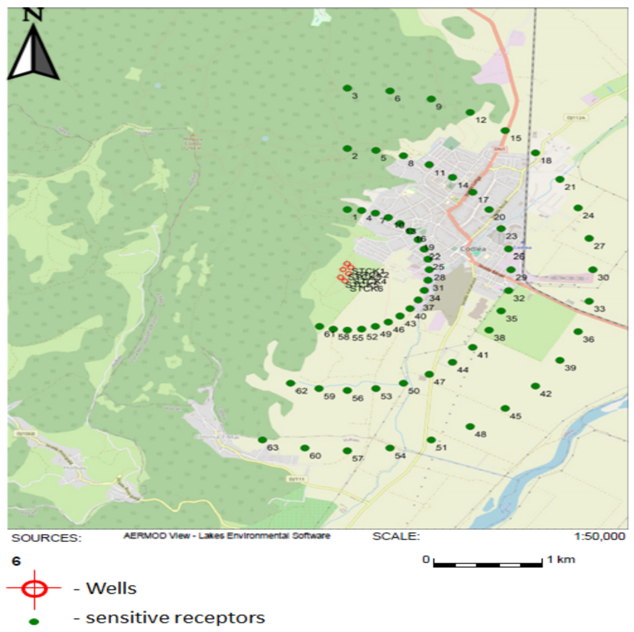
2.1. Description of the Landfill Location and the Main Sampling Points

The selected solid waste landfill is located in Romania, in a region characterized by a temperate oceanic climate and a temperate continental climate, which is generally more humid and colder, situated at approximatively 0.6 km from the closest sensitive receptors, at the border of the municipality.

The landfill was opened in 1979 and, being non-compliant, was closed in 2009. It occupies an area of 2.87 hectares, with a capacity of 200,000 cubic meters and a maximum height of approximately 18 m from its base. The types of waste deposited included household waste and construction debris.

The impermeabilization of the landfill was carried out as follows: over the leveled surface, a final closure system was installed, consisting of the following layers: a 15 cm vegetative layer, 85 cm of recultivation soil, permeable geotextile, a 30 cm rainwater drainage layer (gravel 16/31.5 mm), bentonite geocomposite (6000 g/m²), geotextile (400 mg/m²), and a 50 cm gas drainage layer (gravel 16/31.5 mm).

The gas extraction wells (six wells, P1–P6) are equipped with biofilters at the top, which reduce the environmental impact of biogas and eliminate the risk of explosion within the site. These wells are installed inside the landfill body, within the mass of waste that generates gas. The wells are symmetrically placed at a recommended distance of 50 m from each other. They are positioned as close as possible to protective and stability embankments within the landfill and to access roads. The distance from the wells to the outer edge of the landfill needs to be greater than 40 m, in order to include the edge of the landfill in the gas extraction zone.

The biogas collection wells consist of a vertical filter with a diameter greater than 80 cm, made of gravel or crushed stone (16–31.5 mm), into which a drainage pipe with an internal diameter of at least 200 mm is embedded. The walls of the filter pipes are perforated with round holes of 8–12 mm in diameter. The biogas wells are installed approximately 4 m above the base of the landfill, and the bottom of each well must be located at least 2–3 m above the leachate drainage layer.

These measures were implemented as environmental obligations imposed through the Environmental Impact Assessment (AIM), in accordance with in force legislation [43,44].

A total number of 63 points were placed around the landfill on three semicircles at a distance of 0.2 and 0.6 km from the landfill central point. Their spatial distribution is illustrated in Figure 3.

On the west and northwest of the municipal landfill site is located a rich forest that acts as a natural barrier to the pollutant dispersion (Figure 3).

Figure 4A presents images from the municipal solid waste storage station site, providing a visual overview of the landfill’s infrastructure and operations. Additionally, it highlights the measurement process for CH₄ and CO₂ concentrations from the biogas capture well (Figure 4B).

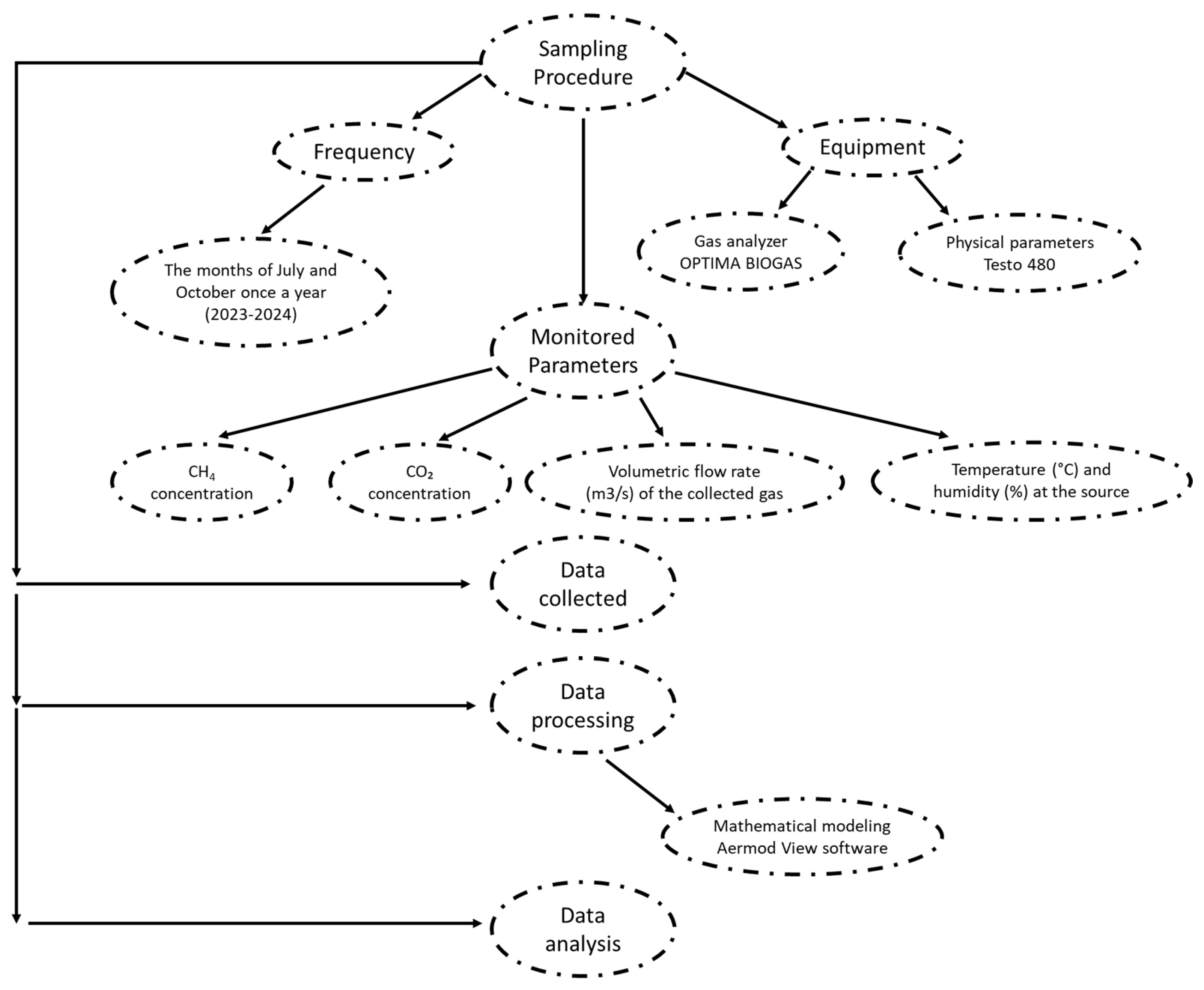
2.2. Methodology Applied

The study was conducted with the objective of assessing seasonal variation, comparing pollutant dispersion during summer and autumn for the years 2023 and 2024, specifically in July and October, once per year. The use of a worst-case scenario ensured that potential seasonal differences could be analyzed under the most conservative conditions, providing robust comparative insights even without percentile-based scenarios.

The AERMOD dispersion model was applied using a worst-case scenario, incorporating meteorological conditions and emission parameters expected to produce maximum ground-level concentrations of pollutants (CH₄ and CO₂). This conservative approach is consistent with the regulatory framework of the US EPA and the European Environment Agency (EEA) [45], and is commonly used to ensure a high level of precaution in environmental assessments.

At the beginning of the measurement campaign, a sampling plan was developed, which included the identification of emission sources, their positioning, and the measurement of their dimensions (diameter 0.86 m and height 1.65 m). The strategy for measuring pollutant concentrations and physical parameters was also established. During each measurement campaign, the concentrations of the two pollutants were measured simultaneously with the physical parameters of the emission sources (velocity, temperature, and humidity). The physical parameters (velocity, temperature, humidity) of the gaseous effluents from the emission sources were measured as hourly averages, based on 4 individual 15 min measurements taken at each emission source. The volumetric flow rate of each emission source was calculated using the average of the measured physical parameters. The collected data has been analyzed using mathematical modeling, interpretation of meteorological data, and dispersion simulations for CH₄ and CO₂. The results have been presented in semi-annual reports, with all data to be compared and evaluated at the end of the monitoring period.

Figure 5 presents the methodology applied for sampling, collection, and processing the data in order to estimate the emission of pollutants from the municipal waste landfill.

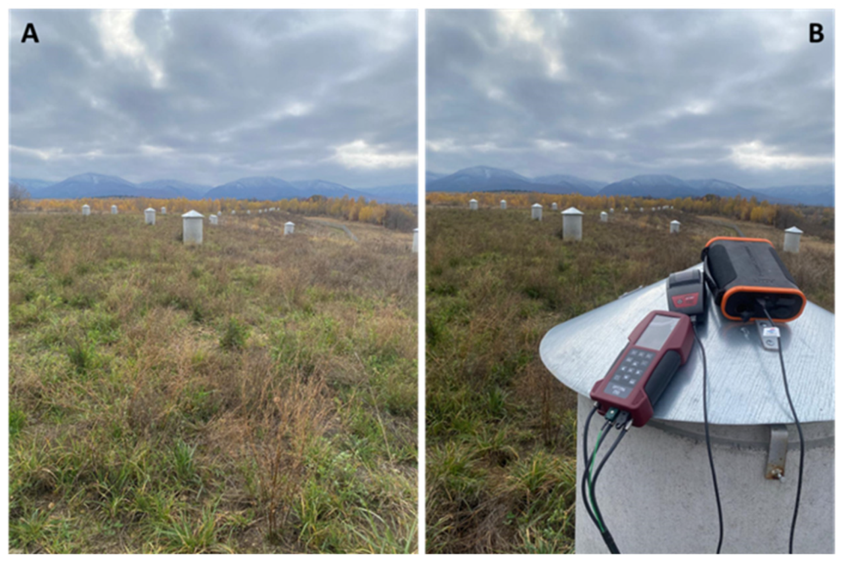
2.3. CH₄ and CO₂ Measurements

Gas monitoring was carried out using a biogas analyzer model OPTIMA BIOGAS (MRU GmbH, Neckarsulm-Obereisesheim, Germany), a multifunctional analyzer used for the simultaneous measurement of biogas composition and parameters related to emissions and combustion. The technical specifications of the biogas analyzer highlight its ability to accurately measure key gas components. Methane (CH₄) and carbon dioxide (CO₂) are measured using the NDIR (non-dispersive infrared) method, ensuring reliable and fast detection. The measuring range for both gases spans from 0 to 100%, with a high resolution of 0.01%, allowing for the detection of even minor changes in gas composition. The measurement accuracy is ±0.3%, providing a high level of confidence in the results, crucial for effective monitoring and optimization of biogas production processes.

The biogas analyzer has various applications in monitoring industrial and environmental processes. Among its key functionalities are the detection and measurement of oxygen (O₂), CH₄, CO₂, hydrogen sulfide (H₂S), and, optionally, biogas pressure. The device can also be used for advanced combustion process measurements in engines, analyzing parameters such as O₂, CO, NO, NO₂, and CO₂, including the calculation of NOx (NO + NO₂) concentrations expressed in mg/m³ and normalized to user-defined values [46].

2.4. Meteorological Data Used

Meteorological data used as input were provided by the Romanian National Meteorological Administration (RNMA) and consisted of validated meteorological records [47]. The meteorological station is located approximately 8 km from the municipal waste landfill. These data characterize six meteorological parameters (temperature, pressure, humidity, cloud cover, wind speed, and wind direction) and were provided as hourly averages, following the dispersion program’s requirements.

Meteorological data were statistically processed using AERMET View (version 11.2.0) to eliminate outlier values and generate the wind rose diagrams (Figure 6A,B), which depict the period’s wind direction distribution in a “blowing from” format.

The distribution of the wind speed frequency, data collected from RNMA, is presented in Figure 7A,B for both seasons.

2.5. Mathematical Modeling Description

The emission source parameters, meteorological data, and receptor characteristics were used as input data in the model to simulate the hourly average concentration distributions at ground level for CH₄ and CO₂ during the two seasons, summer and autumn (specifically the months of July and October).

The highest ground-level concentrations of CH₄ and CO₂ emissions from the landfill were estimated for gas emission simulations based on mathematical modeling.

The Aermod View software platform, version 11.2.0, was used to simulate the dispersion of pollutants in the air surrounding the landfill. AERMOD View uses the enhanced Gaussian dispersion model AERMOD, developed by the U.S. EPA and AMS, as its core mathematical model. It is a steady-state air dispersion model based on planetary boundary layer theory, accounting for various meteorological conditions, complex terrain, and building downwash effects (via the PRIME algorithm). It incorporates advanced parameters such as atmospheric stability, wind friction, and potential temperature. Data processing is handled through AERMET (meteorological data), AERMAP (terrain), providing detailed and accurate air pollutant dispersion estimates. AERMET and AERMAP are parts of the Aermod View software platform, version 11.2.0.

The model was applied to assess the spatial distribution of methane (CH₄) and carbon dioxide (CO₂) emissions. Interpolation was carried out automatically by the software over a defined computational grid, based on input parameters such as meteorological data, terrain characteristics, and emission source properties. The resulting concentration fields were visualized as isoconcentration contour maps, representing the estimated ground-level concentrations of CH₄ and CO₂ across the study area.

The dispersion modeling of pollutants was carried out using AERMOD View (version 11.2.0), with the following key settings and parameters:

• Terrain settings: A digital elevation model Stereographic coordinate system 1970 (SRTM 30) was used to account for topographic variations within the study area. These data were processed using the AERMAP preprocessor, which assigns elevation values and hill height scales to each receptor based on surrounding terrain features.
• Model parameters:

  ◦

  Source type: (e.g., point source, area source, or volume source depending on the emission characteristics);

  ◦

  Stack height (m);

  ◦

  Emission rate of CH₄ and CO₂ (g/s);

  ◦

  Meteorological parameters: wind speed at 10 m, wind direction, temperature, humidity, and wind frequency distribution;

  ◦

  Modeling domain: defined using a Cartesian receptor grid with appropriate resolution;

  ◦

  Receptor height: typically set at 1.5 m to represent average breathing height.

The maps presented in Section 3 were developed using the Stereo 70 (Stereographic 1970) coordinate system, based on a local Cartesian projection (

Table 1. Parameters of Stereo 70 coordinate system.

Feature	Stereo 70 (Meters)	DMS (Degrees, Minutes, Seconds)
Units	Meters (Cartesian)	Angular (degrees)
Best for	Mapping, cadastral, GIS	GPS display, global positioning
Distance and area	Easy to calculate	Requires conversion
Romanian compatibility	Official standard	Requires conversion
Software compatibility	Excellent (GIS, CAD)	Limited

). This system ensures high accuracy for national-scale mapping and is the official geodetic reference used in Romania for cadastral, topographic, and infrastructure-related applications.

For each type of simulation, dispersion maps were generated, and maximum concentrations of gaseous pollutants were obtained by applying Uniform Cartesian Grid receptors across the entire dispersion map area, with a total of 63 points introduced (Figure 3).

Aermod View uses an atmospheric dispersion model driven by turbulence structure of atmospheric layers and scaling concepts, including the handling of multiple point sources at ground level or at height. It can be applied to flat or complex terrain, in rural or urban settings, and includes algorithms for building-induced effects. The model employs Gaussian dispersion for stable atmospheric conditions and non-Gaussian models for unstable conditions. Dispersion simulation in complex terrain is performed using streamline separation procedures, allowing pollutants to move over or around landforms depending on the height of the pollutant plume and stability conditions.

The “Highest values” function was used, corresponding to the top 2% of values over one period (43.68 h). This situation represents the most unfavorable meteorological and emission conditions, presenting the highest estimated ground-level value as an hourly average under the worst-case emission and dispersion scenarios for an entire year.

The most unfavorable meteorological conditions are a stable atmosphere (classes E and F), low wind speeds, thermal inversions, and reduced turbulence. These conditions frequently occur at night and limit pollutant dispersion, promoting their accumulation near the source, especially in low-lying or enclosed terrain.

3. Results and Analysis

3.1. Physical Parameters from Emission Sources

Table 2. Physical parameters determined at the emission sources over the years 2023–2024.

Period	Sources	Volumetric Flow Rate, m3/s	Velocity, m/s	Temperature, °C	Humidity, %
Summer 2023	P1 Well	0.035	0.06024	18.1	81.2
	P2 Well	0.007	0.01205	19.4	82.5
	P3 Well	0.007	0.01205	84.6	20.7
	P4 Well	0.035	0.06024	-	-
	P5 Well	0.049	0.08434	-	-
	P6 Well	0.064	0.11015	-	-
Autumn 2023	P1 Well	0.007	0.01205	17.9	73.4
	P2 Well	0.007	0.01205	21.3	69.3
	P3 Well	0.007	0.01205	23.1	81.2
	P4 Well	0.007	0.01205	-	-
	P5 Well	0.007	0.01205	-	-
	P6 Well	0.007	0.01205	-	-
Summer 2024	P1 Well	0.007	0.01205	22.6	63.5
	P2 Well	0.007	0.01205	24.5	70.7
	P3 Well	0.007	0.01205	21.9	68.4
	P4 Well	0.007	0.01205	23.5	69.5
	P5 Well	0.007	0.01205	26.7	71.3
	P6 Well	0.007	0.01205	24.4	70.5
Autumn 2024	P1 Well	0.007	0.01205	5.6	76.9
	P2 Well	0.007	0.01205	6.5	78.3
	P3 Well	0.007	0.01205	5.9	80.1
	P4 Well	0.007	0.01205	5.7	77.7
	P5 Well	0.007	0.01205	5.7	74.8
	P6 Well	0.007	0.01205	5.9	78.8

presents physical parameters measured at the emission sources (wells). These parameters were used as inputs in dispersion modeling.

3.2. Statistical Analysis

Statistical analysis was performed using XLSTAT version 2019.1 (Addinsoft, New York, NY, USA).

Table 3. Relevant statistics of CH₄ and CO₂ concentrations (mg/m³) recorded at the level of sensitive receptors in the eight simulations conducted over the years 2023 and 2024.

Gas	CH4				CO2
Season/ Year	Autumn/ 2023	Autumn/ 2024	Summer/ 2023	Summer/ 2024	Autumn/ 2023	Autumn/ 2024	Summer/ 2023	Summer/ 2024
MIN	0.004	0.072	0.041	0.017	0.138	0.172	0.254	0.190
MAX	0.198	4.784	1.851	1.078	7.216	9.936	11.10	9.511
MN	0.068	1.488	0.720	0.407	2.520	3.315	4.784	3.624
MED	0.047	1.186	0.548	0.313	2.173	2.724	4.194	3.059
SD	0.053	0.982	0.501	0.266	1.495	2.057	2.612	2.068
CV (%)	77.52	65.99	69.57	65.33	59.35	62.06	54.59	57.07
SEM	0.007	0.124	0.063	0.033	0.188	0.259	0.329	0.261
SKEW	1.127	1.314	0.955	0.910	1.183	1.142	0.524	0.857
KURT	0.169	1.648	−0.215	0.214	1.385	1.177	−0.539	0.361

MIN, minimum value; MAX, maximum value; MN, mean value; MED, median value; SD, standard deviation; CV, coefficient of variation; SEM, standard error of mean; SKEW, skewness; KURT, kurtosis.

contains relevant statistics of CH₄ and CO₂ concentrations recorded at the level of sensitive receptors in the eight simulations conducted in the autumn and summer of 2023 and 2024. The values of CH₄ concentration range from 0.004 mg/m³ to 4.784 mg/m³. The maximum concentrations of CH₄ were recorded in autumn 2024 (Table 3). Regarding CO₂ emissions in the surrounding air, the concentration values were situated between 0.138 mg/m³ and 11.10 mg/m³, the highest value being recorded in summer 2023 (Table 3). The mean and median values summarized in Table 3 are quite similar, and the skewness and kurtosis range from −0.539 to 1.648, proving that the gas concentration values for each season and year have a normal (Gauss) distribution.

The plots in Figure 8 highlight the following aspects: (i) The mean value of CH₄ concentration in the autumn of 2024 was significantly higher than the values in 2023 and in the summer of 2024, which may indicate a greater accumulation of emissions under specific atmospheric conditions. The mean values of CH₄ concentration in the summer season were significantly higher than that in the autumn of 2023 (Figure 8A). (ii) The mean value of CO₂ concentration in the summer of 2023 was significantly higher than that in 2024, which was similar, and that in the autumn of 2023, which was the lowest (Figure 8B). These variations reflect the impact of meteorological conditions and local factors on the dispersion and accumulation of pollutants, underlining the importance of continuous monitoring to assess the risks associated with the population’s exposure to these emissions.

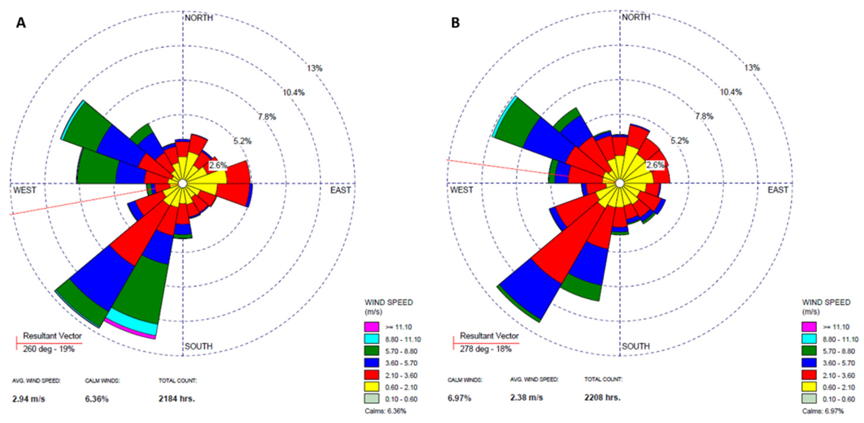
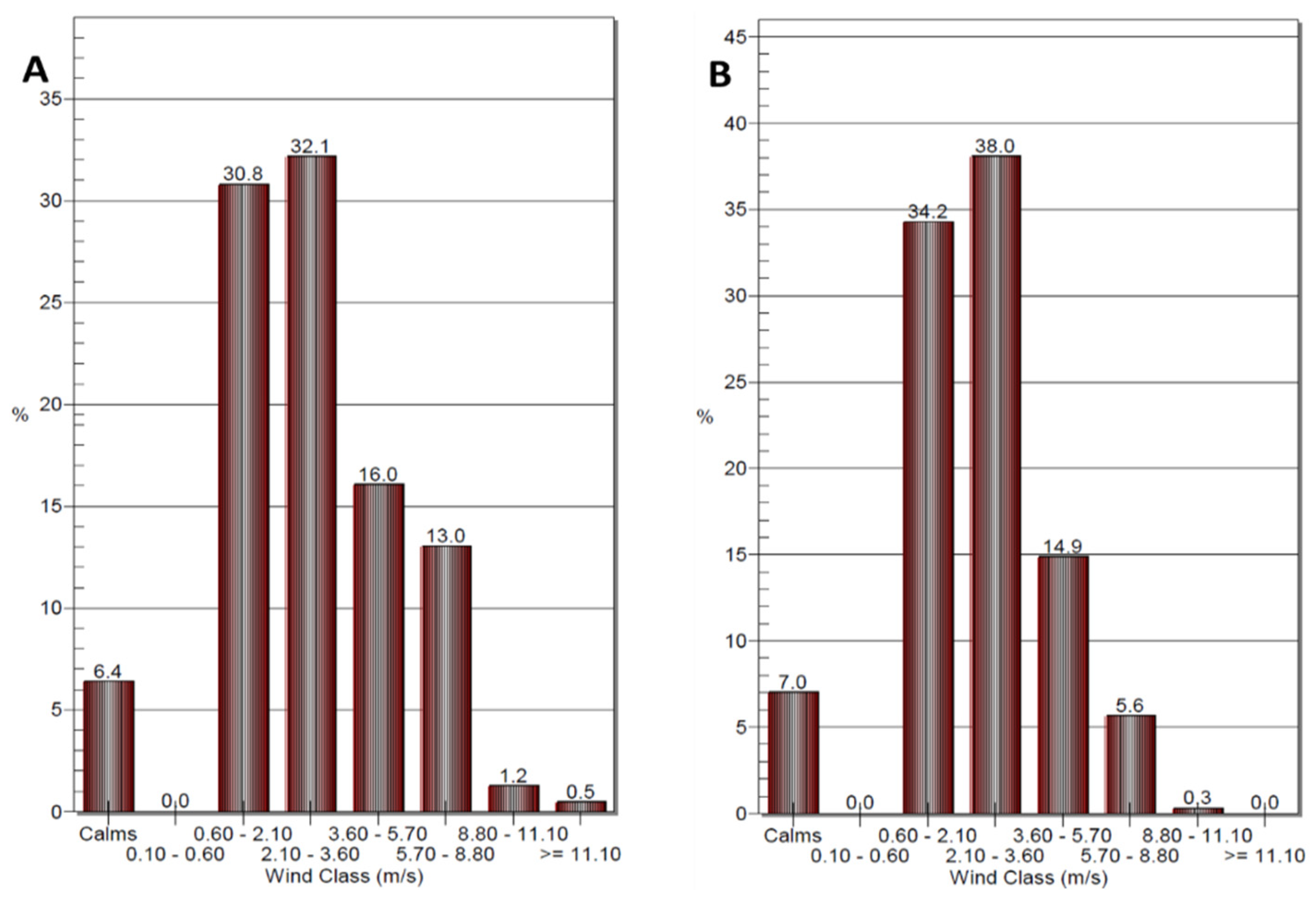
3.3. Meteorological Data Results

In general, the prevailing wind directions were observed to be from W-NW and SW (Figure 6). The wind reached speeds exceeding 11.1 m/s from the SW direction during autumn 2023, while in the second monitoring period, wind speeds ranged between 8.8 m/s and 11.1 m/s from the NW direction. However, the forest located to the west acts as a natural barrier, limiting dispersion in this direction by reducing wind speed.

Regarding the wind frequency during the autumn period of 2023, a strong presence of wind classes in the 0.6–2.1 m/s range was observed, covering approximately 30.8% of the period, with wind speeds of 2.1–3.6 m/s and 3.6–5.7 m/s covering 32.1% and 16%, respectively, of the period (Figure 7A). Winds with higher intensities in the 5.7–8.8 m/s range were observed in about 13% of the year. The average speed throughout the entire monitored period was 2.94 m/s, with the percentage of calm hours being approximately 6.36% of the year (Figure 7A).

Regarding the summer period of 2023, a strong presence of wind classes in the 0.6–2.1 m/s range was observed, covering approximately 34.2% of this period, slightly higher compared to the previous one. The following wind classes, 2.1–3.6 m/s and 3.6–5.7 m/s, cover 38% and 14.9%, respectively, of the period (Figure 7B). Winds with higher intensities in the 5.7–8.8 m/s range were observed in about 5.6% of the year. The average speed during the entire monitored period was 2.38 m/s, with calm hours accounting for approximately 6.97% of the year (Figure 7B).

The most unfavorable meteorological conditions consist of a stable atmosphere (classes E and F), low wind speeds, thermal inversions, and reduced turbulence. These conditions frequently occur at night and limit pollutant dispersion, promoting their accumulation near the source, especially in low-lying or enclosed terrain.

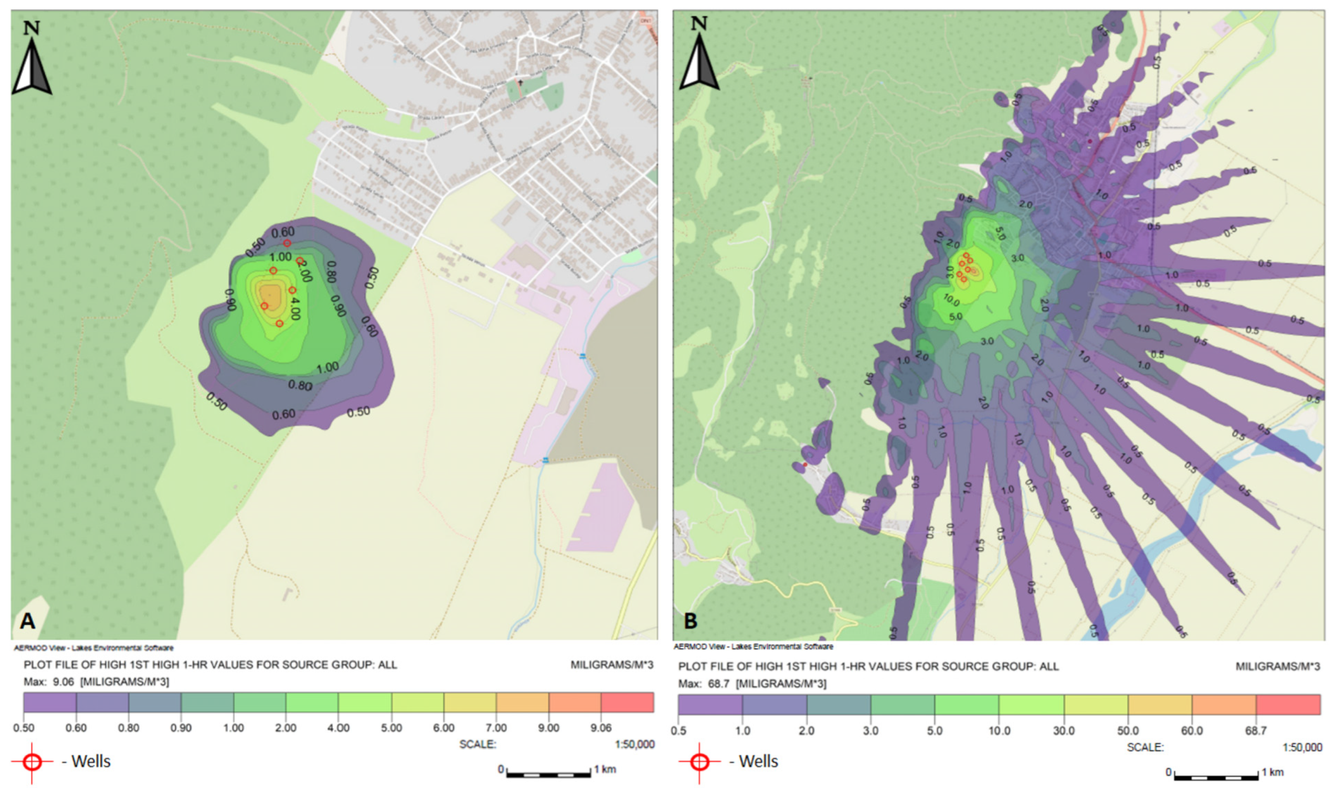
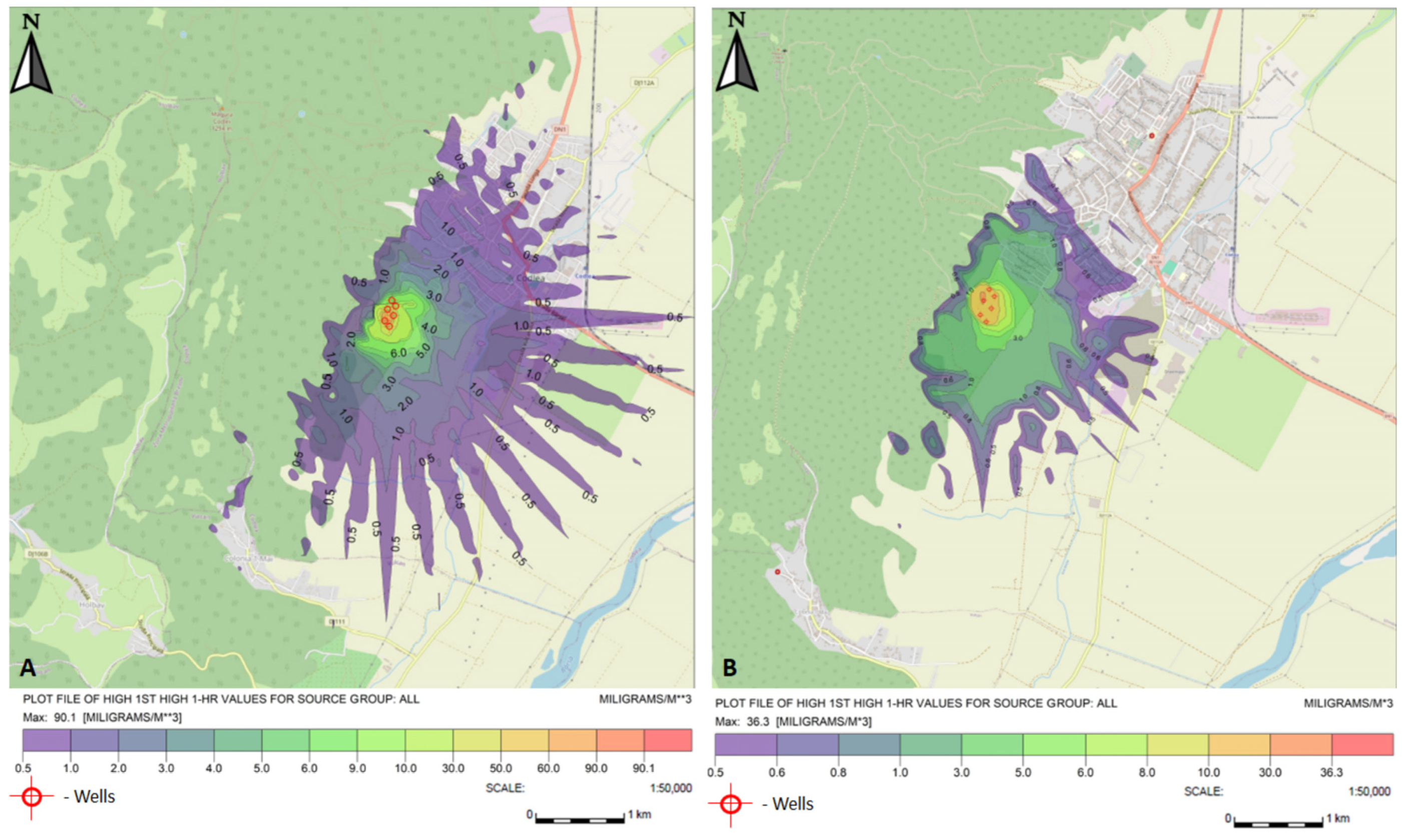
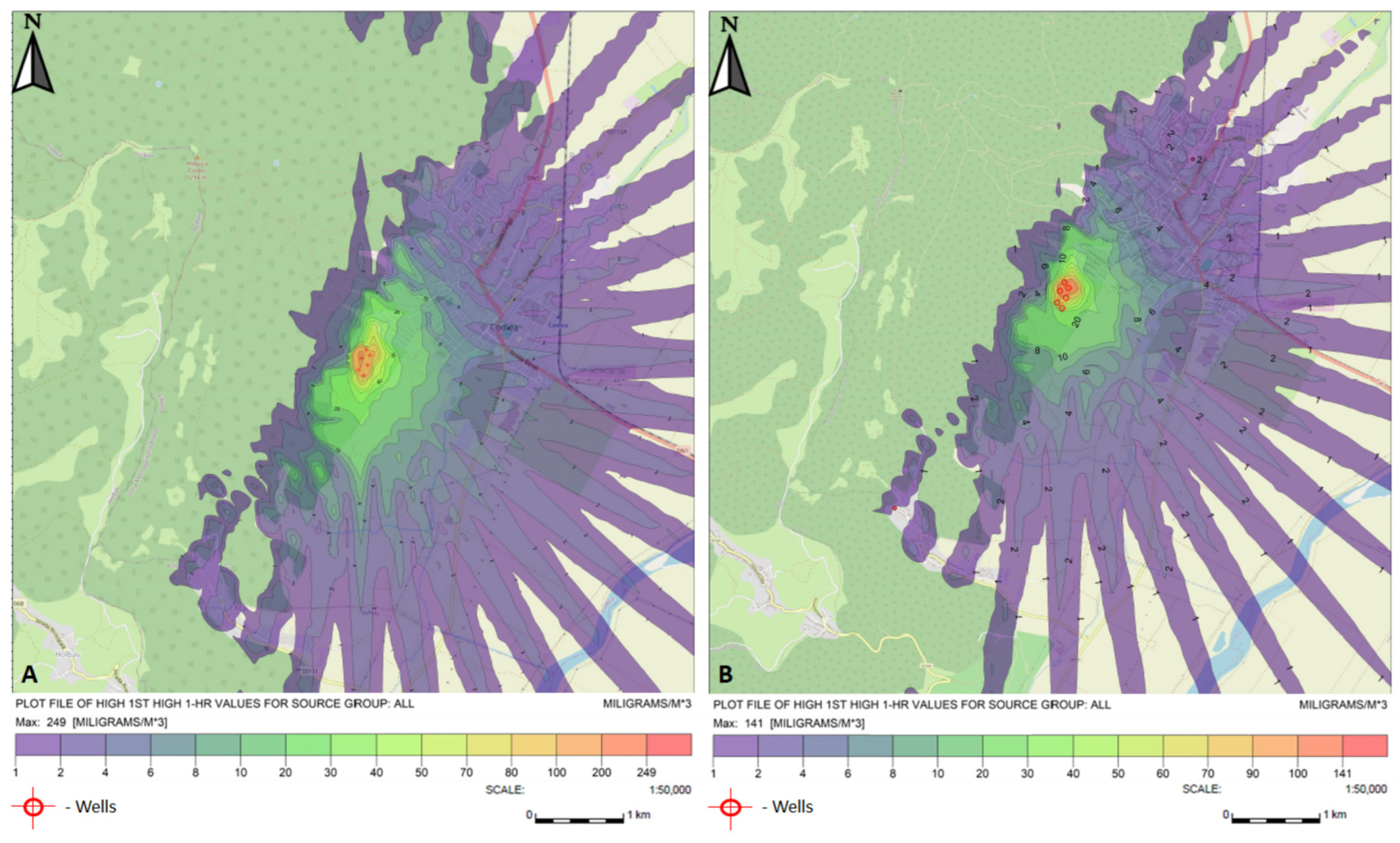
3.4. CH₄ and CO₂ Dispersion Modeling

Air dispersion modeling was performed to assess the highest ground-level concentrations of CH₄ and CO₂ gases released from P1-P6 wells. In addition, the spread of CH₄ and CO₂ emissions was studied.

In the images, the terrain is represented by different shades of green, which suggest distinct types of land cover. Typically, dark green indicates areas covered with dense vegetation, such as forests or wooded areas, while light green corresponds to agricultural land, grasslands or semi-urban areas. These distinctions are important because topography and the type of land cover can directly influence the dispersion of gases—dense vegetation can act as a barrier that slows or redirects air flows, while open land allows for faster and more uniform dispersion.

The colors used in dispersion maps are intended to visually represent variations in the concentration of a pollutant (in this case, methane and carbon dioxide) over a given area. In general, the color palette was chosen to be intuitive and easy to interpret: dark colors (such as green) indicate low values, and light colors (such as yellow, orange and red) signal high concentrations.

In the map, access roads are marked in yellow, highlighting the main transportation network in the area, while watercourses are represented in blue, indicating the presents of rivers or canals.

During the autumn season (Figure 9A), CH₄ disperses both horizontally and vertically, predominantly in the north, west, and south directions. The observed scattering pattern exhibits a radial distribution, similar to the sun’s rays, which suggests a significant influence of both wind patterns and local terrain characteristics (Figure 9B).

As seen in Figure 9, the maximum concentrations of CH₄ emissions for the autumn season in 2023 and 2024 were 9.06 mg/m³ and 68.7 mg/m³, respectively.

The hourly distribution of CH₄ concentrations during the autumn season in Figure 8 shows a relatively low dispersion rate of CH₄, covering maximum distances ranging between 0.5 and 4.6 km in the northeast and northwest directions.

During the summer, the CH₄ dispersion follows a radial pattern, maintaining its characteristics, as seen in Figure 10A. As shown in Figure 10A,B, the maximum concentrations of CH₄ in 2023 and 2024 were 90.1 mg/m³ and 36.3 mg/m³, respectively. The hourly distribution of CH₄ concentrations during the summer period, presented in Figure 9, shows a relatively low dispersion rate of the gas, with maximum spread distances ranging between 2 and 3 km in the northeast and northwest directions. Consequently, residential areas located in the north and northeast directions were exposed to CH₄ concentrations of approximately 0.5 mg/m³ to 1 mg/m³ during summer.

The simulation for CO₂ dispersion (Figure 11A) indicated a maximum concentration of 80.2 mg/m³ in the NE and SE areas of the site, under the most unfavorable meteorological conditions. At the southern part of the site boundary, the highest concentration of CO₂ recorded was 20 mg/m³. The concentrations gradually decreased, reaching values between 1 mg/m³ and 0.5 mg/m³ at distances greater than 5 km from the site.

The simulation showed in Figure 11B for all emission sources indicated a maximum concentration of 103 mg/m³, recorded on-site. The dispersion of the pollutant was lower compared to the simulation from Figure 11A, with lower isoconcentration curve values towards the east. The concentrations at the level of sensitive receptors ranged between 1 mg/m³ and 2 mg/m³.

The simulation in Figure 12A highlights a maximum concentration of 249 mg/m³ in the NE and SE regions of the site, under the most unfavorable meteorological conditions for pollutant dispersion throughout the entire study period. At the site boundary, the highest concentration of carbon dioxide reaches 40 mg/m³ in the SE part of the site. Concentrations gradually decrease as the distance from the emission source increases, reaching values between 1 mg/m³ and 2 mg/m³ at distances greater than 4.8 km from the site.

The simulation in Figure 12B, which considers all emission sources, indicates a maximum concentration of 141 mg/m³ on-site. At the level of sensitive receptors, the concentrations range between 1 mg/m³ and 4 mg/m³ in the NE direction.

The concentrations of CH₄ and CO₂ varied depending on the season, being influenced by changes in weather conditions.

4. Discussion

The AERMOD dispersion model was applied using a worst-case scenario. Although this method supports a protective assessment, it may lead to potential overestimation, particularly since such extreme atmospheric conditions occur relatively rarely. Importantly, the study did not include alternative modeling scenarios, such as the 98th percentile or average-case simulations, because the concentrations predicted under worst-case assumptions were already within an acceptable range for environmental and health protection.

Specifically, the modeled ground-level concentrations ranged from 9 mg/m³ to 249 mg/m³, depending on source parameters and meteorological conditions. These results were found to be below any thresholds of regulatory concern, especially since CH₄ and CO₂ do not have established ambient air quality limits [48]. These gases are regulated in the context of climate policy rather than as air quality pollutants.

The novelty of the study lies in the application of the AERMOD dispersion model using a worst-case scenario approach, combined with real, seasonally correlated measurements, providing a detailed understanding of how CH₄ and CO₂ concentrations vary according to meteorological conditions and terrain features. Furthermore, the methodology proposed is reproducible and can be applied to other urban and peri-urban areas with similar profiles, thus supporting the development of data-driven local environmental policies.

The study indicates that residential areas situated near the municipal waste landfill are exposed to higher concentrations of carbon dioxide compared to methane, even if the landfill is closed and covered with vegetation. The finding suggests that wind direction and speed and atmospheric stability (stable, neutral, and unstable) are the most important factors for air pollutant dispersion, as mentioned in other studies, such as the research conducted in the State of Kuwait, published in the year 2021 [7]. In addition, factors such as local topography, atmospheric reactions, and anthropogenic influences significantly contribute to the way gases spread and accumulate in the surrounding environment [7]. The dispersion of CO₂ and CH₄ also depends on a combination of physical meteorology (for example, temperature and thermal inversion and humidity and precipitation) and topography (surface type), chemical (atmospheric reactions and oxidation of CH₄ and absorption by ecosystems), and anthropogenic (emission sources) factors.

Comparing CH₄ and CO₂ concentration values obtained in our study with historical or reference datasets reveals remarkable differences that highlight the specific and intense nature of the analyzed source, biogas capture wells at a waste landfill. For methane, the reference data show concentrations ranging approximately from 1.25 mg/m³ to 25.65 mg/m³, with an estimated average around 6–8 mg/m³, reflecting typical ambient air levels in areas without major point sources [49]. In contrast, our simulations revealed much higher concentrations, ranging from 656.036 mg/m³ up to 93,616.3372 mg/m³, with even the lowest values exceeding the highest historical concentrations by several tens or hundreds of times.

A similar situation is observed for carbon dioxide. Studies from 1997 to 1999 reported values between 216 and 487 mg/m³, with an average around 270–280 mg/m³, characteristic of urban or peri-urban ambient air [49]. In our study, CO₂ concentrations varied between 2160 and 286,021 mg/m³, with an estimated average exceeding 80,000 mg/m³; these differences are explained by the nature of the source, i.e., biogas capture wells producing concentrated point emissions, unlike the diffuse or ambient sources in previous studies.

The use of advanced dispersion models such as AERMOD allowed us to simulate maximum concentrations under specific meteorological conditions. The simulations showed that in the autumn season, maximum methane concentrations reached 68.7 mg/m³, dispersing radially up to 4.6 km, affecting areas mainly in the northeast and northwest directions. During summer, maximum concentrations reached 90.1 mg/m³, with a more limited dispersion but still exposing residential areas in the north and northeast to concentrations between 0.5 and 1 mg/m³. For carbon dioxide, maximum concentrations ranged between 80.2 mg/m³ and 249 mg/m³ at the site, while concentrations in nearby residential areas 4–5 km away ranged from 1 to 4 mg/m³.

These results emphasize the importance of continuous and rigorous monitoring of biogas emissions to ensure effective air quality management and to support informed decisions regarding environmental protection and the health of communities living near the landfill site.

In a study by Mainheim et al. [14] published in 2021 regarding gas emissions from MSW landfills, Europe contributes approximately 48% of the global methane flow. The largest contributions are those of Italy (19%), Germany (13%), France (7%), Sweden (5%), with Romania contributing less than 1% [14].

Data provided by European Environment Agency highlights significant differences between European countries in terms of municipal waste landfill rates, in relation to the EU target for 2035 (a maximum of 10%). While countries in Western and Northern Europe, such as Belgium, Germany, the Netherlands, and Sweden, have already met this target, Romania is among the countries with the highest landfill rates, alongside Malta and Greece, according to data published by the EEA in December 2024 [50]. Although Romania has seen a slight decrease in the proportion of landfilled waste—from over 90% in 2010 to approximately 75% in 2022—progress remains insufficient [51]. This stagnation indicates a lack of effective waste management policies and underlines the urgent need for investments in sorting and recycling infrastructure, as well as firm legislative measures to reduce reliance on landfilling and align the country with the EU’s circular economy objectives [52]. Similar problems were reported in other European countries, such as Slovakia, based on data published by Tokarcikova E. et al. in 2024 [52].

According to statistics provided by Eurostat, in 2023, the amount of municipal waste generated per person in the European Union was 511 kg, 4 kg less than in 2022 (515 kg) and 23 kg less than in 2021 (534 kg), representing a 4.3% decrease over two years. Compared to 2013, the amount increased by 32 kg (Eurostat, 2025) [53].

The available data shows significant differences between EU member states. The highest amounts of municipal waste per person were generated in Austria (803 kg/person, 2022), Denmark (802 kg, 2022), and Luxembourg (712 kg). The lowest amounts were recorded in Romania (303 kg, 2022), Poland (367 kg), and Estonia (373 kg).

On average, 246 kg of waste per person was recycled in the EU in 2023. This means that 48.0% of the total municipal waste generated was recycled, compared to 37.2% in 2013 (199 kg/person) [34]. In 2023, 129 kg/person was incinerated (25.2% of total waste), while 115 kg/person was landfilled (22.5%). In 2013, the amount incinerated was 127 kg/person (26.4%), and the amount landfilled was 142 kg/person (29.7%) [53].

Data provided by EuroStat highlights the amount of municipal waste generated per capita in 2013 and 2023 for each EU country (and several countries outside the EU). Romania ranks last in terms of municipal waste generated per capita, both in 2013 and in 2023, with a value of approximately 300 kg/person in 2023. This is significantly below the EU average, which stood at 511 kg/person in 2023. Compared to Western European countries, the differences are substantial. Even compared to other Central and Eastern European countries, Romania generates considerably less waste [53].

However, the analyzed data reveal major challenges for Romania in the field of municipal waste management. Although the country generates the lowest amount of municipal waste per capita in the European Union (approximately 303 kg/person in 2022, compared to the EU average of 511 kg), an alarmingly high proportion of this waste continues to be landfilled: approximately 75% in 2022, a modest decrease from over 90% in 2010. This situation places Romania among the worst-performing member states, alongside Malta and Greece, in terms of meeting the EU’s 2035 target of a maximum 10% landfill rate.

The differences compared to Western and Northern European countries, which have already achieved this target, are significant and highlight the urgent need for reform. Romania must quickly invest in separate collection infrastructure, sorting, and recycling, implement strong policies and legislative measures, and promote a model based on the circular economy. Without these efforts, the risk of the country falling behind other member states is considerable, with negative impacts on both the environment and public health.

5. Conclusions

Firstly, the air dispersion modeling highlighted significant seasonal variations in the concentrations of methane (CH₄) and carbon dioxide (CO₂), depending on meteorological conditions. Thus, during the autumn season, maximum methane concentrations of up to 68.7 mg/m³ were recorded, with dispersion distances reaching up to 4.6 km, especially in the northeast and northwest directions. In the summer season, the dispersion was more limited, but the maximum CH₄ concentrations reached 90.1 mg/m³, exposing residential areas in the north and northeast to values between 0.5 and 1 mg/m³. As for CO₂, the maximum concentrations recorded in simulations ranged between 80.2 mg/m³ and 249 mg/m³ at the site, while in the vicinity of the study area (4–5 km distance), values ranged between 1 and 4 mg/m³.

Secondly, the results confirmed the decisive influence of meteorological factors (wind direction and speed, atmospheric stability) and local terrain characteristics on pollutant behavior. The observed radial dispersion and the barrier effect of the forest to the west of the site emphasize the importance of considering geographic and climatic particularities in environmental assessments. Additionally, the application of the AERMOD model enabled an accurate estimation of the spatial distribution of emissions, providing a valuable tool for predictive analysis.

In conclusion, the study significantly contributes to understanding the dispersion processes of gases originating from biogas capture wells and highlights the need for a continuous monitoring system adapted to local conditions. Furthermore, the results support the necessity of implementing effective waste management and emission control measures, in the context of climate goals and public health protection.

These findings not only reflect the complexity of interactions between emission sources and atmospheric conditions but also highlight the need for the implementation of efficient waste management strategies to minimize the risks associated with air pollution in urban and peri-urban areas. Essentially, a deep understanding of these dynamics is crucial for protecting the quality of life and developing sustainable environmental policies.

References

1. IPPC. AR6 Synthesis Report: Climate Change 2023. Available online: https://www.ipcc.ch/report/sixth-assessment-report-cycle/ (accessed on 22 May 2025).
2. UNEP. Annual Report 2023. Available online: https://www.unep.org/resources/annual-report-2023 (accessed on 22 May 2025).
3. Giordano, C.R.; Van Brunt, M.E.; Halevi, S.J.; Castaldi, M.J.; Orlovits, Z.; Illes, Z. Landfill gas collection efficiency: Categorization of data from existing in-situ measurements. Waste Manag. 2024, 175, 83–91. [Google Scholar] [CrossRef] [PubMed]
4. Yeşiller, N.; Hanson, J.L.; Manheim, D.C.; Newman, S.; Guha, A. Assessment of methane emissions from a California landfill using concurrent experimental, inventory, and modeling approaches. Waste Manag. 2022, 154, 146–159. [Google Scholar] [CrossRef]
5. Prebilic, V.; Moze, M.; Golobic, I. Waste-to-Energy Processes as a Municipality-Level Waste Management Strategy: A Case Study of Kočevje, Slovenia. Processes 2024, 12, 1010. [Google Scholar] [CrossRef]
6. Delgado, M.; López, A.; Esteban, A.L.; Lobo, A. Some findings on the spatial and temporal distribution of methane emissions in landfills. J. Clean. Prod. 2022, 362, 132334. [Google Scholar] [CrossRef]
7. Elmi, A.; Al-Harbi, M.; Yassin, M.F.; Al-Awadhi, M.M. Modeling gaseous emissions and dispersion of two major greenhouse gases from landfill sites in arid hot environment. Environ. Sci. Pollut. Res. 2021, 28, 15424–15434. [Google Scholar] [CrossRef]
8. Popli, K.; Lim, J.; Kim, H.K.; Kim, Y.M.; Tuu, N.T.; Kim, S. Prediction of greenhouse gas emission from municipal solid waste for South Korea. Environ. Eng. Res. 2020, 25, 462–469. [Google Scholar] [CrossRef]
9. Kaza, S.; Yao, L.C.; Bhada-Tata, P.; Van Woerden, F. What a Waste 2.0: A Global Snapshot of Solid Waste Management to 2050; World Bank: Washington, DC, USA, 2018; Available online: https://openknowledge.worldbank.org/handle/10986/30317 (accessed on 2 April 2025).
10. Mor, S.; Ravindra, K. Municipal solid waste landfills in lower- and middle-income countries: Environmental impacts, challenges and sustainable management practices. Process Saf. Environ. Prot. 2023, 174, 510–530. [Google Scholar] [CrossRef]
11. Khafagy, S.M.N.M.; Sarmmak, A.E.; Emara, K. Modeling of methane emissions from waste disposal sites at selected Egyptian governorates and potential energy production from waste-to-energy projects. Sci. Rep. 2024, 14, 25040. [Google Scholar] [CrossRef]
12. Zambrano-Monserrate, M.A.; Ruano, M.A.; Ormeño-Candelario, V. Determinants of municipal solid waste: A global analysis by countries’ income level. Environ. Sci. Pollut. Res. 2021, 28, 62421–62430. [Google Scholar] [CrossRef]
13. Przydatek, G.; Generowicz, A.; Kanownik, W. Evaluation of the Activity of a Municipal Waste Landfill Site in the Operational and Non-Operational Sectors Based on Landfill Gas Productivity. Energies 2024, 17, 2421. [Google Scholar] [CrossRef]
14. Manheim, D.C.; Yeşiller, N.; Hanson, J.L. Gas Emissions from Municipal Solid Waste Landfills: A Comprehensive Review and Analysis of Global Data. J. Indian Inst. Sci. 2021, 101, 625–657. [Google Scholar] [CrossRef]
15. Manea, E.E.; Bumbac, C.; Dinu, L.R.; Bumbac, M.; Nicolescu, C.M. Composting as a sustainable solution for organic solid waste management: Current practices and potential improvements. Sustainability 2024, 16, 6329. [Google Scholar] [CrossRef]
16. Duan, Z.; Scheutz, C.; Kjeldsen, P. Trace gas emissions from municipal solid waste landfills: A review. Waste Manag. 2021, 119, 39–62. [Google Scholar] [CrossRef]
17. Molodtsov, D.V.; Mikheev, P.Y.; Maslikov, V.I. Assessment of the possibility of obtaining biohydrogen during decarbonization of municipal solid waste landfills. Int. J. Hydrogen Energy 2024, 82, 853–857. [Google Scholar] [CrossRef]
18. Mønster, J.; Kjeldsen, P.; Scheutz, C. Methodologies for measuring fugitive methane emissions from landfills—A review. Waste Manag. 2019, 87, 835–859. [Google Scholar] [CrossRef]
19. Yilmaz, M.; Tinjum, J.M.; Acker, C.; Marten, B. Transport mechanisms and emission of landfill gas through various cover soil configurations in an MSW landfill using a static flux chamber technique. J. Environ. Manag. 2021, 280, 111677. [Google Scholar] [CrossRef]
20. Khanal, S.K. Anaerobic Biotechnology for Bioenergy Production. Principles and Application; Willey-Blackwell Publishing: Oxford, UK, 2008; pp. 29–41. [Google Scholar] [CrossRef]
21. McBain, M.C.; Warland, J.S.; McBride, R.A.; Wagner-Riddle, C. Micrometeorological measurements of N2O and CH4 emissions from a municipal solid waste landfill. Waste Manag. Res. 2005, 23, 409–419. [Google Scholar] [CrossRef]
22. Chetri, J.K.; Reddy, K.R. Advancements in Municipal Solid Waste Landfill Cover System: A Review. J. Indian Inst. Sci. 2021, 101, 557–588. [Google Scholar] [CrossRef]
23. Delgado, M.; López, A.; Esteban-García, A.L.; Lobo, A. The importance of particularizing the model to estimate landfill GHG emissions. J. Environ. Manag. 2023, 325, 116600. [Google Scholar] [CrossRef] [PubMed]
24. Ren, Y.; Zhang, Z.; Huang, M. A review on settlement models of municipal. Waste Manag. 2022, 149, 79–95. [Google Scholar] [CrossRef] [PubMed]
25. IPCC. Methodology Report. Good Practice Guidance and Uncertainty Management in National Greenhouse Gas Inventories. 2000. Available online: https://www.ipcc.ch/publication/good-practice-guidance-and-uncertainty-management-in-national-greenhouse-gas-inventories/ (accessed on 27 May 2025).
26. Tadesse, A.; Lee, J. Utilization of methane from municipal solid waste landfills. Environ. Eng. Res. 2024, 29, 230166. [Google Scholar] [CrossRef]
27. US EPA. Importance of Methane. Available online: https://www.epa.gov/gmi/importance-methane?utm (accessed on 22 May 2025).
28. Lombardi, M.; Mauri, F.; Fargnoli, M.; Napoleoni, Q.; Berardi, D.; Berardi, S. Occupational Risk Assessment in Landfills: Research Outcomes from Italy. Safety 2023, 9, 3. [Google Scholar] [CrossRef]
29. Scarpelli, T.R.; Cusworth, D.H.; Duren, R.M.; Kim, J.; Heckler, J.; Asner, G.P.; Thoma, E.; Krause, M.J.; Heins, D.; Thorneloe, S. Investigating Major Sources of Methane Emissions at US Landfills. Environ. Sci. Technol. 2024, 58, 21545–21556. [Google Scholar] [CrossRef] [PubMed]
30. US EPA. National Enforcement and Compliance Initiatives (NECIs) for Fiscal Years 2024−2027. 2023. Available online: https://www.epa.gov/enforcement/national-enforcement-and-compliance-initiatives (accessed on 29 May 2025).
31. US EPA. Quantifying Methane Emissions from Landfilled Food Waste. 2023. Available online: https://www.epa.gov/land-research/quantifying-methane-emissions-landfilled-food-waste (accessed on 29 May 2025).
32. Imbiribaa, B.C.O.; Ramosa, J.R.S.; de Sousa Silva, R.; Cattanioa, J.H.; do Coutod, L.L.; Mitschein, T.A. Estimates of methane emissions and comparison with gas mass burned in CDM action in a large landfill in Eastern Amazon. Waste Manag. 2020, 101, 28–34. [Google Scholar] [CrossRef]
33. Kamalan, H. A new empirical model to estimate landfill gas pollution. J. Health Sci. Surveill. Syst. 2016, 4, 142–148. [Google Scholar]
34. Ali, M.; Zhang, J.; Raga, R.; Lavagnolo, M.C.; Pivato, A.; Wang, X.; Zhang, Y.; Cossu, R.; Yue, D. Effectiveness of aerobic pretreatment of municipal solid waste for accelerating biogas generation during simulated landfilling. Front. Environ. Sci. Eng. 2018, 12, 5. [Google Scholar] [CrossRef]
35. Folino, A.; Gentili, E.; Komilis, D.; Calabrò, P.S. Biogas recovery from a state-of-the-art Italian landfill. J. Environ. Manag. 2024, 367, 122040. [Google Scholar] [CrossRef] [PubMed]
36. Jiang, G.; Liu, D.; Chen, W.; Han, Z.; Li, Q. Greenhouse gas emissions from semi-aerobic bioreactor landfills with different vent-pipe diameters. Environ. Sci. Pollut. Res. 2021, 28, 17563–17572. [Google Scholar] [CrossRef]
37. BP, N.; Tabaroei, A.; Garg, A. Methane Emission and Carbon Sequestration Potential from Municipal Solid Waste Landfill, India. Sustainability 2023, 15, 7125. [Google Scholar] [CrossRef]
38. Balasus, N.; Jacob, D.J.; Maxemin, G.; Jenks, C.; Nesser, H.; Maasakkers, J.D.; Cusworth, D.H.; Scarpelli, T.R.; Varon, D.J.; Wang, X. Satellite monitoring of annual US landfill methane emissions and trends. Environ. Res. Lett. 2025, 20, 024007. [Google Scholar] [CrossRef]
39. Xu, J.; Liu, Z.; Dai, J. Environmental and economic trade-off-based approaches towards urban household waste and crop straw disposal for biogas power generation project -a case study from China. J. Clean. Prod. 2021, 319, 128620. [Google Scholar] [CrossRef]
40. Jacob, R.; Sergeev, D.; Muller, M. Valorisation of waste materials for high temperature thermal storage: A review. J. Energy Storage 2022, 47, 103645. [Google Scholar] [CrossRef]
41. Zhazhkov, V.V.; Politaeva, N.A.; Velnozhina, K.A.; Shinkovich, P.S.; Norov, B.K. Production of biogas from organic waste at landfills by anaerobic digestion and its further conversion into biohydrogen. Int. J. Hydrogen Energy 2024, 70, 779–785. [Google Scholar] [CrossRef]
42. European Environmental Agency. Available online: https://www.eea.europa.eu/publications/many-eu-member-states/romania/view (accessed on 4 April 2025).
43. Government Ordinance No. 2 of August 11, 2021, Regarding Waste Disposal. Available online: https://legislatie.just.ro/Public/DetaliiDocumentAfis/245381 (accessed on 31 July 2024). (In Romanian).
44. Technical Norm of November 26, 2004, on Waste Disposal. Available online: https://legislatie.just.ro/Public/DetaliiDocument/200022 (accessed on 31 July 2024). (In Romanian).
45. U.S. Environmental Protection Agency. AERMOD Implementation Guide. 2021. Available online: https://nepis.epa.gov/ (accessed on 30 May 2025).
46. Optima Biogas. Available online: www.mru.eu (accessed on 25 March 2025).
47. Romanian National Meteorological Administration. Available online: https://www.meteoromania.ro/ (accessed on 31 July 2024). (In Romanian).
48. Directive 2008/50/CE Transpose in Romanian Legislation by Law No. 104/2011 Regarding Air Quality. Available online: https://calitateaer.ro/public/legislation-page/national-legislation-page/?__locale=en (accessed on 2 April 2025). (In Romanian).
49. Hegde, U.; Chang, T.C.; Yang, S.S. Methane and carbon dioxide emissions from Shan-Chu-Ku landfill site in northern Taiwan. Chemosphere 2003, 52, 1275–1285. [Google Scholar] [CrossRef] [PubMed]
50. European Environment Agency. Available online: https://www.eea.europa.eu/en/analysis/indicators/diversion-of-waste-from-landfill (accessed on 15 April 2025).
51. Iacoboaea, C.; Luca, O.; Petrescu, F. An analysis of Romania’s municipal waste within the European context. Theor. Empir. Res. Urban Manag. 2013, 8, 73–84. [Google Scholar]
52. Tokarcikova, E.; Durisova, M.; Trojakova, T. Circular Economy: Municipal solid waste and landfilling analyses in Slovakia. Economies 2024, 12, 289. [Google Scholar] [CrossRef]
53. EuroStat. Available online: https://ec.europa.eu/eurostat/web/products-eurostat-news/w/ddn-20250213-1 (accessed on 16 April 2025).
Figure 1. Gas composition % by volume in different phases of waste decomposition in landfill sites [10], copyright from Elsevier.
Atmosphere 16 00752 g001
Figure 2. Process flow diagram for storage, leachate treatment, and biogas capture.
Atmosphere 16 00752 g002
Figure 3. The localization of points where sensitive receptors were introduced.
Atmosphere 16 00752 g003
Figure 4. Images from the site of a municipal solid waste storage station (A); the measurement of CH4 and CO2 from the biogas capture well (B).
Atmosphere 16 00752 g004
Figure 5. Methodology applied.
Atmosphere 16 00752 g005
Figure 6. Hourly wind direction and speed data (wind rose) for autumn season 2023 (A), and summer season 2023 (B).
Atmosphere 16 00752 g006
Figure 7. The distribution of wind speed frequency by class for autumn season 2023 (A) and during summer season 2023 (B).
Atmosphere 16 00752 g007
Figure 8. Mean values and related standard deviations of CH4 (A) and CO2 (B) concentrations during the investigated period at the level of sensitive receptors (different letters indicate significant differences).
Atmosphere 16 00752 g008
Figure 9. Distribution of the CH4 concentrations during autumn season 2023 (A), and autumn season 2024 (B).
Atmosphere 16 00752 g009
Figure 10. Distribution of the CH4 concentrations during summer season 2023 (A), and summer season 2024 (B).
Atmosphere 16 00752 g010
Figure 11. Distribution of the CO2 concentrations during autumn season 2023 (A), and autumn season 2024 (B).
Atmosphere 16 00752 g011
Figure 12. Distribution of the CO2 concentrations during summer season 2023 (A), and summer season 2024 (B).
Atmosphere 16 00752 g012