1. Introduction
Meteorological disasters induced by severe convective weather represent one of China’s most devastating natural hazards. Dominated by meso- and micro-scale convective systems, such weather exhibits pronounced spatial heterogeneity [
1]. Typical severe convective processes include short-duration heavy rainfall, thunderstorms, gales, hail, tornadoes, and squall lines. These hazards fundamentally arise from synergistic effects of thermodynamic instability energy, vertical wind shear, and moisture transport, characterized by localized coverage, rapid intensification, extreme convective intensity, and severe damage potential, thereby posing significant challenges for operational forecasting.
In recent years, the application of convection-allowing models (CAMs) has become a critical approach to improving the precision of severe convective weather forecasting. CAMs typically employ horizontal grid resolutions of 1–4 km, eliminating the need for cumulus parameterization schemes. By enhancing grid resolution, CAMs can better resolve detailed features of convective systems, significantly improving simulations of convective initiation mechanisms, organizational modes, and evolutionary processes [
2,
3]. Nevertheless, limitations persist in resolving small-scale convective dynamics and cloud microphysical processes, known as the “gray zone” problem [
4,
5,
6]. Furthermore, inherent errors in the initial conditions of CAMs from assimilating high spatiotemporal resolution observations constrain precise depiction of convective triggering mechanisms [
7,
8], underscoring the critical need to account for the impacts of forecast uncertainty.
Ensemble forecasting serves as an effective methodology to address model errors and initial perturbation uncertainties [
9]. By constructing optimal estimates of initial condition and model error uncertainties that align closely with actual states, it comprehensively predicts probabilistic future events. Extensive forecasting experiments confirm that convection-allowing ensemble forecasting significantly outperforms traditional deterministic forecasting in prediction skill [
10,
11,
12]. A critical challenge in convection-allaying ensemble forecasting lies in developing physically consistent initial perturbations. Current perturbation methods predominantly inherit global or regional ensemble forecasting theories, including Breeding of Growth Modes (BGM) [
13], Singular Vectors (SVs) [
14], Ensemble Transform (ET) [
15], Ensemble Transform Kalman Filter (ETKF) [
16,
17,
18,
19], and Ensemble Kalman Filter (EnKF) [
20]. However, applications to convection-allowing scales may still encounter inadequate ensemble spread, low ensemble diversity, and mismatches between lateral boundary perturbations and initial perturbations [
21,
22]. To account for nonlinear characteristics of mesoscale phenomena, Huo [
23] conducted track ensemble forecasting experiments for Typhoon Matsa (2005) using orthogonal Conditional Nonlinear Optimal Perturbation (CNOP), SVs, and hybrid CNOP+SVs approaches in the MM5 model. The study revealed that orthogonal CNOP generates perturbations with broader spatial distributions that better characterize forecast uncertainty; however, further validation is required for CNOP’s practical effectiveness in severe convective weather prediction. Internationally, enhancing spatial orthogonality of ensemble perturbations to increase effective ensemble dimensions has become a mainstream approach. Compared to rapidly growing initial error perturbation methods, this strategy demonstrates improved ensemble spread characteristics [
24,
25].
Building upon the Ensemble Transform (ET) framework, Bishop integrated Kalman filter theory to develop the Ensemble Transform Kalman Filter (ETKF) method [
16]. Wang pioneered the application of ETKF in constructing ensemble forecast initial perturbations, demonstrating enhanced predictive skills across multiple studies [
17,
18,
19]. The ETKF method features orthogonal perturbations and flow-dependent properties that enhance effective dimensional representation of perturbation directions, while explicitly accounting for observational uncertainty impacts on initial conditions. Zhang et al. [
26] advanced ETKF implementation in the GRAPES regional ensemble prediction system by incorporating real radiosonde observations to characterize observational uncertainties. Their design of a novel initial perturbation amplitude adjustment factor improved perturbation stability and substantially enhanced precipitation prediction skills. Wang et al. [
27] investigated ETKF-derived initial perturbation structures and growth characteristics in the GRAPES-REPS system, revealing that while ensemble forecasts could capture error structures, inherent spread deficiency persisted. Their findings suggested that increasing ensemble member resolution could amplify large-scale perturbation wave energy in mid-upper atmospheric layers. Wang et al. [
28] developed an innovative analysis-constrained perturbation approach that integrates data assimilation increments into ETKF. This method enables initial perturbations to align more closely with forecast error structures and amplitudes across different spatial scales. Since its introduction to the GRAPES regional ensemble system in 2014 [
29], the optimization and refinement of ETKF initial perturbations have remained focal research topics in China’s ensemble prediction community.
An alternative initial perturbation methodology, the classical Breeding of Growing Modes (BGM) method, effectively captures fast-growing perturbation directions in ensemble subspace errors. However, it primarily accounts for vertical inhomogeneity of perturbations while neglecting horizontal inhomogeneity considerations. To address spatial localization characteristics of perturbation growth, Chen et al. [
30] proposed the Local Breeding of Growing Modes (LBGM), which generates initial perturbations with enhanced small-scale perturbation features. Ma et al. [
31] quantified localized information characteristics of LBGM and BGM using information entropy theory, demonstrating that each LBGM breeding cycle induces a distinct information leap in localized regions. Li et al. [
32] further applied LBGM to two squall line cases and developed a Gaussian weighting-based local radius selection method to account for grid point correlation heterogeneity within localized domains. Recently, Liu et al. [
33] evaluated LBGM-EPS performance for heavy rainfall events over complex topography in southwestern China’s plateau region using object-based diagnostic evaluation (MODE). Their results revealed LBGM-EPS outperforms BGM-EPS in matching precipitation object morphology and spatial distribution.
Under the convection-allowing ensemble prediction framework, LBGM with strong spatial locality and ETKF with orthogonality represent two fundamentally distinct perturbation generation strategies. The relative advantages of their respective ensemble perturbation structures, the differences in their perturbation energy evolution characteristics, and their performance in ensemble forecasting systems remain to be explored. Based on this, this study takes a severe convective squall line event in Nanchang City, Jiangxi Province, from 30 to 31 March 2024, as a case. It employs both LBGM and ETKF methods to generate initial perturbations and conducts convection-permitting ensemble forecast experiments. The study compares the ensemble members produced by the two initial perturbations using methods such as perturbation dispersion analysis, ensemble consistency, total moisture energy, kinetic energy spectrum, and perturbation and error correlation analysis (PECA). Additionally, it evaluates the differences in the predictive capabilities of precipitation and radar reflectivity between the two methods, aiming to provide theoretical foundations and optimization pathways for advancing initial perturbation methodologies in convection-allowing ensemble prediction systems.
2. Materials and Methods
The experiment utilizes version V4.2 of the Weather Research and Forecasting (WRF) model. The background field and lateral boundary conditions are derived from the National Centers for Environmental Prediction Global Forecast System (NCEP GFS), which offers a resolution of 0.25° by 0.25°. The lateral boundary data are refreshed at six-hour intervals.
The forecasting assessment utilized hourly reanalysis data from the ERA5 dataset provided by the European Centre for Medium-Range Weather Forecasts (ECMWF), characterized by a spatial resolution of 0.25° × 0.25°. This dataset encompasses various meteorological parameters, including potential height, temperature, wind fields, and specific humidity. The observational data incorporated into the model were sourced from the National Environmental Forecasting Center (NCEP) of the United States, comprising global high-altitude and surface weather observations. These observations include land surface and ocean surface data, as well as reports from weather balloons and aircraft, which are disseminated through the Global Satellite Communications System (GTS). Additionally, the model integrates wind field data obtained from radiosondes and U.S. radar systems, as well as ocean wind and total column water (TCW) data from the Special Sensor Microwave Imager (SSM/I). Satellite-derived wind field data from the National Environmental Satellite Data and Information Administration (NESDIS) are also included, providing information on pressure, potential altitude, temperature, dew point temperature, wind direction, and wind speed at six-hour intervals. Precipitation data were analyzed using the global 0.1° × 0.1° half-hour final run satellite precipitation data from the Global Precipitation Measurement (GPM) comprehensive inversion product. Furthermore, radar reflectance images were obtained from the six-minute imagery of the SWAN 3.0 RADAMCR high-resolution radar data fusion product developed by the China Meteorological Administration.
Two distinct groups of convection-permitting ensemble forecast experiments were designed and analyzed. The initial perturbation schemes employed were the LBGM and the ETKF, designated as the LBGM and ETKF groups, respectively, with each group comprising 20 ensemble members. The forecasting period spanned from 0000 UTC 30 March to 0000 UTC 31 March 2024 (all times UTC). The model utilized a double-layer bidirectional nested configuration (refer to
Figure 1). The outer layer exhibited a horizontal resolution of 9 km, encompassing a grid of 400 × 420 points, while the inner layer, designated as the analysis area, had a horizontal resolution of 3 km, with a grid of 334 × 349 points. The vertical dimension was stratified into 35 layers at non-uniform intervals, extending to a model top of 50 hPa. All ensemble members across both experimental groups employed an identical physical parameterization scheme, as detailed in
Table 1.
The experimental framework was organized into two distinct phases: the cultivation phase (referred to as the cycle update phase for the ETKF group) and the prediction phase. The initiation of the cultivation phase for the LBGM group commenced at 1800 UTC 28 March 2024, with a disturbance adjustment interval of six hours. The variables subject to adjustment during this period included the horizontal zonal wind speed (), horizontal radial wind speed (), vertical wind speed (), potential temperature (), potential height (), and water vapor mixing ratio (). The commencement of the cyclic calculations for the ETKF group aligned with that of the LBGM group, also featuring a six-hour disturbance update interval. Following a designated period of cyclic updates aimed at enhancing the stability and rationality of the disturbance adjustments, these adjustments were subsequently considered as the initial disturbances for the ensemble members. It is important to note that the disturbance variables from the cyclic updates were incorporated into the dry air column mass disturbance, building upon the adjustments made in the LBGM framework.
2.1. Initial Value Perturbation Method
2.1.1. LBGM
The Local Breeding of Growing Modes (LBGM) incorporates modifications to the scaling coefficient within the local horizontal space, building upon the foundational principles of the original BGM algorithm. The particular adjustments pertaining to the perturbations are detailed as follows:
where
and
represent the analysis perturbation and forecast perturbation, respectively, at the horizontal grid point
on the
-th vertical level in the ensemble forecasting system.
denotes the scaling coefficient at the corresponding vertical level, which is explicitly formulated as follows:
where
denotes the differential field between the perturbation prediction and the control prediction of any physical quantity subject to perturbation at time
during the breeding period. An influence radius parameter
is introduced to determine the number of grid points included in the local space.
denotes the 6-hour forecast root-mean-square error (RMSE) at time
, and
represents the 6-hour forecast root-mean-square error (RMSE) at horizontal grid point
on vertical level
at time
.
2.1.2. ETKF
The fundamental principle of the Ensemble Transform Kalman Filter (ETKF) method lies in utilizing a transformation matrix
to convert forecast perturbations from the previous assimilation cycle into analysis perturbations for ensemble members:
In the framework of ensemble perturbation construction, let
and
represent the state vectors corresponding to the analysis and prediction perturbations of the
-th member of the ensemble, respectively.
denotes the mean value of the state vectors from
prediction perturbations, while
signifies the mean value of the state vectors from
analysis perturbations. The analysis and prediction perturbation vectors are then defined accordingly.
Then, the covariance of the analysis and prediction errors can be expressed as follows:
According to Equation (4), the covariance of the analysis error can be expressed as follows:
The Kalman filter error covariance update equation is formulated as follows:
The transformation matrix can be obtained by solving it as follows:
Among them, the column vector of matrix is the eigenvector of , and its eigenvalue is the non-zero element of the diagonal matrix . In addition, is the covariance matrix of observation error, is the observation operator, and is the identity matrix. When the covariance error matrix of the forecast disturbance vector is equal to the true forecast error covariance matrix , the covariance matrix of the transformed analysis perturbation vector will be equal to the true analysis error covariance matrix.
Meanwhile, considering that the number of ensemble members is significantly less than the number of directions of the prediction error variance, the covariance of the analysis perturbation is smaller than the true covariance of the analysis error. In Wang (2003) [
17], inflation factors were introduced to amplify the analysis perturbations. This ensures consistency between the ensemble forecast variance and the error variance at all observational sites.
The inflation factor is defined as , and is calculated by the new information vector at different times and the diagonal elements of matrix .
3. Synoptic Analysis
During the experimental period from 1200 UTC 30 March to 0000 UTC 31 March 2024, Jiangxi Province in northern China experienced a rare extreme squall line weather process, characterized primarily by severe thunderstorms, strong winds, heavy rainfall, and localized hail. The leading edge of the squall line generated a strong downdraft, which formed a downburst upon impacting the ground, resulting in straight-line winds. In some counties, the maximum wind speed reached 35.3 m/s, causing significant economic losses.
Figure 2 presents the synoptic configurations along with the distributions of water vapor flux and water vapor flux divergence at 1200 UTC 30 March 2024. Prior to the squall line entering the region, the northwest of Jiangxi Province at the 500 hPa level was under the influence of southwest airflow ahead of a short-wave trough (
Figure 2a). A high-pressure ridge in northern Sichuan guided cold air from northwestern regions into the middle troposphere of northwest Jiangxi, combining with low-level warm and moist airflow to create an unstable stratification with cold air above and warm air below. At the 850 hPa level (
Figure 2b), there was a low-level jet exceeding 16 m/s across Guangxi and Guangdong to the south of Hunan Province, with prevailing southwest airflow. A cold-type shear line was triggered in the low-level airflow in western Hunan, while a warm and moist shear line was present in northern Jiangxi. The center of the low-level vortex was located near the geometric intersection of these two shear lines, and the convergence of wind fields further enhanced vertical motion. Water vapor transport analysis (
Figure 2c) indicated that southwest airflow at low levels carried a substantial amount of water vapor, with water vapor flux exceeding 22 g/(s·cm·hPa) in eastern Guangxi. The low-level jet provided favorable conditions for the southwest warm and moist air mass to transport toward northwest Jiangxi. Based on the distribution of water vapor flux divergence (
Figure 2d), the primary water vapor accumulation area was in the northwest of Jiangxi Province, and the convergence and upward movement of low-level water vapor further intensified the occurrence of severe convective weather.
4. Analysis of Experimental Results
4.1. Root Mean Square Error and Ensemble Spread
Root mean square error (RMSE) and ensemble spread are critical metrics for evaluating system performance. RMSE quantifies the deviation between the ensemble mean forecast and observations, reflecting forecast accuracy, while spread characterizes the dispersion among ensemble members, representing forecast uncertainty.
Figure 3 illustrates the temporal evolution of RMSE, spread, and the consistency ratio (RMSE/spread) for zonal wind (
), meridional wind (
), specific humidity (
), and temperature (
) at the 500 hPa pressure level. In the mid-troposphere (500 hPa), LBGM exhibits significantly lower RMSE than ETKF, indicating superior accuracy in simulating mid-level variables—a conclusion consistent with findings at 200 hPa. At the lower troposphere (850 hPa,
Figure 4), LBGM demonstrates more pronounced RMSE improvements for temperature throughout the forecast period.
For
,
, and
T, both methods show gradual spread growth with increasing forecast lead time, followed by slight reductions in spread during later stages. However, LBGM consistently exhibits smaller spread than ETKF, likely due to inherent limitations of BGM-derived perturbation directionality. This phenomenon could be attributed to the fact that the LBGM method remains constrained by the inherent directional limitations of perturbations characteristic of the BGM framework. Through iterative mode selection and breeding processes, the fastest growing perturbations emerge with more concentrated variance directions [
17]. Consequently, although LBGM achieves RMSE advantages across variables at different levels during early forecast stages, ETKF generally exhibits higher ensemble consistency metrics owing to LBGM’s spread deficiency.
4.2. Perturbation Spread
Figure 5 and
Figure 6 further illustrate the temporal evolution of zonal wind spread at the 500 hPa and 850 hPa pressure levels for both initial perturbation methods. When the ensemble spread and its evolution align with synoptic system developments, the perturbation method demonstrates superior flow-dependent characteristics [
34], indicating perturbation growth tightly coupled with dynamical systems. A comprehensive comparison reveals that spread in dynamical fields (zonal wind
, meridional wind
) better captures the southeastward propagation of the squall line. Taking
as an example, horizontal distributions of high-spread regions in LBGM and ETKF generally reflect the squall line’s positional evolution observed in radar reflectivity. ETKF exhibits rapid spread growth with stronger mean intensity and clearer bow-shaped structural features. However, at the 18-h forecast lead time, the high-spread regions of the ETKF method are displaced southeastward relative to the observed squall line position, with an eastward bias emerging by the 21-h lead time. In the lower troposphere (850 hPa), the ETKF method exhibits a more localized spread distribution, demonstrating better positional alignment and a more pronounced amplitude increase.
In comparison, the LBGM method exhibits a more reasonable spatial distribution of spread at the 500 hPa level, with weaker intensity yet generally consistent with the positions of intense squall line radar echoes. However, at the 850 hPa level under the 18-h forecast lead time, the LBGM method demonstrates significantly lower zonal wind spread levels in the northern Jiangxi region. Collectively, while the LBGM method demonstrates superior performance in spatial coherence of dynamical field spread, it systematically underestimates the spread magnitude. This discrepancy may result from the LBGM method’s stronger emphasis on localization considerations, leading to more pronounced improvements in perturbation positioning compared to the ETKF method. In contrast, the ETKF method achieves substantial enhancement in spread intensity, particularly with marked improvements in the lower troposphere.
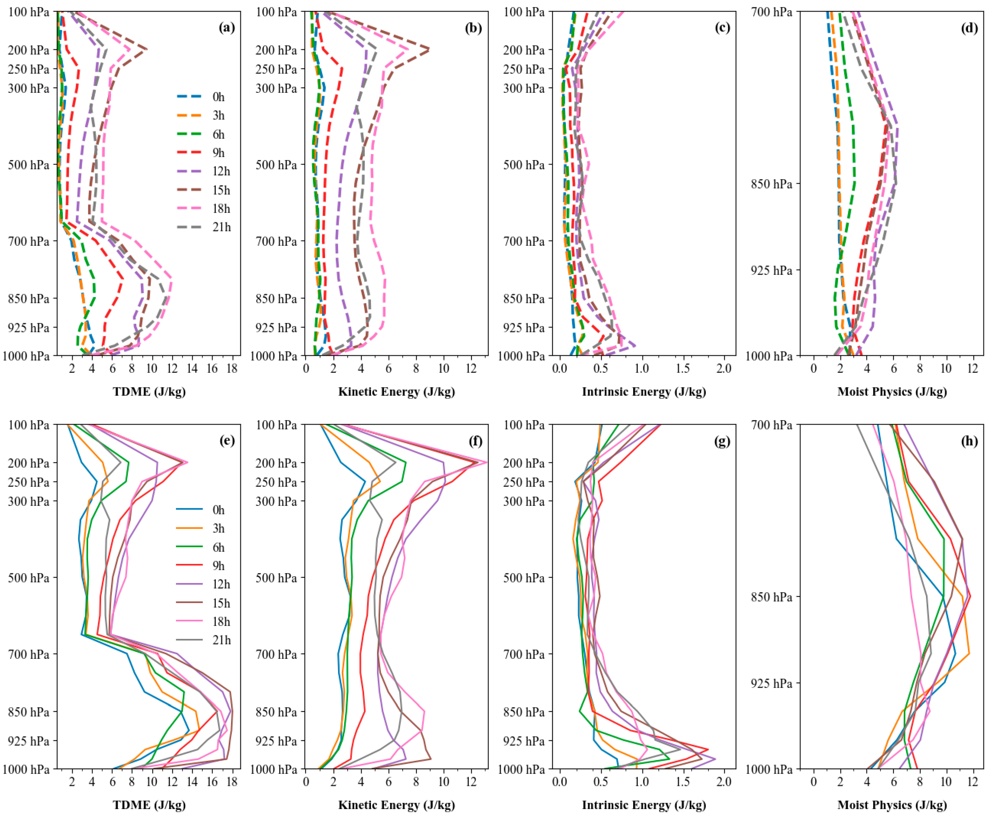
4.3. Perturbation Energy
The evolution of perturbation energy serves as a metric to evaluate the uncertainty characterization of initial perturbations and effectively captures the temporal variation of forecast errors. Perturbations in convection-allowing ensemble forecasts are primarily associated with latent heating and moist convective instability [
35], making it critical to account for the impacts of moist convective processes. To diagnose the temporal evolution characteristics of initial perturbation structures across different vertical levels, the total moist energy (TDME) is adopted as a diagnostic metric [
36,
37]. The TDME formula is expressed as follows:
In the formula, , and represent the horizontal wind perturbations, temperature perturbations, specific humidity perturbations, and surface pressure perturbations, respectively. The indices , and denote horizontal and vertical grid points. denotes the specific heat capacity at constant pressure, the reference temperature, the reference pressure, the gas constant for dry air, and the latent heat of condensation per unit mass. With the exception of the moist physics terms, which are calculated exclusively within the 1000–700 hPa vertical layer, all other terms are computed across the full 1000–100 hPa layer.
Figure 7 shows the vertical and temporal variations of perturbation total moist energy (TDME), perturbation kinetic energy, perturbation internal energy, and perturbation moist physics terms calculated from a randomly selected ensemble member using the ETKF and LBGM methods. First, all energy components exhibit vertical inhomogeneity. The TDME has a maximum in the upper layers (300–100 hPa), where kinetic energy dominates the perturbation energy. Influenced by the jet stream axis, the kinetic energy peaks near 200 hPa [
38]. After the 18-h forecast lead time, the maximum kinetic energy in the upper layers weakens for LBGM, while ETKF shows greater kinetic energy growth with forecast lead time. The maximum kinetic energy for ETKF (13.14
) exceeds that for LBGM (7.39
).
The vertical variations of internal energy in both experiments exhibit relatively minor fluctuations, with maxima occurring within 1000–925 hPa, contributing minimally to TDME compared to other terms. In the 1000–700 hPa layer, the energy from moist physics terms exhibits comparable magnitude to kinetic energy. The moist physics term quantifies the contribution of lower-tropospheric moisture perturbations to total moist energy through phase changes, with condensation latent heat release from vapor perturbations reflecting characteristics of low-level convective systems. In
Figure 7d,h, the ETKF method shows elevated moist physics terms during early forecast stages, indicating its capacity to rapidly trigger convective development. Conversely, the LBGM method demonstrates progressively intensifying moist physics terms that peak after 12 h, closely tracking the organizational evolution of low-level convection induced by squall line passage.
Overall, ETKF exhibits higher initial perturbation energy. The growth rate of TDME with forecast lead time is greater for ETKF than for LBGM, with more pronounced increases post spin-up. This indicates that the energy spread among ETKF ensemble members exceeds that of LBGM, enhancing its likelihood of encapsulating true atmospheric states.
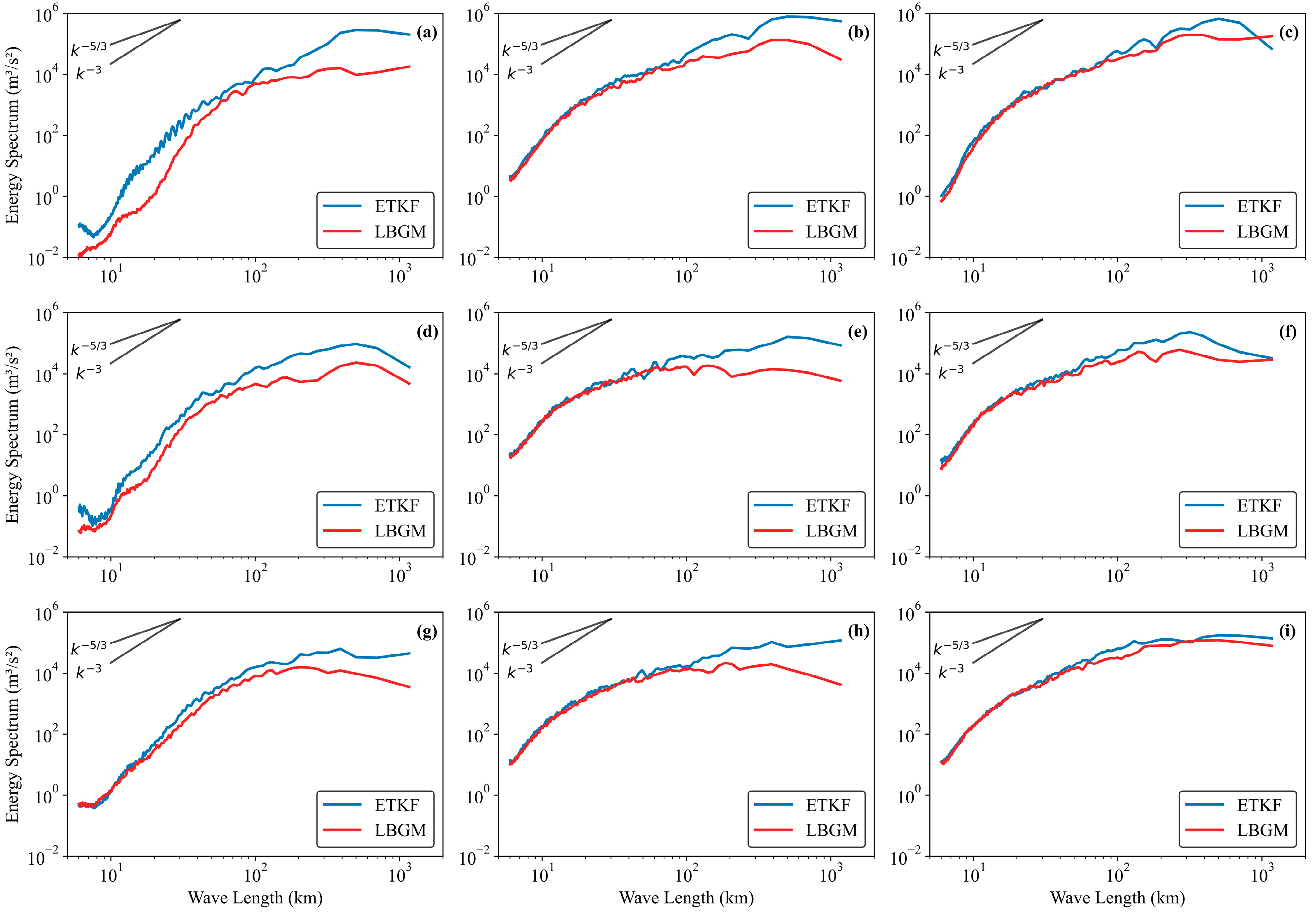
4.4. Kinetic Energy Spectrum Analysis
The kinetic energy spectrum reflects the energy distribution characteristics of initial perturbations across different scales and can be used to compare the reliability of model forecasts. This study applies the two-dimensional discrete cosine transform (2D-DCT) to perform spectral analysis on perturbation wind fields using different initial perturbation methods [
39]. The horizontal kinetic energy spectrum at each vertical level is calculated from horizontal perturbation wind fields (
).
Figure 8 shows the kinetic energy spectra at 200 hPa, 500 hPa, and 850 hPa levels for ETKF and LBGM methods across forecast lead times. Comparative analysis reveals that perturbation energy for both methods generally reaches maximum values at a 18-h forecast lead time across all wavelength ranges.
The overall characteristic of horizontal kinetic energy spectra at different vertical levels and forecast times is that spectral energy gradually increases with increasing wavelength. High-energy regions of the kinetic energy spectrum are mainly distributed in the 100–1000 km mesoscale range, likely associated with shortwave troughs and mesoscale shear line forcing. Within this range, the perturbation energy of the ETKF method is significantly higher than that of LBGM, indicating that ETKF captures more perturbation information above the meso- and meso- scales at all forecast lead times, potentially improving the description of weather systems such as low-level jets, low-level shear, and vortices.
For wavelengths within the small-scale range (below 100 km), the perturbation energy of both methods grows rapidly during the first 12 h forecast lead time and stabilizes afterward. At the initial time, the perturbation energy of ETKF within the 6–60 km scale range at 200 hPa and 500 hPa levels exceeds that of LBGM, suggesting that ETKF contains more small- to medium-scale perturbation information. In the mid-to-lower troposphere (500 hPa and 850 hPa), the spectral energy for wavelengths above 100 km increases with forecast lead time, while at upper levels (200 hPa), the growth becomes insignificant after 12 h, reflecting a gradual shift of perturbation energy adjustment toward the mid-to-lower troposphere.
Overall, ETKF exhibits an initial advantage over LBGM in small- to medium-scale perturbation energy. However, as forecast lead time increases, the small-scale energy of both methods stabilizes and becomes comparable, which is related to the limited development of small-scale perturbations due to nonlinear effects and dissipation [
40]. Meanwhile, ETKF significantly enhances the kinetic energy spectrum energy at scales above the meso-
and meso-
scales.
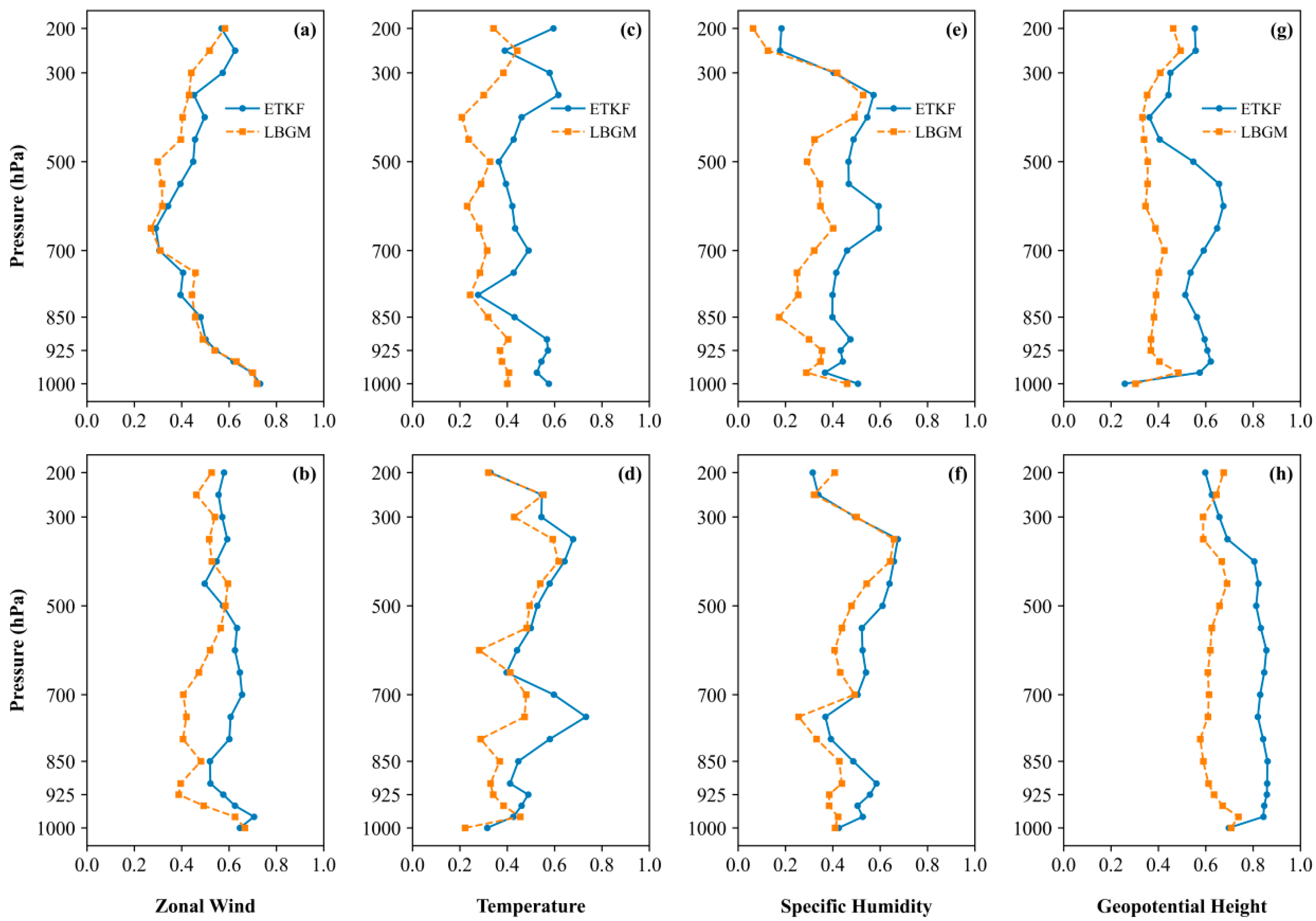
4.5. PECA Test
To further evaluate the effectiveness of perturbation structures in the two initial perturbation methods, the perturbation versus error correlation analysis (PECA) metric was calculated for model forecasts at different vertical levels and forecast lead times. The core of the PECA test lies in reducing the influence of model errors and analysis quality on perturbation quality assessment [
41], objectively quantifying the ability of ensemble perturbations to explain forecast errors. Higher PECA values indicate that ensemble perturbations effectively capture forecast errors, generating more valid perturbations.
Figure 9 shows the vertical distributions of PECA for the LBGM and ETKF methods at 12-h and 24-h forecast lead times. The ETKF method generally exhibits higher PECA values than LBGM, demonstrating its superior capability to capture forecast error information. The square of the PECA value represents the proportion of explained error variance. At the 12-hour lead time, the differences in PECA for zonal wind between ETKF and LBGM are small, mostly above 0.4, meaning that 16% of the error variance is explained by optimal perturbations. As the forecast lead time increases, PECA values for all variables increase across vertical levels, particularly for geopotential height, indicating that both initial perturbation methods effectively reflect the structural characteristics of geopotential height errors by the 24-h lead time. Approximately 36% (64%) of the error variance can be explained by the optimal perturbations of the LBGM (ETKF) method at different vertical levels.
4.6. Precipitation and Radar Echo Verification
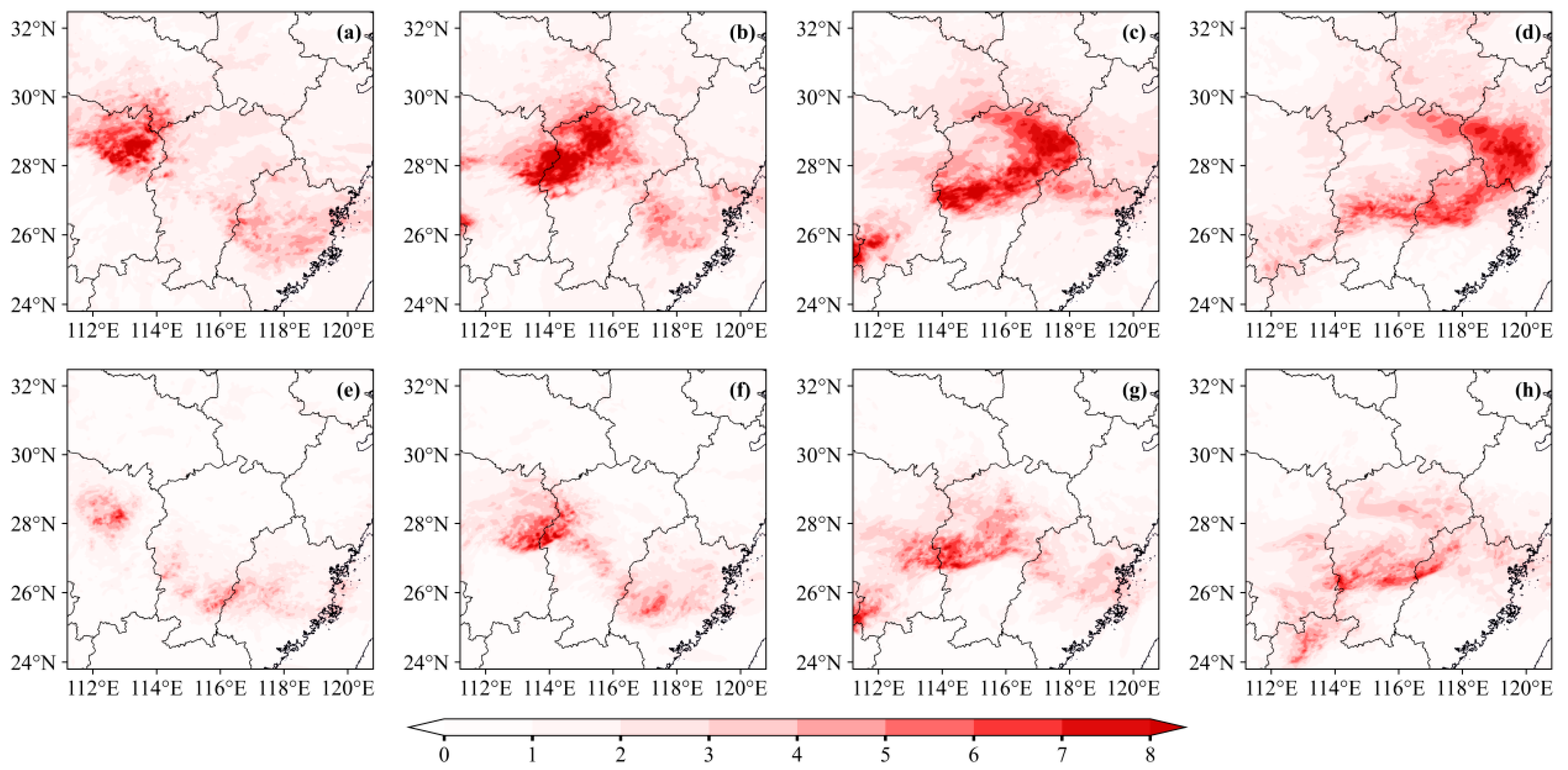
A reasonable initial perturbation structure is critical to ensuring the quality of ensemble forecast perturbations. To better understand the impacts of different perturbation structures from the two methods on ensemble forecasting performance, forecasts of heavy precipitation and the radar reflectivity factor during this squall line event were conducted and comparatively analyzed.
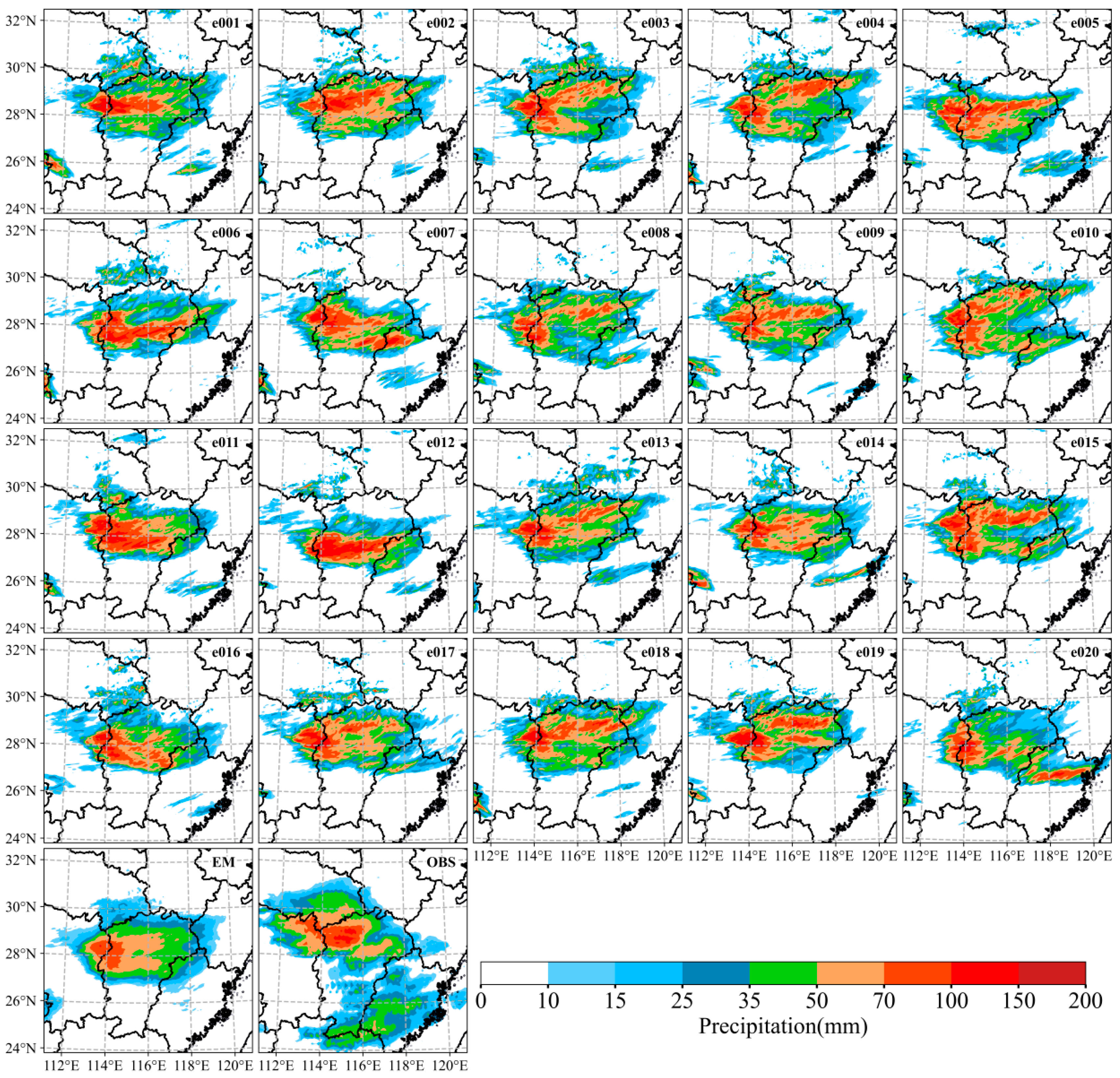
Figure 10 presents the accumulated precipitation observations from 1200 to 2000 UTC 30 March 2024 and the composite reflectivity observations at 1900 UTC 30 March during the squall line’s impact on Nanchang.
Figure 11 and
Figure 12 show the forecast accumulated precipitation distributions of the LBGM and ETKF methods, respectively, during the corresponding period in
Figure 10. Both methods successfully forecast the primary heavy precipitation distribution in northwestern Jiangxi Province. In
Figure 11, LBGM accurately reproduces the shape and orientation of the rainfall area; however, the main precipitation region exhibits a southward position bias. LBGM also forecasts rainfall areas in Fujian Province. Notably, the precipitation patterns among LBGM ensemble members show some consistency, which may be associated with their relatively low spread levels.
The precipitation distribution generated with the ETKF method is shifted northward compared to that of the LBGM method, exhibiting higher consistency with the observed precipitation within Jiangxi Province. However, the ETKF-generated precipitation areas are spatially more dispersed. As shown in
Figure 12, ensemble members (e.g., e001, e002, e018) successfully forecast the occurrence of heavy precipitation in Nanchang City, with their precipitation distributions positioned closer to observations. This robustly corroborates the earlier conclusion that the ETKF method is more likely to generate forecasts closer to observed weather systems.
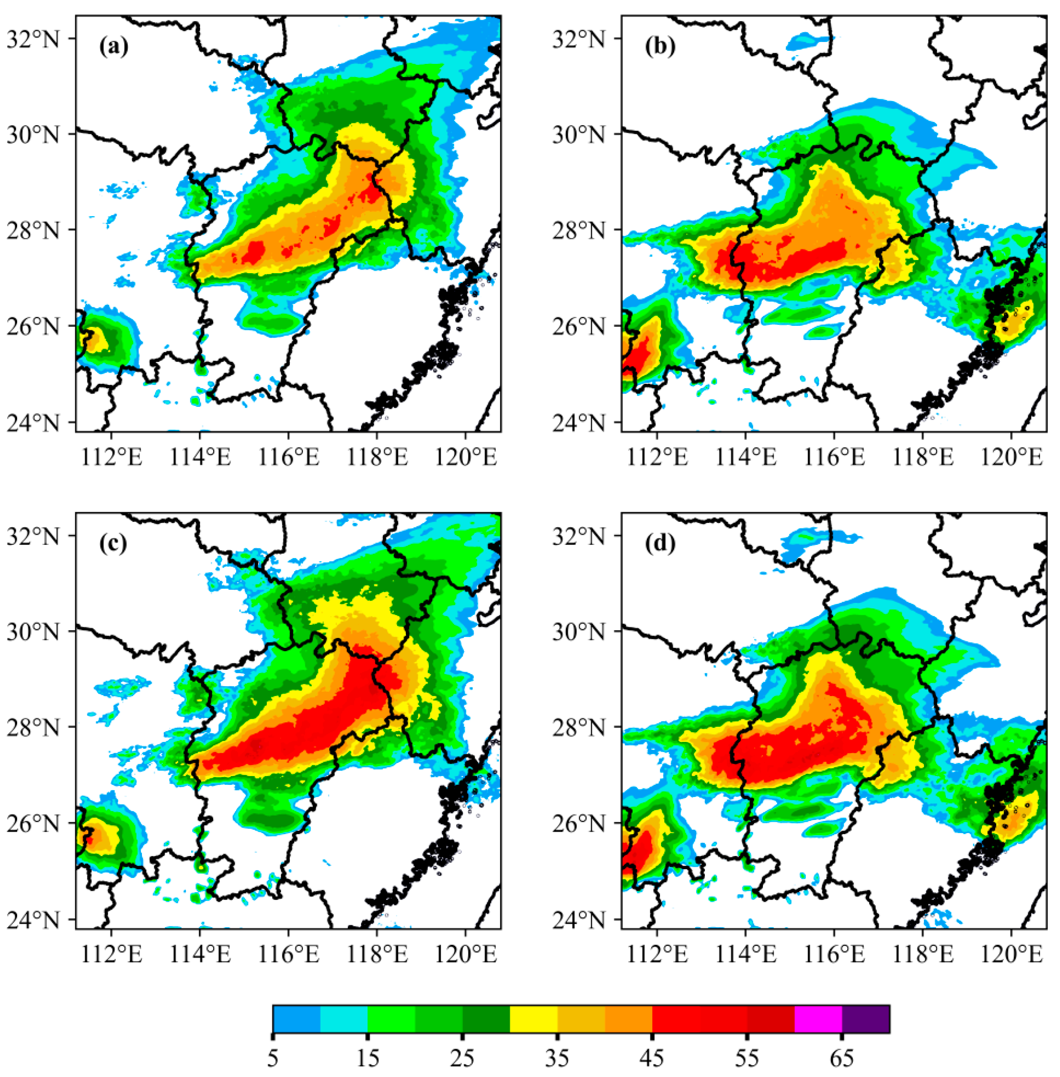
Figure 13 shows the ensemble mean and probability-matched mean-corrected radar reflectivity factor at the time corresponding to the observations in
Figure 10b. Both methods forecast echo positions largely consistent with the observed echo band. However, the ensemble mean, which integrates information from all members, smooths out high-reflectivity regions of individual members. The ensemble mean forecast of ETKF captures the bow-shaped structure of the squall line with reflectivity above 40 dBZ, albeit weaker than the observations. In contrast, the ensemble mean of LBGM forecasts a continuous bow-shaped strong echo above 45 dBZ, significantly improving echo intensity, but the >45 dBZ echo band shifts southeastward compared to observations.
The probability-matched mean-corrected radar reflectivity images (
Figure 13c,d) better reproduce the strong echo regions smoothed by simple ensemble averaging. Both methods successfully forecast the local echo protrusion at the right end of the strong echo band but exhibit notable differences. The ETKF method overextends the convective system axis north of 29.5° N, deviating from observations. Meanwhile, LBGM’s protrusion near Nanchang (28.2° N–28.8° N) aligns better with observed reflectivity but fails to capture echo development in northeastern Jiangxi (29.5° N–30.5° N). These spatial discrepancies likely contribute to systematic precipitation biases in northwestern Jiangxi.
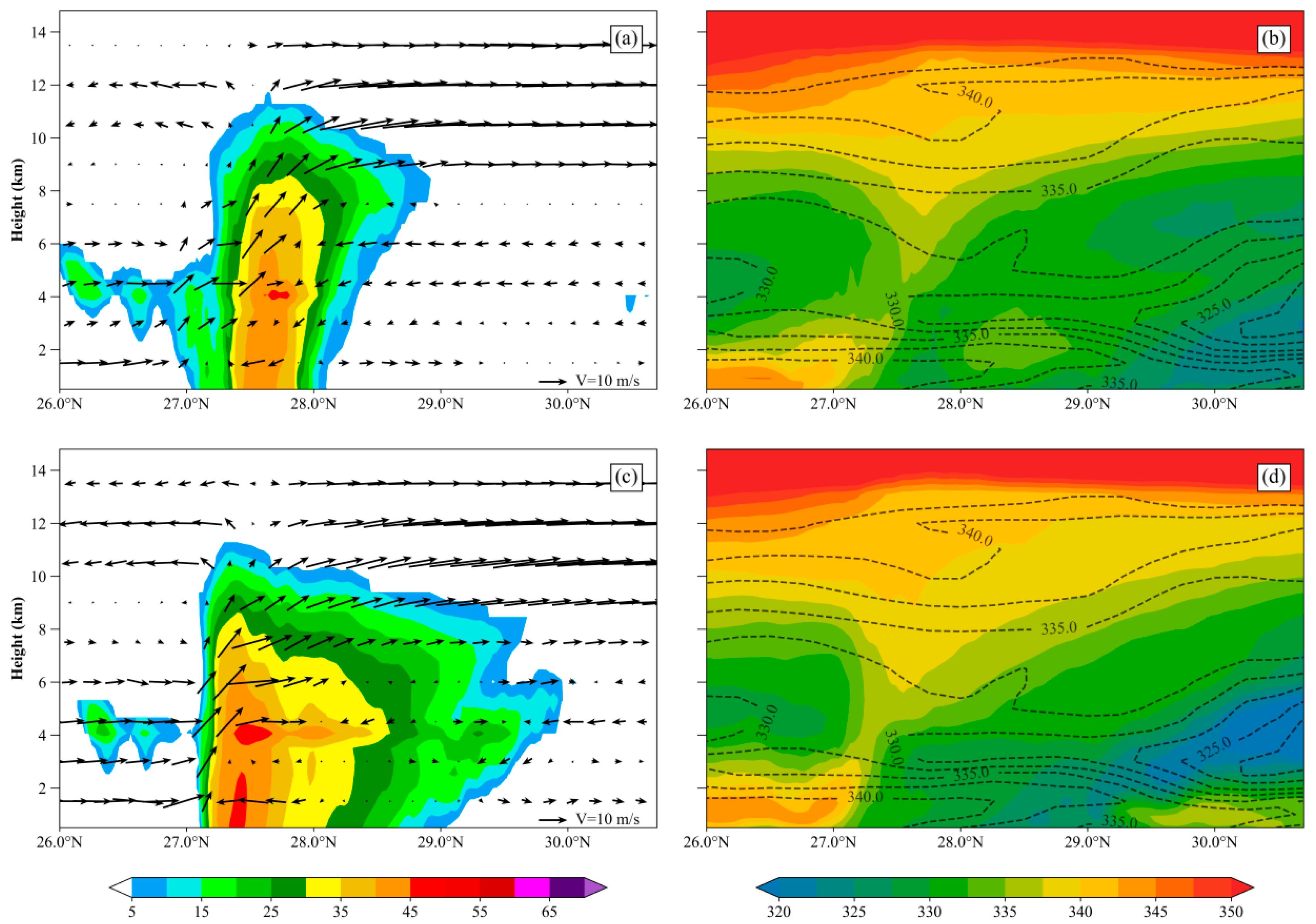
This study further compares the vertical cross-sectional structures of the squall line in the two ensemble forecast experiments.
Figure 14 constructs a meridional vertical cross-section along 115.3° E longitude (convective core region of the mature squall line over Nanchang) to compare the ensemble mean forecasts of radar reflectivity factor, wind fields, and pseudo-equivalent potential temperature between the two experiments. From the radar echo cross-sectional profiles, both ETKF and LBGM methods forecast vertically upright strong radar echo zones near 27.5° N. However, ETKF underestimates reflectivity intensity, with >45 dBZ echoes confined to 4 km altitude. In contrast, LBGM produces more continuous strong echo structures ahead of the squall line, with slightly higher echo tops, likely due to differences in vertical updraft speeds within the leading-edge low-level vertical wind shear (more pronounced in LBGM). The ETKF method more distinctly forecasts the vertical distribution of divergent sinking airflow near 28° N, but demonstrates biases in forecasting the vertical profile of pseudo-equivalent potential temperature. The LBGM method forecasts the position and altitude of the low pseudo-equivalent potential temperature region behind the squall line more closely aligned with observations. Through vertical advection of strong mid-level (4–5 km) subsidence, LBGM effectively transports dry, cold air to the surface, jointly facilitating cold pool formation—a critical mechanism sustaining squall line development.
5. Conclusions and Discussion
This study investigates the perturbation characteristics and forecast skill differences of two initial perturbation methods, namely, Local Breeding Growth Modes (LBGM) and Ensemble Transform Kalman Filter (ETKF), in ensemble forecasting of severe convective weather using an extreme squall line event in Nanchang, Jiangxi Province on 30–31 March 2024 as a case. The analysis incorporates metrics including root mean square error (RMSE) and ensemble spread consistency, evolution of total moist energy, kinetic energy spectrum distribution, perturbation versus error correlation analysis (PECA), precipitation, and radar reflectivity verification. The main conclusions are as follows.
The RMSE and ensemble spread consistency results show that LBGM significantly improves forecast accuracy for middle and upper troposphere variables and moderately enhances lower-tropospheric temperature fields. However, its ensemble spread is systematically lower than ETKF, leading to insufficient consistency between spread and forecast errors. Evaluated using PECA, ETKF outperforms LBGM in capturing forecast errors across all lead times.
The evolution of dynamical spread in both methods aligns with characteristics of severe convective systems, exhibiting flow-dependent features. ETKF perturbations develop rapidly with the squall line system, showing more physically realistic spread growth, particularly improving lower-tropospheric dynamical fields. In contrast, LBGM demonstrates superior spatial coherence of spread in the mid-upper troposphere but underperforms at lower levels.
The vertical distribution of total moist energy in both methods exhibits two peak regions: upper layers (300–100 hPa) dominated by jet stream-influenced kinetic energy and lower layers (1000–700 hPa) where kinetic energy and moist physics terms are equally significant. Initially, ETKF exhibits higher total moist energy than LBGM. Both methods show increasing total moist energy with forecast lead time, with ETKF exhibiting greater growth rates.
Kinetic energy spectrum analysis further reveals increasing perturbation spectral energy in both methods, concentrated in the 100–1000 km mesoscale range. Within this range, ETKF’s spectral energy markedly exceeds LBGM, indicating its enhanced capability to capture perturbations above meso- and meso- scales. At initial times, ETKF also demonstrates superior ability to resolve small- to medium-scale perturbations within the 6–60 km range.
Both methods demonstrate skill in forecasting squall line heavy precipitation, with ETKF better correcting systematic precipitation biases. Significant differences emerge in simulating the strong echo band east of the squall line. LBGM successfully reproduces the spatial structure of strong convective echoes around Nanchang but fails to capture precipitation echoes in northeastern Jiangxi. Meridional vertical cross-section analysis indicates that LBGM’s accurate depiction of leading-edge vertical updrafts and rear-sector low pseudo-equivalent potential temperature regions underpins its successful capture of localized intense echoes.


