
Assessment of PM10 and PM2.5 Concentrations in Santo Domingo: A Comparative Study Between 2019 and 2022
 , , , , ,
  and
and
Abstract
1. Introduction
2. Materials and Methods
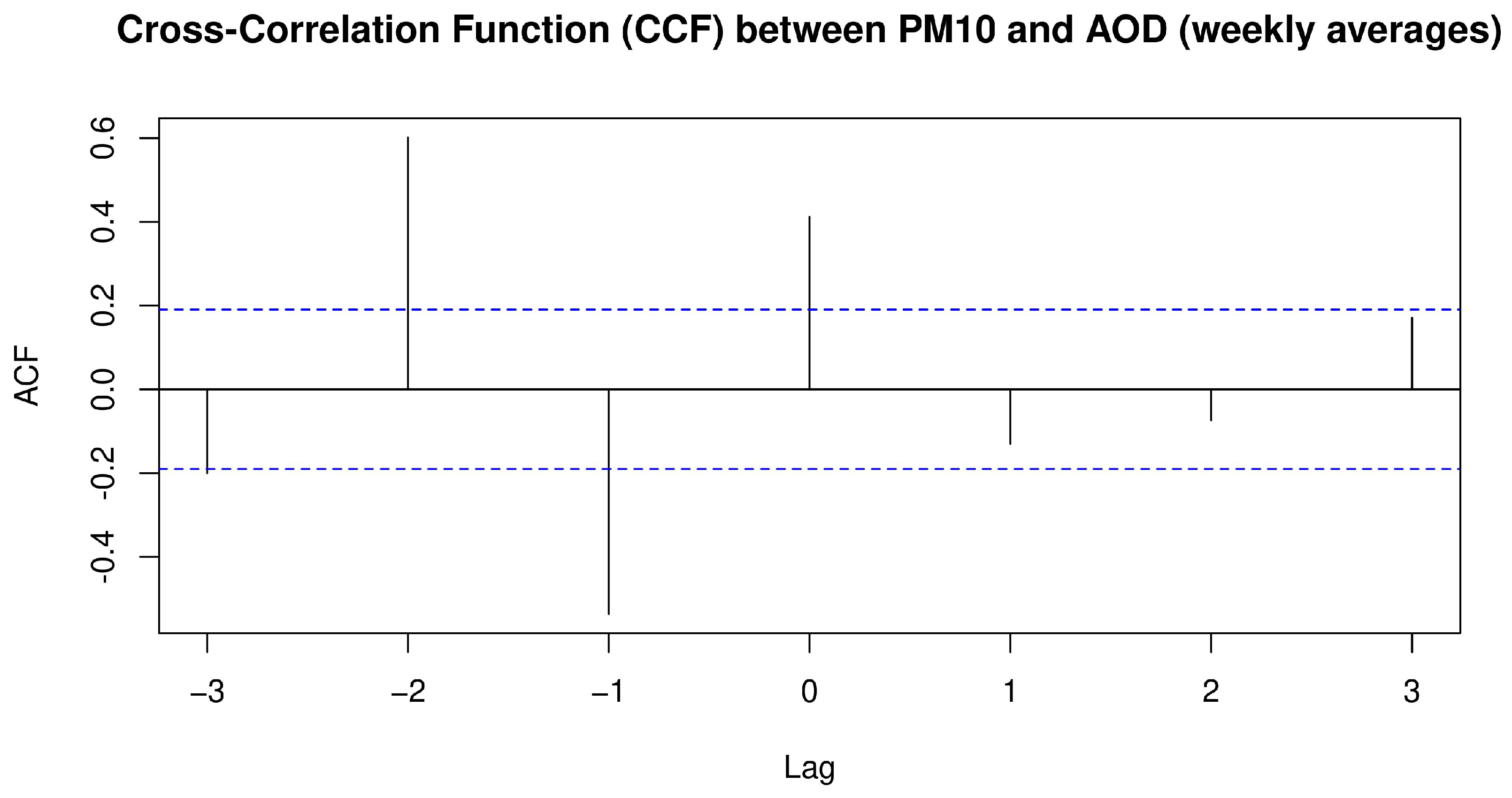
Data Analysis
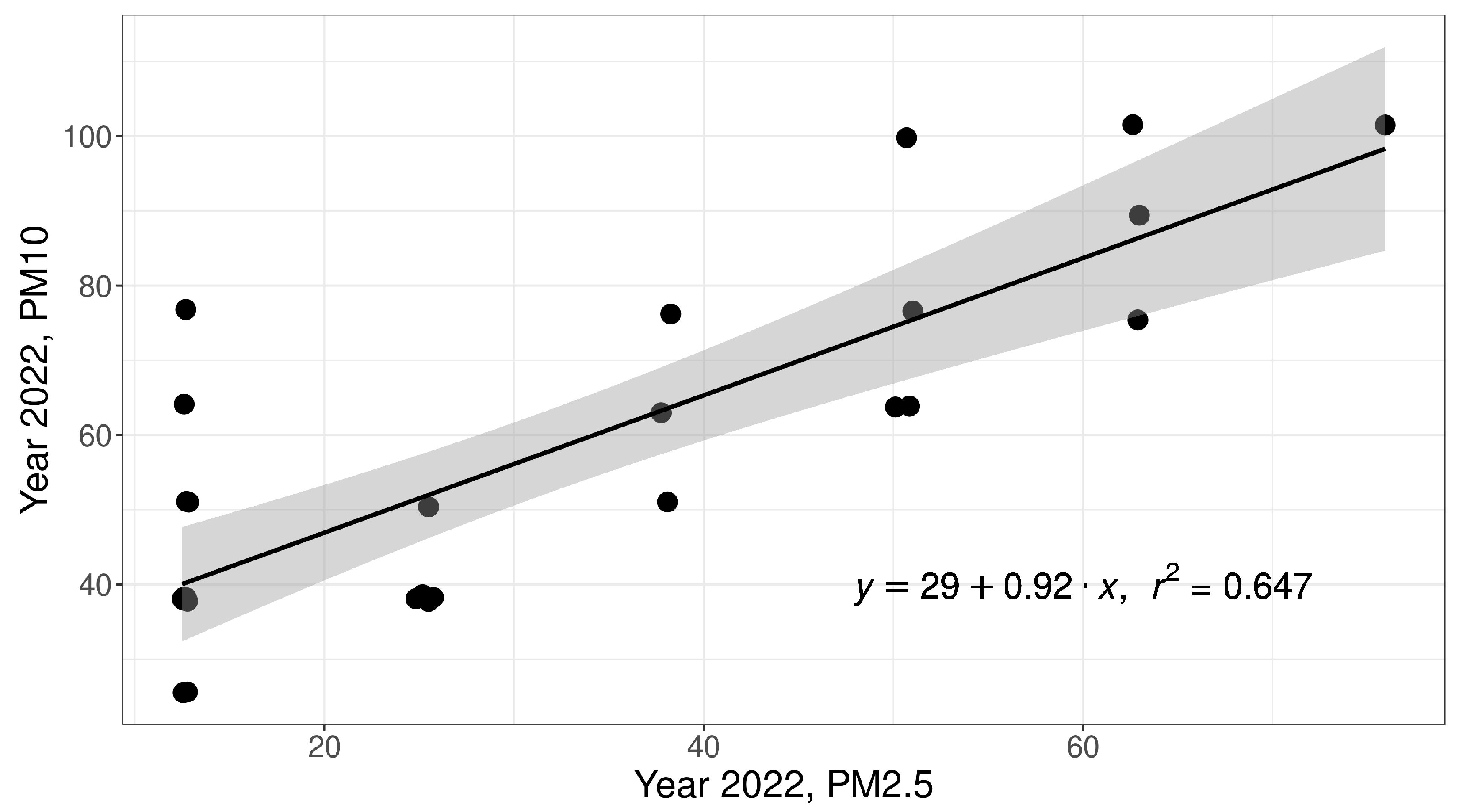
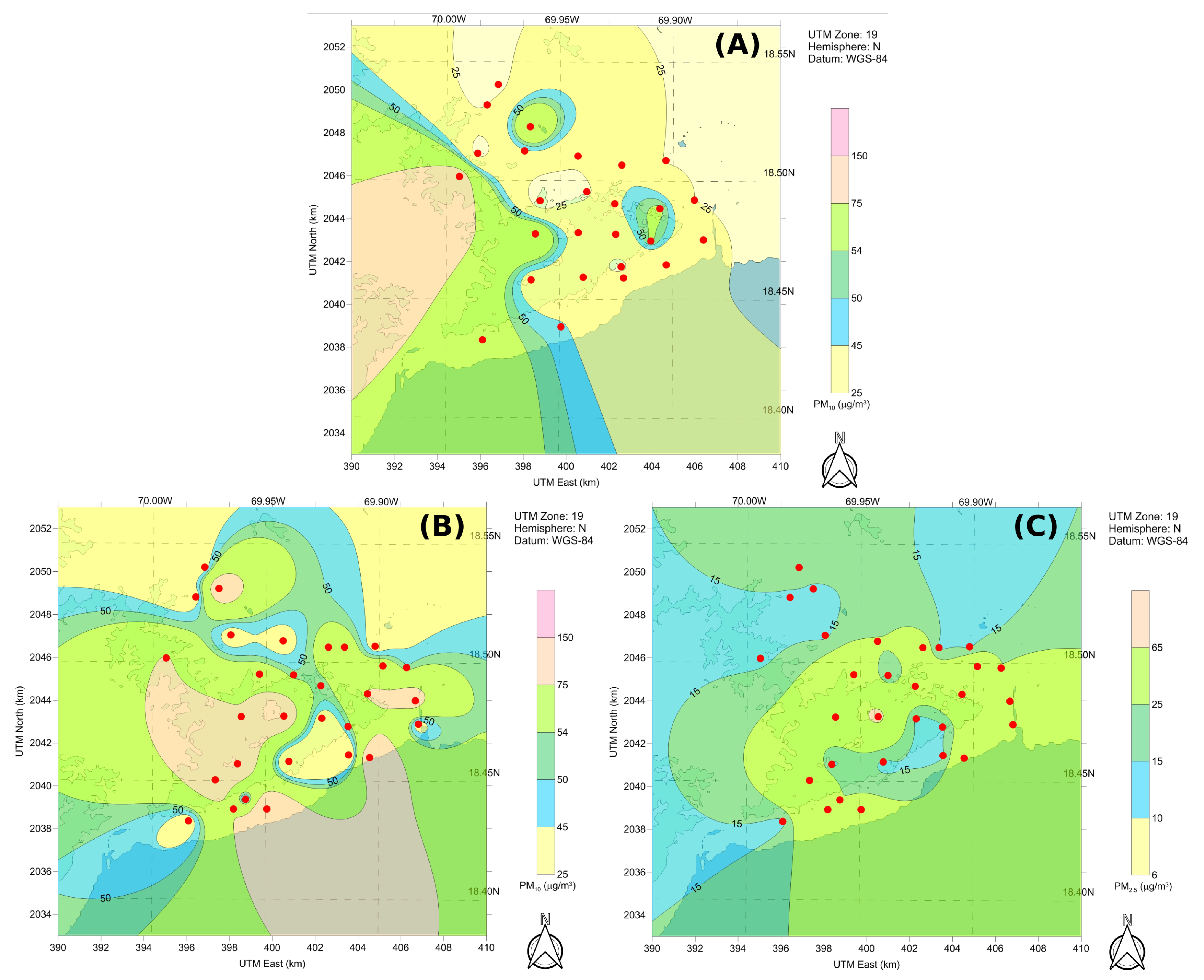
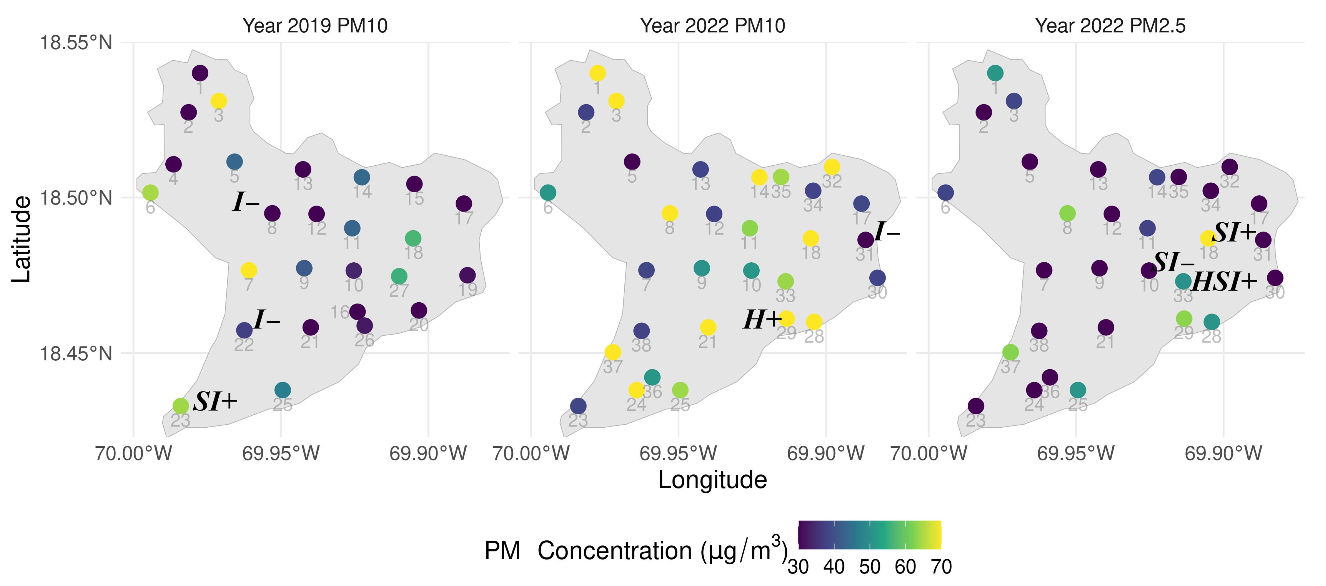
3. Results
4. Discussion
5. Conclusions
6. Recommendations
Author Contributions
Funding
Institutional Review Board Statement
Informed Consent Statement
Data Availability Statement
Acknowledgments
Conflicts of Interest
Abbreviations
| AOD | Aerosol Optical Depth |
| CCF | Cross-correlation functions |
| LISA | Local Indicators of Spatial Association |
| LOESS | Locally Estimated Scatterplot Smoothing |
| MAIAC | Multi-angle Implementation of Atmospheric Correction |
| PM | Particulate Matter |
| PM10 | Particles with a diameter less than 10 µm |
| PM2.5 | Particles with a diameter less than 2.5 µm |
Appendix A. Identifier Code (ID), English–Spanish Name Equivalence, Sampling Years (Marked with “x” for 2019 and/or 2022), and Geographic Coordinates of the Sampling Sites

| ID | Name in English | Name in Spanish | 2019 | 2022 | Latitude | Longitude |
|---|---|---|---|---|---|---|
| 1 | Prof. Adolfo González School | Liceo Prof. Adolfo González | x | x | 18.5400 | −69.9774 |
| 2 | Salomé Ureña de Henríquez (Los Girasoles) School | Escuela Básica Salomé Ureña de Henríquez (Los Girasoles) | x | x | 18.5274 | −69.9813 |
| 3 | Escuela Básica Prof. María del Carmen Pérez Méndez | Escuela Básica Prof. María del Carmen Pérez Méndez | x | x | 18.5310 | −69.9711 |
| 4 | Ciudad Real School | Colegio Ciudad Real | x | 18.5107 | −69.9864 | |
| 5 | The Community For Learning | The Community For Learning | x | x | 18.5115 | −69.9657 |
| 6 | José Bordas Valdez School | Escuela José Bordas Valdez | x | x | 18.5016 | −69.9942 |
| 7 | Los Prados School | Colegio Los Prados | x | x | 18.4766 | −69.9609 |
| 8 | National Botanical Garden | Jardín Botánico Nacional | x | x | 18.4949 | −69.9529 |
| 9 | Notre Dame School | Colegio Notre Dame | x | x | 18.4773 | −69.9421 |
| 10 | San Judas Tadeo School | Colegio San Judas Tadeo | x | x | 18.4765 | −69.9253 |
| 11 | Víctor Estrella Liz School | Instituto Politécnico Víctor Estrella Liz | x | x | 18.4901 | −69.9258 |
| 12 | Arroyo Hondo School | Colegio Arroyo Hondo | x | x | 18.4947 | −69.9379 |
| 13 | American School of Santo Domingo | American School of Santo Domingo | x | x | 18.5090 | −69.9425 |
| 14 | Padre Eulalio Antonio Arias Inoa School | Escuela Básica Padre Eulalio Antonio Arias Inoa-PAX | x | x | 18.5065 | −69.9226 |
| 15 | Salomé Ureña School | Escuela Básica Salomé Ureña (Capotillo) | x | 18.5043 | −69.9047 | |
| 16 | Santo Domingo School | Colegio Santo Domingo | x | 18.4633 | −69.9240 | |
| 17 | María Auxiliadora School | Escuela Primaria María Auxiliadora-Loma del Chivo | x | x | 18.4980 | −69.8880 |
| 18 | República Dominicana School | Escuela Primaria República Dominicana | x | x | 18.4869 | −69.9052 |
| 19 | República de Argentina School | Centro Educativo del Nivel Medio República de Argentina | x | 18.4750 | −69.8867 | |
| 20 | Babeque Inicial y Primaria School | Babeque Inicial y Primaria | x | 18.4637 | −69.9032 | |
| 21 | Padre Valentín Salinero School | Escuela Padre Valentín Salinero | x | x | 18.4582 | −69.9399 |
| 22 | Serafín de Asís School | Colegio Serafín de Asís | x | 18.4573 | −69.9624 | |
| 23 | Movearte Professional School | Movearte Escuela Técnico Profesional | x | x | 18.4330 | −69.9840 |
| 24 | Francisco Xavier Billini School | Escuela Primaria Francisco Xavier Billini | x | 18.4381 | −69.9642 | |
| 25 | Rosa Duarte School | Hogar Escuela Rosa Duarte | x | x | 18.4381 | −69.9494 |
| 26 | República de El Salvador Kindergarten | Jardín de Infancia República de El Salvador | x | 18.4588 | −69.9216 | |
| 27 | Iberoamericana University (UNIBE) | Universidad Iberoamericana (UNIBE) | x | 18.4747 | −69.9099 | |
| 28 | UASD Faculty Club | Club de Profesores de la UASD | x | 18.4600 | −69.9040 | |
| 29 | Faculty of Health Sciences, UASD | Antiguo Marión, Facultad de Ciencias de la Salud, UASD | x | 18.4610 | −69.9134 | |
| 30 | University Geographic Institute, UASD | Instituto Geográfico Universitario (IGU), UASD | x | 18.4742 | −69.8825 | |
| 31 | Association of Authorized Master Builders | Asociacion de Maestro Constructores de Obras Autorizados (AMACOA) | x | 18.4864 | −69.8866 | |
| 32 | Nuestra Señora del Carmen School | Politécnico Nuestra Señora del Carmen | x | 18.5098 | −69.8980 | |
| 33 | APEC University | Universidad APEC | x | 18.4730 | −69.9137 | |
| 34 | Capotillo School | Centro Educativo Capotillo | x | 18.5022 | −69.9044 | |
| 35 | Aida Cartagena Portalatín School | Escuela Básica Aida Cartagena Portalatín | x | 18.5066 | −69.9152 | |
| 36 | Governorship of Mirador Sur Park | Gobernación del Parque Mirador Sur (ADN) | x | 18.4422 | −69.9589 | |
| 37 | Agrarian Institute of Dominican Republic | Instituto Agrario Dominicano (IAD) | x | 18.4503 | −69.9722 | |
| 38 | Private residence | Vivienda particular | x | 18.4571 | −69.9625 |
References
- Anderson, J.O.; Thundiyil, J.G.; Stolbach, A. Clearing the Air: A Review of the Effects of Particulate Matter Air Pollution on Human Health. J. Med. Toxicol. 2012, 8, 166–175. [Google Scholar] [CrossRef] [PubMed]
- World Health Organization. The World Health Report 2002: Reducing Risks, Promoting Healthy Life; World Health Organization: Geneva, Switzerland, 2002.
- World Health Organization. WHO Global Air Quality Guidelines: Particulate Matter (PM2. 5 and PM10), Ozone, Nitrogen Dioxide, Sulfur Dioxide And Carbon Monoxide; World Health Organization: Geneva, Switzerland, 2021.
- Goossens, J.; Jonckheere, A.C.; Dupont, L.J.; Bullens, D.M.A. Air Pollution and the Airways: Lessons from a Century of Human Urbanization. Atmosphere 2021, 12, 898. [Google Scholar] [CrossRef]
- Anjum, M.S.; Ali, S.M.; Imad-ud-din, M.; Subhani, M.A.; Anwar, M.N.; Nizami, A.S.; Ashraf, U.; Khokhar, M.F. An Emerged Challenge of Air Pollution and Ever-Increasing Particulate Matter in Pakistan; A Critical Review. J. Hazard. Mater. 2021, 402, 123943. [Google Scholar] [CrossRef] [PubMed]
- Sicard, P.; Agathokleous, E.; Anenberg, S.C.; De Marco, A.; Paoletti, E.; Calatayud, V. Trends in urban air pollution over the last two decades: A global perspective. Sci. Total Environ. 2023, 858, 160064. [Google Scholar] [CrossRef]
- Sanda, M.; Dunea, D.; Iordache, S.; Predescu, L.; Predescu, M.; Pohoata, A.; Onutu, I. Recent Urban Issues Related to Particulate Matter in Ploiesti City, Romania. Atmosphere 2023, 14, 746. [Google Scholar] [CrossRef]
- Wang, Z.; Chen, J.; Zhou, C.; Wang, S.; Li, M. The Impacts of Urban Form on PM2.5 Concentrations: A Regional Analysis of Cities in China from 2000 to 2015. Atmosphere 2022, 13, 963. [Google Scholar] [CrossRef]
- Xiao, K.; Wang, Y.; Wu, G.; Fu, B.; Zhu, Y. Spatiotemporal Characteristics of Air Pollutants (PM10, PM2.5, SO2, NO2, O3, and CO) in the Inland Basin City of Chengdu, Southwest China. Atmosphere 2018, 9, 74. [Google Scholar] [CrossRef]
- Asif, M.; Yousuf, S.; Donald, A.N.; Hassan, A.M.M.; Iqbal, A.; Bodlah, M.A.; Sharf, B.; Noshia, N. A review on particulate matter and heavy metal emissions; impacts on the environment, detection techniques and control strategies. Moj Ecol. Environ. Sci. 2021, 7, 1–5. [Google Scholar] [CrossRef]
- Karthick Raja Namasivayam, S.; Priyanka, S.; Lavanya, M.; Krithika Shree, S.; Francis, A.; Avinash, G.; Arvind Bharani, R.; Kavisri, M.; Moovendhan, M. A review on vulnerable atmospheric aerosol nanoparticles: Sources, impact on the health, ecosystem and management strategies. J. Environ. Manag. 2024, 365, 121644. [Google Scholar] [CrossRef]
- Fameli, K.M.; Moustris, K.; Spyropoulos, G.; Rodanas, D.M. Exposure to PM2.5 on Public Transport: Guidance for Field Measurements with Low-Cost Sensors. Atmosphere 2024, 15, 330. [Google Scholar] [CrossRef]
- Bessagnet, B.; Allemand, N.; Putaud, J.P.; Couvidat, F.; André, J.M.; Simpson, D.; Pisoni, E.; Murphy, B.N.; Thunis, P. Emissions of Carbonaceous Particulate Matter and Ultrafine Particles from Vehicles—A Scientific Review in a Cross-Cutting Context of Air Pollution and Climate Change. Appl. Sci. 2022, 12, 3623. [Google Scholar] [CrossRef] [PubMed]
- Contini, D.; Cesari, D.; Donateo, A.; Chirizzi, D.; Belosi, F. Characterization of PM10 and PM2.5 and Their Metals Content in Different Typologies of Sites in South-Eastern Italy. Atmosphere 2014, 5, 435–453. [Google Scholar] [CrossRef]
- Alwadei, M.; Srivastava, D.; Alam, M.S.; Shi, Z.; Bloss, W.J. Chemical characteristics and source apportionment of particulate matter (PM2.5) in Dammam, Saudi Arabia: Impact of dust storms. Atmos. Environ. X 2022, 14, 100164. [Google Scholar] [CrossRef]
- Manousakas, M.I. Special Issue Sources and Composition of Ambient Particulate Matter. Atmosphere 2021, 12, 462. [Google Scholar] [CrossRef]
- Plocoste, T.; Laventure, S. Forecasting PM10 Concentrations in the Caribbean Area Using Machine Learning Models. Atmosphere 2023, 14, 134. [Google Scholar] [CrossRef]
- Sadiq, A.A. Effect of Particulate Emissions from Road Transportation Vehicles on Health of Communities in Urban and Rural Areas, Kano State, Nigeria. Ph.D. Thesis, Université Claude Bernard-Lyon I, Villeurbanne, France, 2022. [Google Scholar]
- Sawyer, W.E.; Aigberua, A.O.; Nwodo, M.U.; Akram, M. Overview of Air Pollutants and Their One Health Effects. In Air Pollutants in the Context of One Health: Fundamentals, Sources, and Impacts; Springer Nature: Cham, Switzerland, 2024; pp. 3–30. [Google Scholar] [CrossRef]
- Bae, M.; Kim, B.U.; Kim, H.C.; Kim, S. A Multiscale Tiered Approach to Quantify Contributions: A Case Study of PM2.5 in South Korea During 2010–2017. Atmosphere 2020, 11, 141. [Google Scholar] [CrossRef]
- Sacks, J.D.; Fann, N.; Gumy, S.; Kim, I.; Ruggeri, G.; Mudu, P. Quantifying the Public Health Benefits of Reducing Air Pollution: Critically Assessing the Features and Capabilities of WHO’s AirQ+ and U.S. EPA’s Environmental Benefits Mapping and Analysis Program—Community Edition (BenMAP—CE). Atmosphere 2020, 11, 516. [Google Scholar] [CrossRef]
- Xing, Y.F.; Xu, Y.H.; Shi, M.H.; Lian, Y.X. The impact of PM2.5 on the human respiratory system. J. Thorac. Dis. 2016, 8, E69–E74. [Google Scholar] [CrossRef]
- Thangavel, P.; Park, D.; Lee, Y.C. Recent Insights into Particulate Matter (PM2.5)-Mediated Toxicity in Humans: An Overview. Int. J. Environ. Res. Public Health 2022, 19, 7511. [Google Scholar] [CrossRef]
- Alharbi, H.A.; Rushdi, A.I.; Bazeyad, A.; Al-Mutlaq, K.F. Temporal Variations, Air Quality, Heavy Metal Concentrations, and Environmental and Health Impacts of Atmospheric PM2.5 and PM10 in Riyadh City, Saudi Arabia. Atmosphere 2024, 15, 1448. [Google Scholar] [CrossRef]
- Billet, S.; Landkocz, Y.; Martin, P.J.; Verdin, A.; Ledoux, F.; Lepers, C.; André, V.; Cazier, F.; Sichel, F.; Shirali, P.; et al. Chemical characterization of fine and ultrafine PM, direct and indirect genotoxicity of PM and their organic extracts on pulmonary cells. J. Environ. Sci. 2018, 71, 168–178. [Google Scholar] [CrossRef] [PubMed]
- Velali, E.; Papachristou, E.; Pantazaki, A.; Choli-Papadopoulou, T.; Argyrou, N.; Tsourouktsoglou, T.; Lialiaris, S.; Constantinidis, A.; Lykidis, D.; Lialiaris, T.S.; et al. Cytotoxicity and genotoxicity induced in vitro by solvent-extractable organic matter of size-segregated urban particulate matter. Environ. Pollut. 2016, 218, 1350–1362. [Google Scholar] [CrossRef] [PubMed]
- Zou, Y.; Wu, Y.; Wang, Y.; Li, Y.; Jin, C. Physicochemical properties, in vitro cytotoxic and genotoxic effects of PM1.0 and PM2.5 from Shanghai, China. Environ. Sci. Pollut. Res. 2017, 24, 19508–19516. [Google Scholar] [CrossRef] [PubMed]
- Wang, M.; Kim, R.Y.; Kohonen-Corish, M.R.J.; Chen, H.; Donovan, C.; Oliver, B.G. Particulate matter air pollution as a cause of lung cancer: Epidemiological and experimental evidence. Br. J. Cancer 2025. [Google Scholar] [CrossRef]
- Veerappan, I.; Sankareswaran, S.K.; Palanisamy, R. Morin Protects Human Respiratory Cells from PM2.5 Induced Genotoxicity by Mitigating ROS and Reverting Altered miRNA Expression. Int. J. Environ. Res. Public Health 2019, 16, 2389. [Google Scholar] [CrossRef]
- Goudarzi, G.; Shirmardi, M.; Naimabadi, A.; Ghadiri, A.; Sajedifar, J. Chemical and organic characteristics of PM2.5 particles and their in-vitro cytotoxic effects on lung cells: The Middle East dust storms in Ahvaz, Iran. Sci. Total Environ. 2019, 655, 434–445. [Google Scholar] [CrossRef]
- Galeano-Páez, C.; Brango, H.; Pastor-Sierra, K.; Coneo-Pretelt, A.; Arteaga-Arroyo, G.; Peñata-Taborda, A.; Espitia-Pérez, P.; Ricardo-Caldera, D.; Humanez-Álvarez, A.; Londoño-Velasco, E.; et al. Genotoxicity and Cytotoxicity Induced In Vitro by Airborne Particulate Matter (PM2.5) from an Open-Cast Coal Mining Area. Atmosphere 2024, 15, 1420. [Google Scholar] [CrossRef]
- Chen, W.; Ge, P.; Deng, M.; Liu, X.; Lu, Z.; Yan, Z.; Chen, M.; Wang, J. Toxicological responses of A549 and HCE-T cells exposed to fine particulate matter at the air–liquid interface. Environ. Sci. Pollut. Res. 2024, 31, 27375–27387. [Google Scholar] [CrossRef]
- Figueiredo, D.; Vicente, E.D.; Vicente, A.; Gonçalves, C.; Lopes, I.; Alves, C.A.; Oliveira, H. Toxicological and Mutagenic Effects of Particulate Matter from Domestic Activities. Toxics 2023, 11, 505. [Google Scholar] [CrossRef]
- Hu, A.; Li, R.; Chen, G.; Chen, S. Impact of Respiratory Dust on Health: A Comparison Based on the Toxicity of PM2.5, Silica, and Nanosilica. Int. J. Mol. Sci. 2024, 25, 7654. [Google Scholar] [CrossRef]
- Tran, H.M.; Tsai, F.J.; Lee, Y.L.; Chang, J.H.; Chang, L.T.; Chang, T.Y.; Chung, K.F.; Kuo, H.P.; Lee, K.Y.; Chuang, K.J.; et al. The impact of air pollution on respiratory diseases in an era of climate change: A review of the current evidence. Sci. Total Environ. 2023, 898, 166340. [Google Scholar] [CrossRef] [PubMed]
- Orellano, P.; Reynoso, J.; Quaranta, N.; Bardach, A.; Ciapponi, A. Short-term exposure to particulate matter (PM10 and PM2.5), nitrogen dioxide (NO2), and ozone (O3) and all-cause and cause-specific mortality: Systematic review and meta-analysis. Environ. Int. 2020, 142, 105876. [Google Scholar] [CrossRef] [PubMed]
- Guo, C.; Lv, S.; Liu, Y.; Li, Y. Biomarkers for the adverse effects on respiratory system health associated with atmospheric particulate matter exposure. J. Hazard. Mater. 2022, 421, 126760. [Google Scholar] [CrossRef]
- Krittanawong, C.; Qadeer, Y.K.; Hayes, R.B.; Wang, Z.; Thurston, G.D.; Virani, S.; Lavie, C.J. PM2.5 and cardiovascular diseases: State-of-the-Art review. Int. J. Cardiol. Cardiovasc. Risk Prev. 2023, 19, 200217. [Google Scholar] [CrossRef]
- Anjum, S.; Zafar, M.M.; Kumari, A. Chapter 6—A review of diseases attributed to air pollution and associated health issues: A case study of Indian metropolitan cities. In Diseases and Health Consequences of Air Pollution; Dehghani, M.H., Karri, R.R., Vera, T., Hassan, S.K.M., Eds.; Academic Press: Cambridge, MA, USA, 2024; pp. 145–169. [Google Scholar] [CrossRef]
- Wan Mahiyuddin, W.R.; Ismail, R.; Mohammad Sham, N.; Ahmad, N.I.; Nik Hassan, N.M.N. Cardiovascular and Respiratory Health Effects of Fine Particulate Matters (PM2.5): A Review on Time Series Studies. Atmosphere 2023, 14, 856. [Google Scholar] [CrossRef]
- Li, Q.Q.; Guo, Y.T.; Yang, J.Y.; Liang, C.S. Review on main sources and impacts of urban ultrafine particles: Traffic emissions, nucleation, and climate modulation. Atmos. Environ. X 2023, 19, 100221. [Google Scholar] [CrossRef]
- Rahman, M.; Meng, L. Examining the Spatial and Temporal Variation of PM2.5 and Its Linkage with Meteorological Conditions in Dhaka, Bangladesh. Atmosphere 2024, 15, 1426. [Google Scholar] [CrossRef]
- Rusca, M.; Rusu, T.; Avram, S.E.; Prodan, D.; Paltinean, G.A.; Filip, M.R.; Ciotlaus, I.; Pascuta, P.; Rusu, T.A.; Petean, I. Physicochemical Assessment of the Road Vehicle Traffic Pollution Impact on the Urban Environment. Atmosphere 2023, 14, 862. [Google Scholar] [CrossRef]
- Dyer, G.M.; Khomenko, S.; Adlakha, D.; Anenberg, S.; Behnisch, M.; Boeing, G.; Esperon-Rodriguez, M.; Gasparrini, A.; Khreis, H.; Kondo, M.C.; et al. Exploring the nexus of urban form, transport, environment and health in large-scale urban studies: A state-of-the-art scoping review. Environ. Res. 2024, 257, 119324. [Google Scholar] [CrossRef]
- Wu, C.; Lu, S.; Tian, J.; Yin, L.; Wang, L.; Zheng, W. Current Situation and Prospect of Geospatial AI in Air Pollution Prediction. Atmosphere 2024, 15, 1411. [Google Scholar] [CrossRef]
- Jurado, X.; Reiminger, N.; Maurer, L.; Vazquez, J.; Wemmert, C. On the Correlations between Particulate Matter: Comparison between Annual/Monthly Concentrations and PM10/PM2.5. Atmosphere 2023, 14, 385. [Google Scholar] [CrossRef]
- Lightstone, S.; Gross, B.; Moshary, F.; Castillo, P. Development and Assessment of Spatially Continuous Predictive Algorithms for Fine Particulate Matter in New York State. Atmosphere 2021, 12, 315. [Google Scholar] [CrossRef]
- Zhao, C.; Pan, Y.; Teng, Y.; Baqa, M.F.; Guo, W. Air Quality Improvement in China: Evidence from PM2.5 Concentrations in Five Urban Agglomerations, 2000–2021. Atmosphere 2022, 13, 1839. [Google Scholar] [CrossRef]
- Shoari, N.; Dubé, J.S. Toward improved analysis of concentration data: Embracing nondetects. Environ. Toxicol. Chem. 2018, 37, 643–656. [Google Scholar] [CrossRef]
- Beloconi, A.; Chrysoulakis, N.; Lyapustin, A.; Utzinger, J.; Vounatsou, P. Bayesian geostatistical modelling of PM10 and PM2.5 surface level concentrations in Europe using high-resolution satellite-derived products. Environ. Int. 2018, 121, 57–70. [Google Scholar] [CrossRef]
- Adly, H.M.; Saleh, S.A.K. Long-Term Trends in PM10, PM2.5, and Trace Elements in Ambient Air: Environmental and Health Risks from 2020 to 2024. Atmosphere 2025, 16, 415. [Google Scholar] [CrossRef]
- Wang, W.; Zhang, G.; Luo, Y.; Liang, X.; Liu, L.; Luo, K.; Xiao, Y. The Correlation Between Surface Temperature and Surface PM2.5 in Nanchang Region, China. Atmosphere 2025, 16, 411. [Google Scholar] [CrossRef]
- Giarra, A.; Riccio, A.; Chianese, E.; Annetta, M.; Toscanesi, M.; Trifuoggi, M. Transport Mechanisms and Pollutant Dynamics Influencing PM10 Levels in a Densely Urbanized and Industrialized Region near Naples, South Italy: A Residence Time Analysis. Atmosphere 2025, 16, 393. [Google Scholar] [CrossRef]
- Haj Ismail, A.; Dawi, E.A.; Almokdad, N.; Abdelkader, A.; Salem, O. Estimation and Comparison of the Clearness Index using Mathematical Models—Case study in the United Arab Emirates. Evergreen 2023, 10, 863–869. [Google Scholar] [CrossRef]
- Haj Ismail, A.A.K. Prediction of Global Solar Radiation from Sunrise Duration Using Regression Functions. Kuwait J. Sci. 2021, 49, 15051. [Google Scholar] [CrossRef]
- Morphet, W.J. Simulation, Kriging, and Visualization of Circular-Spatial Data. Ph.D. Thesis, Utah State University, Old Main Hill Logan, UT, USA, 2009. [Google Scholar] [CrossRef]
- Wu, S.; Huang, B.; Wang, J.; He, L.; Wang, Z.; Yan, Z.; Lao, X.; Zhang, F.; Liu, R.; Du, Z. Spatiotemporal mapping and assessment of daily ground NO2 concentrations in China using high-resolution TROPOMI retrievals. Environ. Pollut. 2021, 273, 116456. [Google Scholar] [CrossRef] [PubMed]
- Zhang, H.; Li, N.; Tang, K.; Liao, H.; Shi, C.; Huang, C.; Wang, H.; Guo, S.; Hu, M.; Ge, X.; et al. Estimation of secondary PM2.5 in China and the United States using a multi-tracer approach. Atmos. Chem. Phys. 2022, 22, 5495–5514. [Google Scholar] [CrossRef]
- Tang, B.; Stanier, C.O.; Carmichael, G.R.; Gao, M. Ozone, nitrogen dioxide, and PM2.5 estimation from observation-model machine learning fusion over S. Korea: Influence of observation density, chemical transport model resolution, and geostationary remotely sensed AOD. Atmos. Environ. 2024, 331, 120603. [Google Scholar] [CrossRef]
- Ahmed, A.; Bin Ali, A.A.; Mahboob, M.; Humaira, F. Comparison between Local and Global Methods to Develop AQI in Representing the Spatial Pattern of Air Quality of Dhaka City. Dhaka Univ. J. Earth Environ. Sci. 2023, 11, 131–149. [Google Scholar] [CrossRef]
- Hernández-Ceballos, M.; López-Orozco, R.; Ruiz, P.; Galán, C.; García-Mozo, H. Exploring the influence of meteorological conditions on the variability of olive pollen intradiurnal patterns: Differences between pre- and post-peak periods. Sci. Total Environ. 2024, 956, 177231. [Google Scholar] [CrossRef]
- Espinal, G.; Nivar, S. Estudio de la contaminación ambiental al interior de las viviendas en tres barrios de la capital dominicana. Cienc. Soc. 2004, 29, 167–212. [Google Scholar] [CrossRef]
- Caballero-González, C. Calidad del Aire e Infraestructura Verde. Estudio de caso: Distrito Nacional. Master’s Thesis, Instituto Tecnológico de Santo Domingo (INTEC), Santo Domingo, Dominican Republic, 2020. [Google Scholar]
- Gómez Pérez, A.; Guillermo Manzanillo, L.A.; Vázquez Frías, J.; Quintana Pérez, C.E. Contaminación atmosférica en puntos seleccionados de la ciudad de Santo Domingo, República Dominicana. Cienc. Soc. 2014, 39, 533–557. [Google Scholar] [CrossRef]
- Vallejo Díaz, A.; Herrera Moya, I. Urban wind energy with resilience approach for sustainable cities in tropical regions: A review. Renew. Sustain. Energy Rev. 2024, 199, 114525. [Google Scholar] [CrossRef]
- Fernández, I.C.; Koplow-Villavicencio, T.; Montoya-Tangarife, C. Urban environmental inequalities in Latin America: A scoping review. World Dev. Sustain. 2023, 2, 100055. [Google Scholar] [CrossRef]
- Martinuzzi, S.; Locke, D.H.; Ramos-González, O.; Sanchez, M.; Grove, J.M.; Muñoz-Erickson, T.A.; Arendt, W.J.; Bauer, G. Exploring the relationships between tree canopy cover and socioeconomic characteristics in tropical urban systems: The case of Santo Domingo, Dominican Republic. Urban For. Urban Green. 2021, 62, 127125. [Google Scholar] [CrossRef]
- Bonilla-Duarte, S.; González, C.C.; Rodríguez, L.C.; Jáuregui-Haza, U.J.; García-García, A. Contribution of Urban Forests to the Ecosystem Service of Air Quality in the City of Santo Domingo, Dominican Republic. Forests 2021, 12, 1249. [Google Scholar] [CrossRef]
- Hernández-Garces, A.; Peña-Cossío, R.; Hernández Bilbao, F.; González, J.A. Distribución espacial de la emisión de contaminantes a la atmósfera emitidos por centrales azucareros villaclareños. Cent. Azú Car 2021, 48, 29–40. [Google Scholar]
- Liu, H.Y.; Schneider, P.; Haugen, R.; Vogt, M. Performance Assessment of a Low-Cost PM2.5 Sensor for a near Four-Month Period in Oslo, Norway. Atmosphere 2019, 10, 41. [Google Scholar] [CrossRef]
- Airmetrics. MiniVol Portable Air Sampler Operation Manual; Airmetrics: Eugene, OR, USA, 2007. [Google Scholar]
- Airmetrics. MiniVol TAS Portable Air Sampler; Airmetrics: Eugene, OR, USA, 2024. [Google Scholar]
- Triola, M. Estadística (Décima Edición); Pearson Educación: Ciudad de México, Mexico, 2009. [Google Scholar]
- Becker, R.; Chambers, J.; Wilks, A. The New S Language: A Programming Environment for Data Analysis and Graphics; Computer Science Serxies; Wadsworth & Brooks/Cole Advanced Books & Software; Springer: Berlin/Heidelberg, Germany, 1988. [Google Scholar]
- Venables, W.N.; Ripley, B.D.; Venables, W.N. Modern Applied Statistics with S, 4th ed.; Statistics and Computing; Springer: New York, NY, USA, 2002; OCLC: ocm49312402. [Google Scholar]
- Zeileis, A.; Grothendieck, G. zoo: S3 Infrastructure for Regular and Irregular Time Series. J. Stat. Softw. 2005, 14, 1–27. [Google Scholar] [CrossRef]
- Hyndman, R.J.; Khandakar, Y. Automatic time series forecasting: The forecast package for R. J. Stat. Softw. 2008, 27, 1–22. [Google Scholar] [CrossRef]
- Hyndman, R.; Athanasopoulos, G.; Bergmeir, C.; Caceres, G.; Chhay, L.; O’Hara-Wild, M.; Petropoulos, F.; Razbash, S.; Wang, E.; Yasmeen, F. Forecast: Forecasting Functions for Time Series and Linear Models; R Package Version 8.22.0; CRAN: Windhoek, Namibia, 2024. [Google Scholar]
- Hyndman, R.J.; Killick, R. CRAN Task View: Time Series Analysis; Comprehensive R Archive Network (CRAN): Windhoek, Namibia, 2024. [Google Scholar]
- Abdullah, S.; Ismail, M.; Ahmed, A.N.; Abdullah, A.M. Forecasting Particulate Matter Concentration Using Linear and Non-Linear Approaches for Air Quality Decision Support. Atmosphere 2019, 10, 667. [Google Scholar] [CrossRef]
- Moran, P.A. The interpretation of statistical maps. J. R. Stat. Soc. Ser. Methodol. 1948, 10, 243–251. [Google Scholar] [CrossRef]
- Anselin, L. Local indicators of spatial association—LISA. Geogr. Anal. 1995, 27, 93–115. [Google Scholar] [CrossRef]
- Anselin, L. The Moran scatterplot as an ESDA tool to assess local instability in spatial association. In Spatial Analytical Perspectives on GIS in Environmental and Socio-Economic Sciences; Chapter 8; Fischer, M., Scholten, H., Unwin, D., Eds.; Taylor and Francis: Abingdon, UK, 1996; pp. 111–125. [Google Scholar] [CrossRef]
- Anselin, L.; Rey, S.J. Perspectives on spatial data analysis. In Perspectives on Spatial Data Analysis; Chapter 1; Anselin, L., Rey, S.J., Eds.; Springer: Berlin/Heidelberg, Germany, 2010; pp. 1–20. [Google Scholar] [CrossRef]
- Lyapustin, A.; Wang, Y. MODIS/Terra+Aqua Land Aerosol Optical Depth Daily L2G Global 1 km SIN Grid V061, 2022. Type: Dataset. Available online: https://lpdaac.usgs.gov/products/mcd19a2v061/ (accessed on 12 August 2024).
- R Core Team. R: A Language and Environment for Statistical Computing. Version 4.4.0; R Foundation for Statistical Computing: Vienna, Austria, 2024. [Google Scholar]
- Wickham, H.; Averick, M.; Bryan, J.; Chang, W.; McGowan, L.D.; François, R.; Grolemund, G.; Hayes, A.; Henry, L.; Hester, J.; et al. Welcome to the tidyverse. J. Open Source Softw. 2019, 4, 1686. [Google Scholar] [CrossRef]
- Hijmans, R.J. Raster: Geographic Data Analysis and Modeling; R Package Version 3.6-26; CRAN: Windhoek, Namibia, 2023. [Google Scholar]
- Wei, T.; Simko, V. R Package ’Corrplot’: Visualization of a Correlation Matrix; Version 0.92; CRAN: Windhoek, Namibia, 2021. [Google Scholar]
- Pebesma, E.; Bivand, R. Spatial Data Science: With Applications in R; Chapman and Hall/CRC: Boca Raton, FL, USA, 2023. [Google Scholar] [CrossRef]
- Pebesma, E. Simple Features for R: Standardized Support for Spatial Vector Data. R J. 2018, 10, 439–446. [Google Scholar] [CrossRef]
- Hijmans, R.J. Terra: Spatial Data Analysis; R Package Version 1.7-78; CRAN: Windhoek, Namibia, 2024. [Google Scholar]
- Schloerke, B.; Cook, D.; Larmarange, J.; Briatte, F.; Marbach, M.; Thoen, E.; Elberg, A.; Crowley, J. GGally: Extension to ‘ggplot2’; R Package Version 2.2.1; CRAN: Windhoek, Namibia, 2024. [Google Scholar]
- Pedersen, T.L.; Robinson, D. gganimate: A Grammar of Animated Graphics; R Package Version 1.0.9; CRAN: Windhoek, Namibia, 2024. [Google Scholar]
- Grolemund, G.; Wickham, H. Dates and Times Made Easy with lubridate. J. Stat. Softw. 2011, 40, 1–25. [Google Scholar] [CrossRef]
- Bivand, R. R Packages for Analyzing Spatial Data: A Comparative Case Study with Areal Data. Geogr. Anal. 2022, 54, 488–518. [Google Scholar] [CrossRef]
- Bivand, R.S.; Pebesma, E.; Gómez-Rubio, V. Applied Spatial Data Analysis with R, 2nd ed.; Springer: New York, NY, USA, 2013. [Google Scholar]
- Bivand, R.; Hauke, J.; Kossowski, T. Computing the Jacobian in Gaussian spatial autoregressive models: An illustrated comparison of available methods. Geogr. Anal. 2013, 45, 150–179. [Google Scholar] [CrossRef]
- Neuwirth, E. RColorBrewer: ColorBrewer Palettes; R Package Version 1.1-3; CRAN: Windhoek, Namibia, 2022. [Google Scholar]
- Kuhn, M. Building Predictive Models in R Using the caret Package. J. Stat. Softw. 2008, 28, 1–26. [Google Scholar] [CrossRef]
- Hernández Ayala, J.J.; Méndez-Tejeda, R. Analyzing Trends in Saharan Dust Concentration and Its Relation to Sargassum Blooms in the Eastern Caribbean. Oceans 2024, 5, 637–646. [Google Scholar] [CrossRef]
- Harr, B.; Pu, B.; Jin, Q. The emission, transport, and impacts of the extreme Saharan dust storm of 2015. Atmos. Chem. Phys. 2024, 24, 8625–8651. [Google Scholar] [CrossRef]
- Plocoste, T.; Euphrasie-Clotilde, L.; Calif, R.; Brute, F.N. Quantifying Spatio-Temporal Dynamics of African Dust Detection Threshold for PM10 Concentrations in the Caribbean Area Using Multiscale Decomposition. Front. Environ. Sci. 2022, 10, 907440. [Google Scholar] [CrossRef]
- Dirección General de Impuestos Internos. Parque Vehicular. Informes Anuales. 2024. Available online: https://dgii.gov.do/estadisticas/parquevehicular/Paginas/default.aspx (accessed on 11 March 2025).
- Pedde, M.; Kloog, I.; Szpiro, A.; Dorman, M.; Larson, T.V.; Adar, S.D. Estimating long-term PM10-2.5 concentrations in six US cities using satellite-based aerosol optical depth data. Atmos. Environ. 2022, 272, 118945. [Google Scholar] [CrossRef]
- Gharibzadeh, M.; Saadat Abadi, A.R. Estimation of surface particulate matter (PM2.5 and PM10) mass concentration by multivariable linear and nonlinear models using remote sensing data and meteorological variables over Ahvaz, Iran. Atmos. Environ. X 2022, 14, 100167. [Google Scholar] [CrossRef]
- Handschuh, J.; Erbertseder, T.; Baier, F. On the added value of satellite AOD for the investigation of ground-level PM2.5 variability. Atmos. Environ. 2024, 331, 120601. [Google Scholar] [CrossRef]
- Markowicz, K.M.; Stachlewska, I.S.; Zawadzka-Manko, O.; Wang, D.; Kumala, W.; Chilinski, M.T.; Makuch, P.; Markuszewski, P.; Rozwadowska, A.K.; Petelski, T.; et al. A Decade of Poland-AOD Aerosol Research Network Observations. Atmosphere 2021, 12, 1583. [Google Scholar] [CrossRef]
- Kang, J.G.; Lee, J.Y.; Lee, J.B.; Lim, J.H.; Yun, H.Y.; Choi, D.R. High-Resolution Daily PM2.5 Exposure Concentrations in South Korea Using CMAQ Data Assimilation with Surface Measurements and MAIAC AOD (2015–2021). Atmosphere 2024, 15, 1152. [Google Scholar] [CrossRef]
- Hua, Z.; Sun, W.; Yang, G.; Du, Q. A Full-Coverage Daily Average PM2.5 Retrieval Method with Two-Stage IVW Fused MODIS C6 AOD and Two-Stage GAM Model. Remote Sens. 2019, 11, 1558. [Google Scholar] [CrossRef]
- Kuttippurath, J.; Patel, V.K. Chapter 21—Advances in Earth Observation Satellites for global air quality monitoring. In Sustainable Development Perspectives in Earth Observation; Behera, M.D., Behera, S.K., Barik, S.K., Mohapatra, M., Mohapatra, T., Eds.; Earth Observation; Elsevier: Amsterdam, The Netherlands, 2025; pp. 361–381. [Google Scholar] [CrossRef]
- Nie, X.; Yu, L.; Mao, Q.; Zhang, X. Study on global atmospheric aerosol type identification from combined satellite and ground observations. Atmos. Environ. 2025, 347, 121100. [Google Scholar] [CrossRef]
- Brandao, R.; Foroutan, H. Air Quality in Southeast Brazil during COVID-19 Lockdown: A Combined Satellite and Ground-Based Data Analysis. Atmosphere 2021, 12, 583. [Google Scholar] [CrossRef]
- Amiridis, V.; Kazadzis, S.; Gkikas, A.; Voudouri, K.A.; Kouklaki, D.; Koukouli, M.E.; Garane, K.; Georgoulias, A.K.; Solomos, S.; Varlas, G.; et al. Natural Aerosols, Gaseous Precursors and Their Impacts in Greece: A Review from the Remote Sensing Perspective. Atmosphere 2024, 15, 753. [Google Scholar] [CrossRef]
- Suthar, G.; Singh, S.; Kaul, N.; Khandelwal, S. Prediction of land surface temperature using spectral indices, air pollutants, and urbanization parameters for Hyderabad city of India using six machine learning approaches. Remote Sens. Appl. Soc. Environ. 2024, 35, 101265. [Google Scholar] [CrossRef]
- Johnson, D.P.; Ravi, N.; Filippelli, G.; Heintzelman, A. A Novel Hybrid Approach: Integrating Bayesian SPDE and Deep Learning for Enhanced Spatiotemporal Modeling of PM2.5 Concentrations in Urban Airsheds for Sustainable Climate Action and Public Health. Sustainability 2024, 16, 10206. [Google Scholar] [CrossRef]
- Wang, S.; Zhang, Y. An attention-based CNN model integrating observational and simulation data for high-resolution spatial estimation of urban air quality. Atmos. Environ. 2025, 340, 120921. [Google Scholar] [CrossRef]
- Mitreska Jovanovska, E.; Batz, V.; Lameski, P.; Zdravevski, E.; Herzog, M.A.; Trajkovik, V. Methods for Urban Air Pollution Measurement and Forecasting: Challenges, Opportunities, and Solutions. Atmosphere 2023, 14, 1441. [Google Scholar] [CrossRef]
- Silveira, G.d.O.; Azevedo, G.M.G.V.d.; Tavella, R.A.; Ramires, P.F.; Brum, R.d.L.; Bonifácio, A.d.S.; Machado, R.A.; Brum, L.W.; Buffarini, R.; Adamatti, D.F.; et al. A Pilot Study with Low-Cost Sensors: Seasonal Variation of Particulate Matter Ratios and Their Relationship with Meteorological Conditions in Rio Grande, Brazil. Climate 2025, 13, 71. [Google Scholar] [CrossRef]


| Year, PM | N | Min. | Mean ± Error | Median | Max. | Std. Dev. | Confidence Interval (95%) |
|---|---|---|---|---|---|---|---|
| 2019, PM10 | 26 | 10.85 | 38.14 ± 3.58 | 33.06 | 77.27 | 18.24 | (30.78, 45.51) |
| 2022, PM2.5 | 30 | 12.50 | 30.37 ± 3.61 | 25.33 | 75.94 | 19.76 | (22.99, 37.75) |
| 2022, PM10 | 30 | 25.51 | 62.18 ± 4.81 | 57.04 | 113.05 | 26.33 | (52.34, 72.01) |
| Test | Result (p-Value) |
|---|---|
| Assumption of normality (S-W test) PM2.5 | (p < 0.001) |
| Assumption of normality (S-W test) PM10 | (0.001 < p < 0.01) |
| Correlation between PM2.5 and PM10 concentrations | (0.001 < p < 0.01) |
| Year | Particulate Matter (µm) | Site | Influential − | Influential + | Spatial Outlier − | Spatial Outlier + | LISA Hotspot |
|---|---|---|---|---|---|---|---|
| 2019 | 10 | 8 | X | ||||
| 2019 | 10 | 22 | X | ||||
| 2019 | 10 | 23 | X | X | |||
| 2022 | 2.5 | 10 | X | X | |||
| 2022 | 2.5 | 18 | X | ||||
| 2022 | 2.5 | 33 | X | X | X | ||
| 2022 | 10 | 29 | X | ||||
| 2022 | 10 | 31 | X |
Disclaimer/Publisher’s Note: The statements, opinions and data contained in all publications are solely those of the individual author(s) and contributor(s) and not of MDPI and/or the editor(s). MDPI and/or the editor(s) disclaim responsibility for any injury to people or property resulting from any ideas, methods, instructions or products referred to in the content. |
© 2025 by the authors. Licensee MDPI, Basel, Switzerland. This article is an open access article distributed under the terms and conditions of the Creative Commons Attribution (CC BY) license (https://creativecommons.org/licenses/by/4.0/).
Share and Cite
Matos-Espinosa, C.; Delanoy, R.; Caballero-González, C.; Hernández-Garces, A.; Jauregui-Haza, U.; Bonilla-Duarte, S.; Martínez-Batlle, J.-R. Assessment of PM10 and PM2.5 Concentrations in Santo Domingo: A Comparative Study Between 2019 and 2022. Atmosphere 2025, 16, 734. https://doi.org/10.3390/atmos16060734
Matos-Espinosa C, Delanoy R, Caballero-González C, Hernández-Garces A, Jauregui-Haza U, Bonilla-Duarte S, Martínez-Batlle J-R. Assessment of PM10 and PM2.5 Concentrations in Santo Domingo: A Comparative Study Between 2019 and 2022. Atmosphere. 2025; 16(6):734. https://doi.org/10.3390/atmos16060734
Chicago/Turabian StyleMatos-Espinosa, Carime, Ramón Delanoy, Claudia Caballero-González, Anel Hernández-Garces, Ulises Jauregui-Haza, Solhanlle Bonilla-Duarte, and José-Ramón Martínez-Batlle. 2025. "Assessment of PM10 and PM2.5 Concentrations in Santo Domingo: A Comparative Study Between 2019 and 2022" Atmosphere 16, no. 6: 734. https://doi.org/10.3390/atmos16060734
APA StyleMatos-Espinosa, C., Delanoy, R., Caballero-González, C., Hernández-Garces, A., Jauregui-Haza, U., Bonilla-Duarte, S., & Martínez-Batlle, J.-R. (2025). Assessment of PM10 and PM2.5 Concentrations in Santo Domingo: A Comparative Study Between 2019 and 2022. Atmosphere, 16(6), 734. https://doi.org/10.3390/atmos16060734