
Ionospheric Time Series Prediction Method Based on Spatio-Temporal Graph Neural Network


Abstract
1. Introduction
2. Data and Methodology
2.1. Data Source
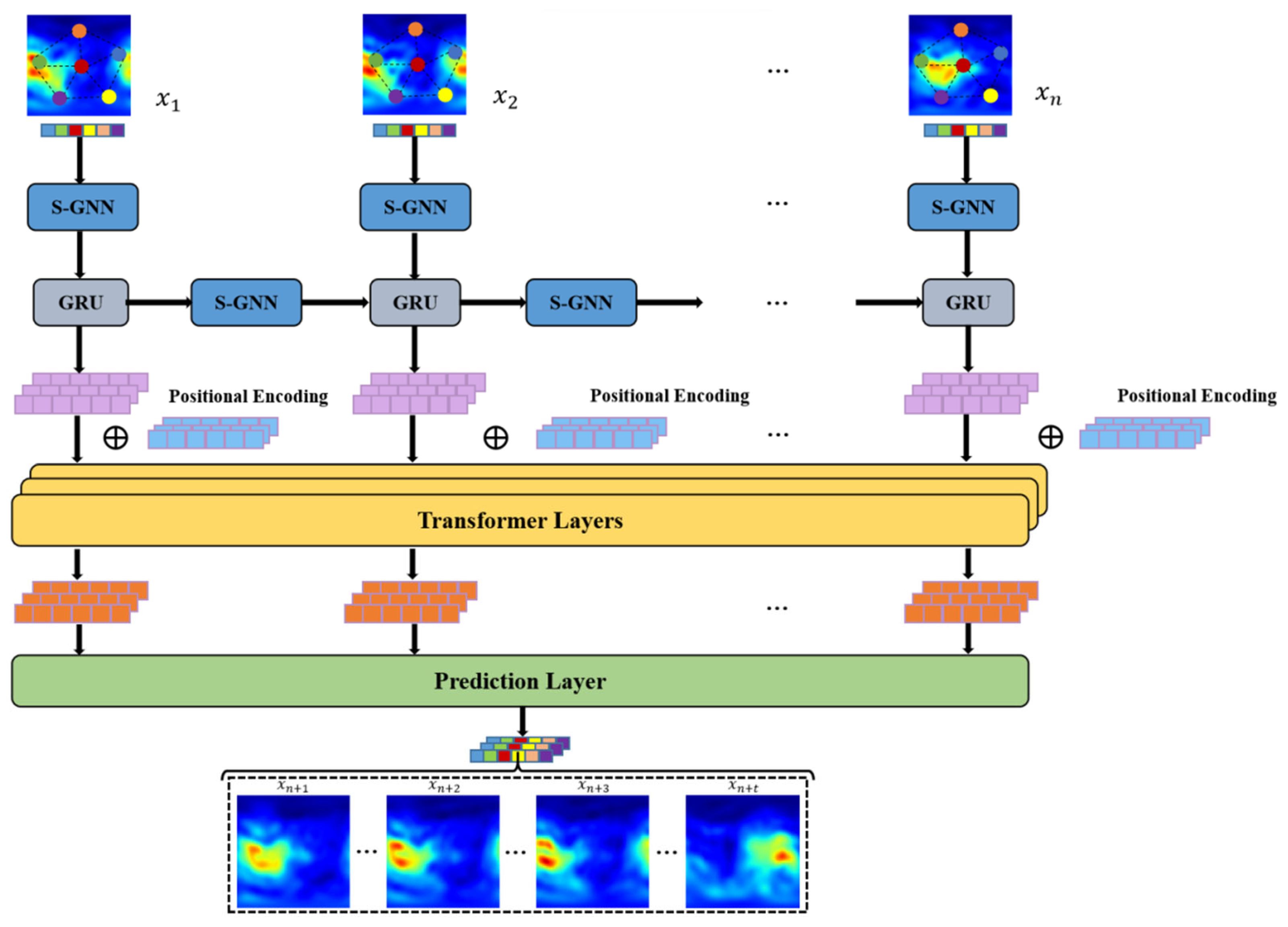
2.2. Methodology
2.2.1. Graph-Based Neural Network Representations
2.2.2. Gated Recurrent Unit for Sequential Data Processing
2.2.3. Attention-Driven Model for Global Dependency Capture
2.2.4. Evaluation Metrics
2.3. Implementation Details
3. Results
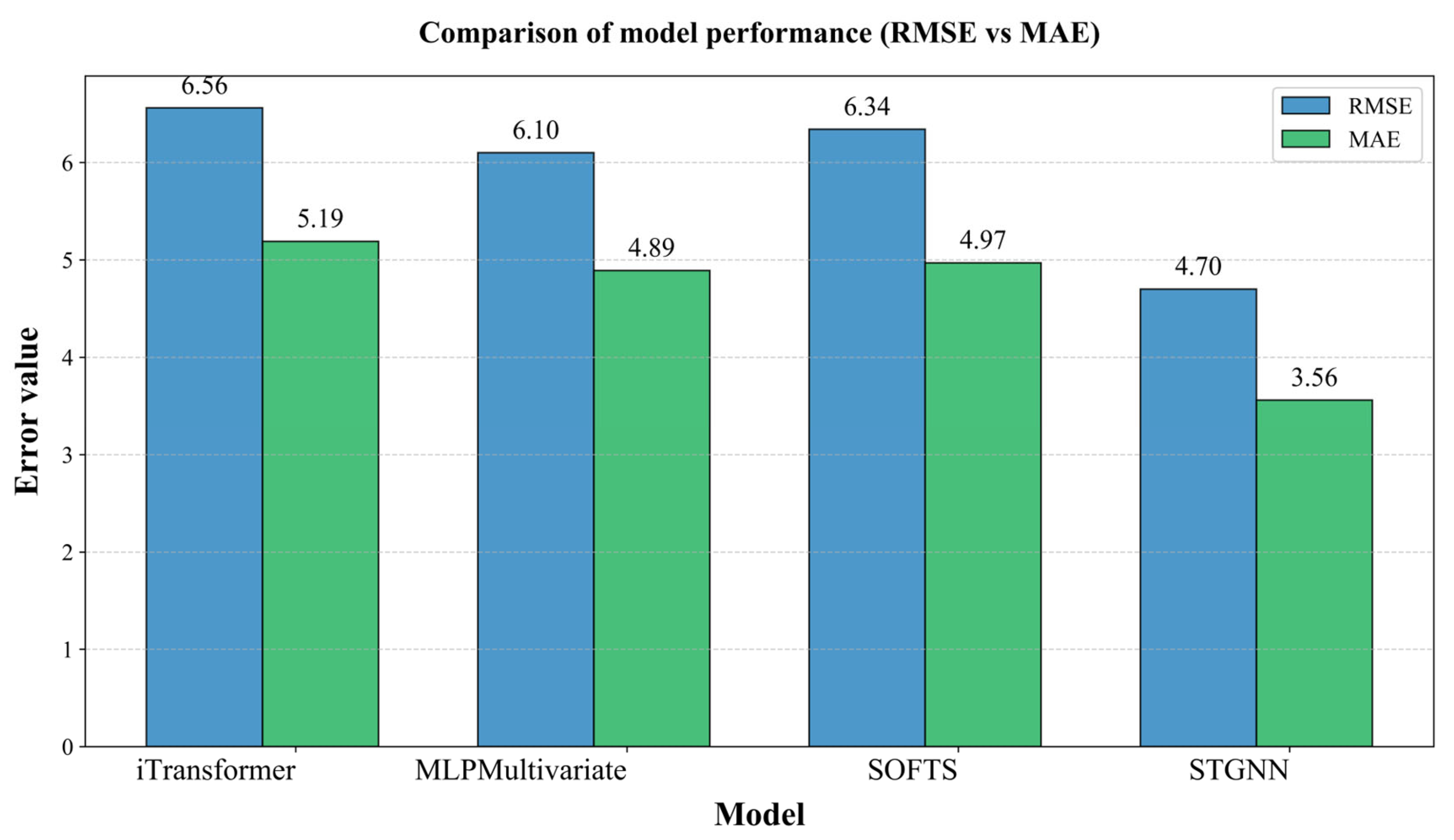
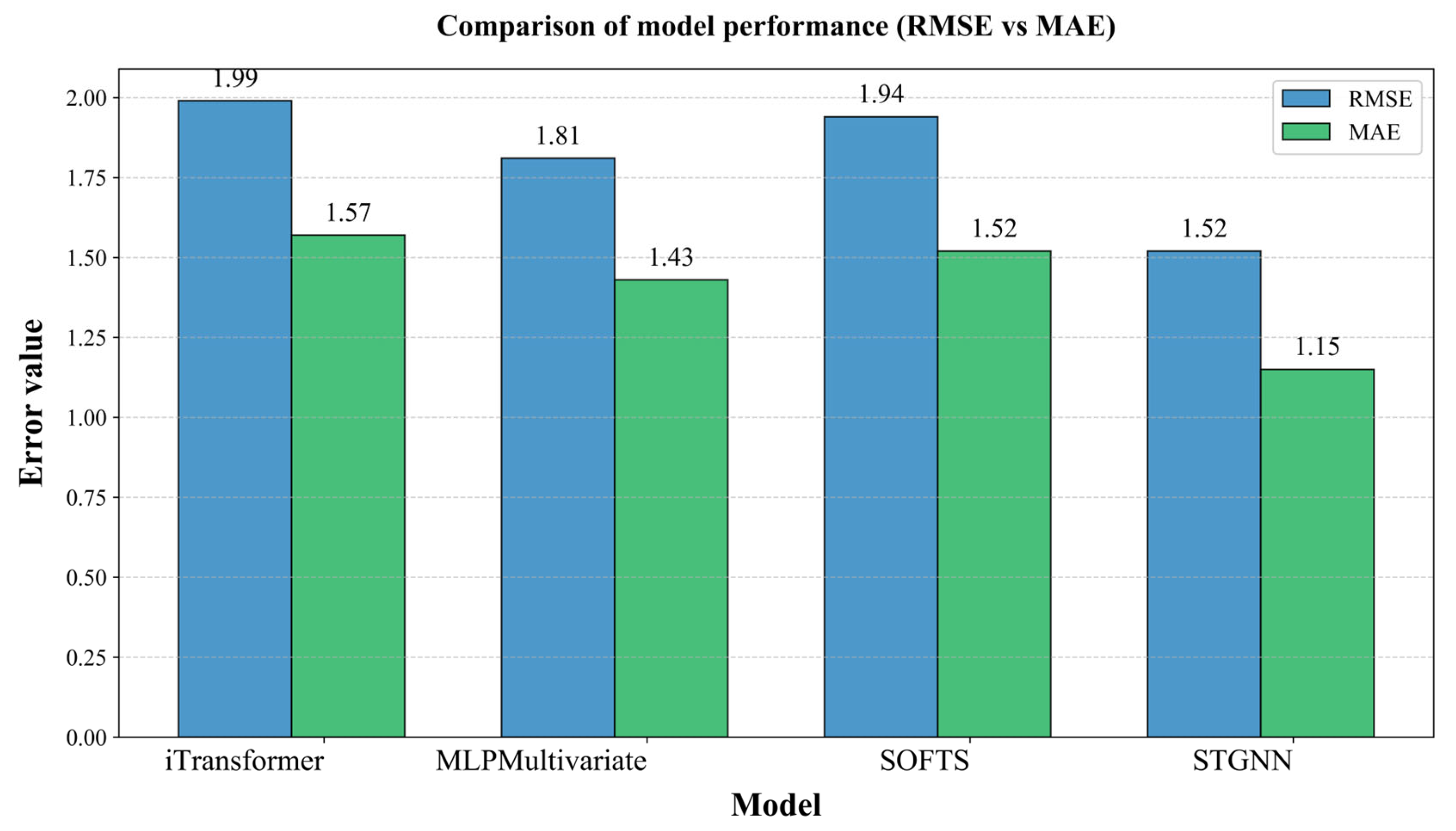
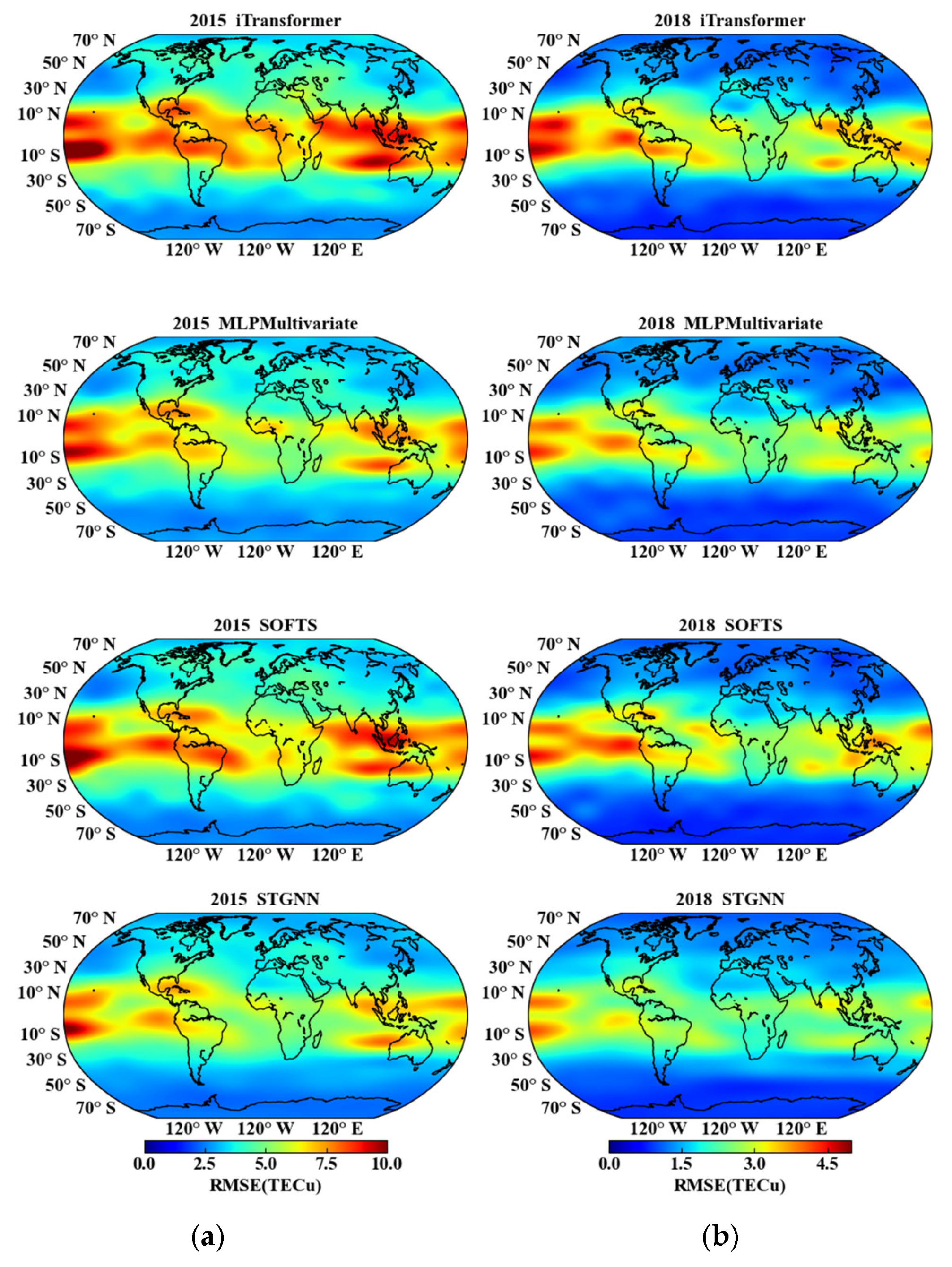
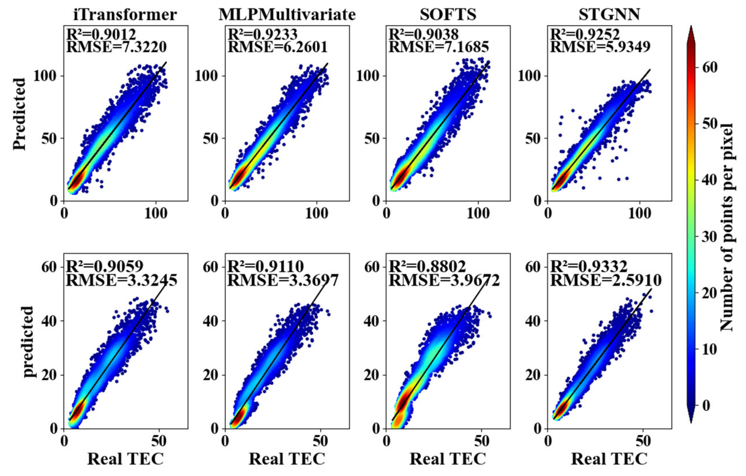
3.1. Performance Under Different Solar Activities
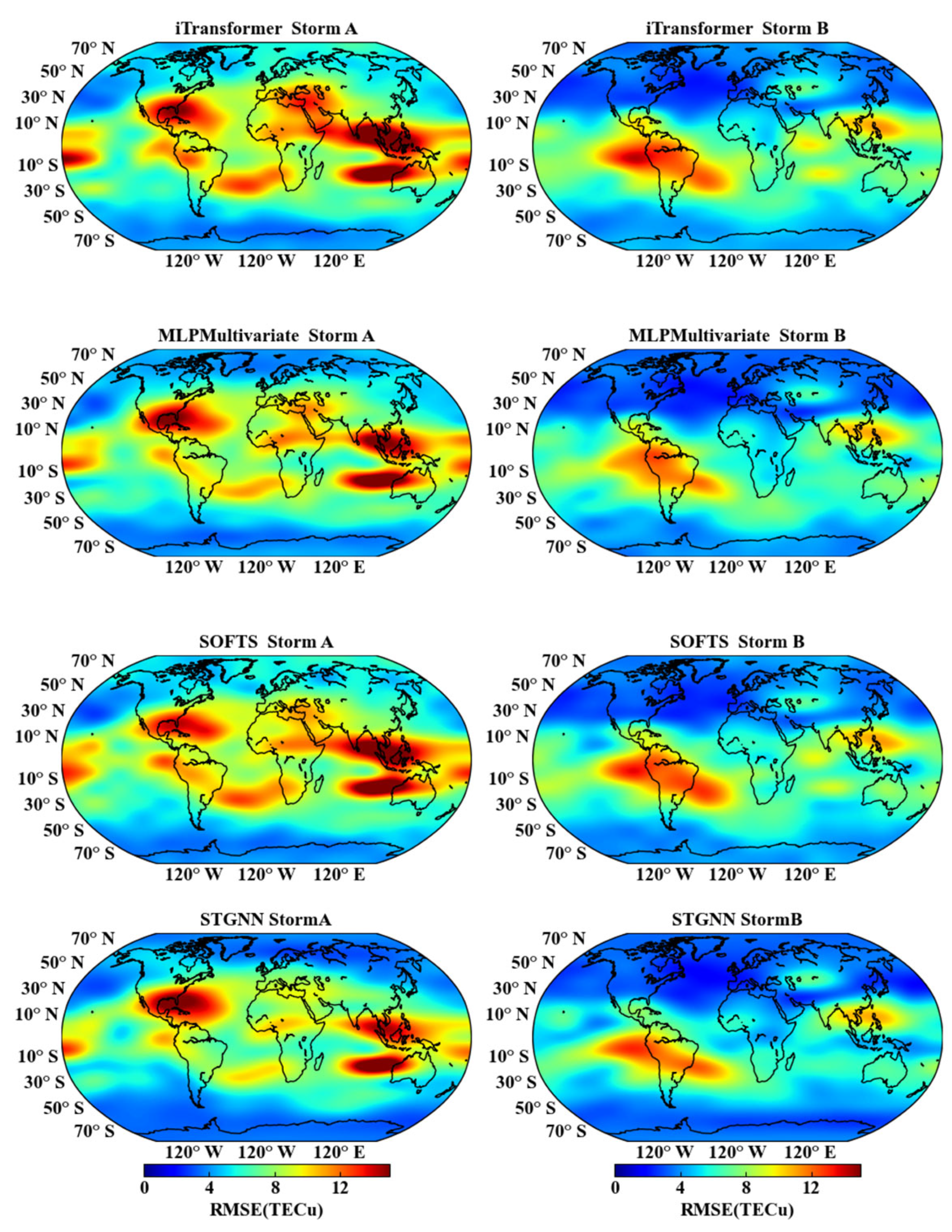
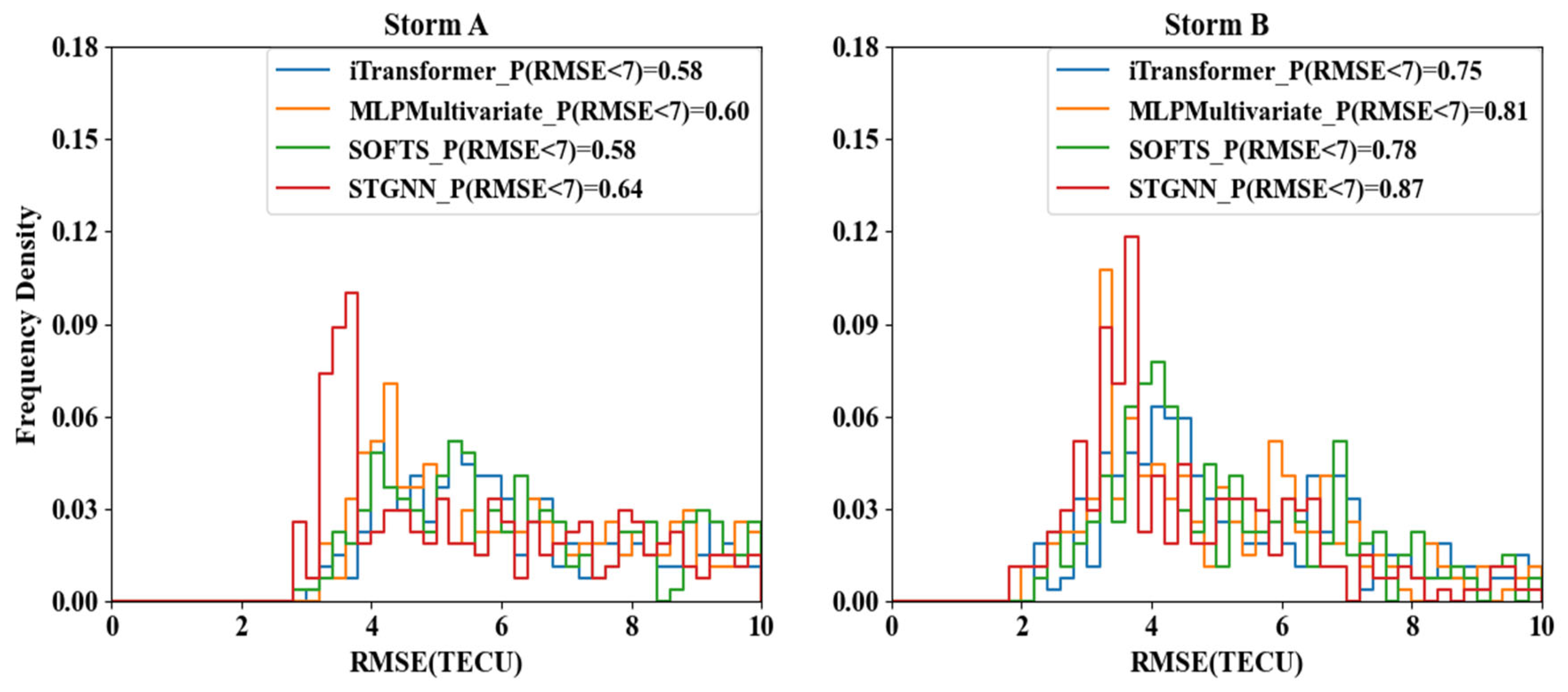
3.2. Performance Under Geomagnetic Storms
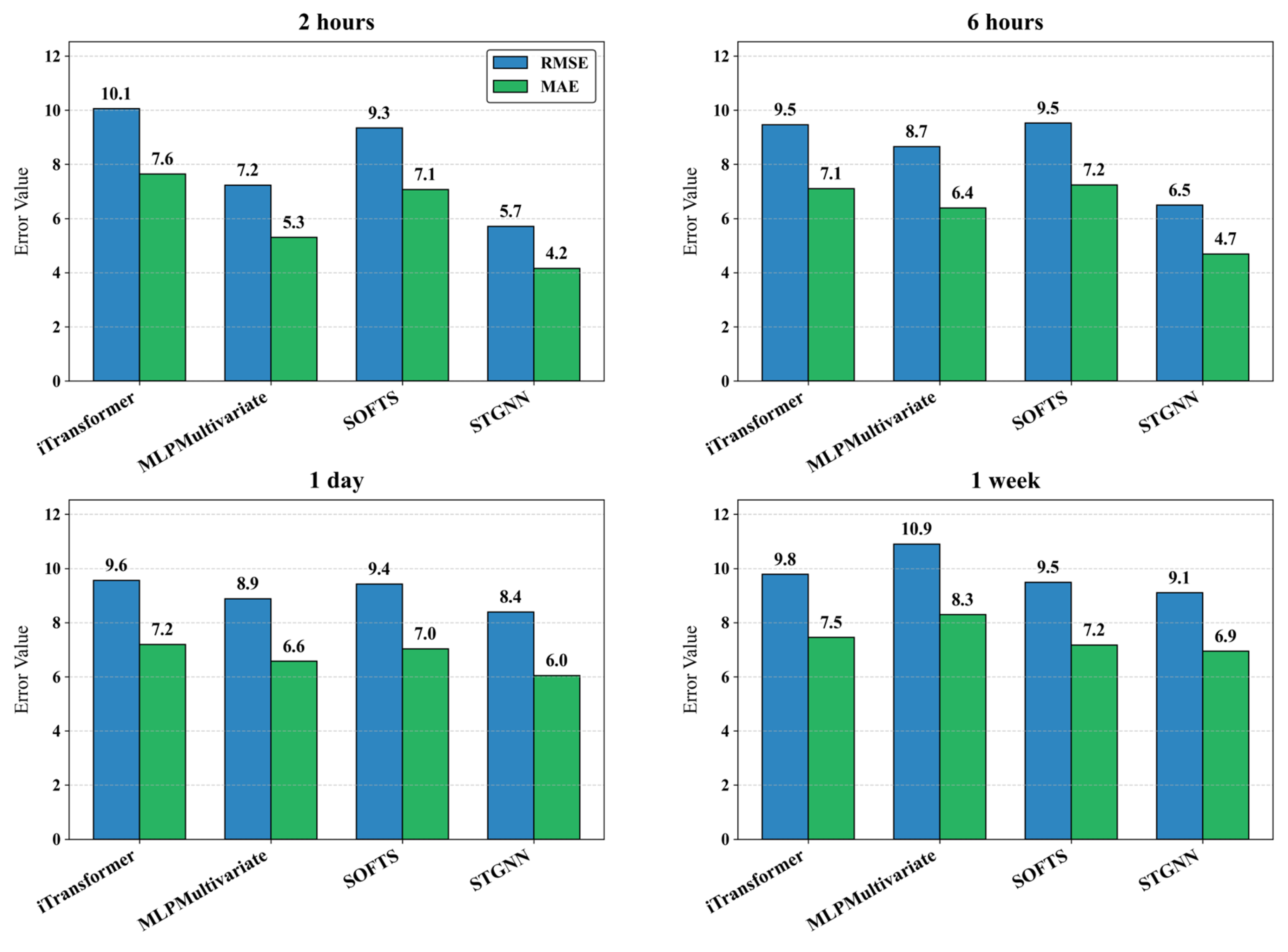
3.3. Performance Under Different Prediction Steps
4. Discussion
5. Conclusions
Author Contributions
Funding
Institutional Review Board Statement
Informed Consent Statement
Data Availability Statement
Acknowledgments
Conflicts of Interest
Abbreviations
| GNSS | Global Navigation Satellite System |
| GNN | Graph Neural Network |
| TEC | Total Electron Content |
| STGNN | Spatio-temporal Graph Neural Network |
| IGS | International GNSS Service |
| GIMs | Global Ionospheric Maps |
| LSTM | Long Short-Term Memory |
| RMSE | Root Mean Square Error |
| GRU | Gated Recurrent Unit |
| MAE | Mean Absolute Error |
References
- Basu, S.; MacKenzie, E.; Coley, W.R.; Sharber, J.R.; Hoegy, W.R. Plasma structuring by the gradient drift instability at high latitudes and comparison with velocity shear driven processes. J. Geophys. Res. 1990, 95, 7799–7818. [Google Scholar] [CrossRef]
- Ratnam, D.V.; Otsuka, Y.; Sivavaraprasad, G.; Dabbakuti, J.R.K.K. Development of multivariate ionospheric TEC forecasting algorithm using linear time series model and ARMA over low-latitude GNSS station. Adv. Space Res. 2019, 63, 2848–2856. [Google Scholar] [CrossRef]
- Yang, Z.; Morton, Y.T.J.; Zakharenkova, I.; Cherniak, I.; Song, S.; Li, W. Global view of ionospheric disturbance impacts on kinematic GPS positioning solutions during the 2015 St. Patrick’s Day storm. J. Geophys. Res. Space Phys. 2020, 125, e2019JA027681. [Google Scholar] [CrossRef]
- Yeh, K.C.; Liu, C.-H. Radio wave scintillations in the ionosphere. Proc. IEEE 1982, 70, 324–360. [Google Scholar]
- Olwendo, J.O.; Cilliers, P.J.; Baki, P.; Mito, C. Using GPS-SCINDA observations to study the correlation between scintillation, total electron content enhancement and depletions over the Kenyan region. Adv. Space Res. 2012, 49, 1363–1372. [Google Scholar] [CrossRef]
- Qi, F.; Lv, H.; Wang, J.; Fathy, A.E. Quantitative evaluation of channel micro-Doppler capacity for MIMO UWB radar human activity signals based on time–frequency signatures. IEEE Trans. Geosci. Remote Sens. 2020, 58, 6138–6151. [Google Scholar] [CrossRef]
- Habarulema, J.B.; McKinnell, L.-A.; Cilliers, P.J. Prediction of global positioning system total electron content using neural networks over south africa. J. Atmos. Sol.-Terr. Phys. 2007, 69, 1842–1850. [Google Scholar] [CrossRef]
- Chen, Z.; Liao, W.; Li, H.; Wang, J.; Deng, X.; Hong, S. Prediction of global ionospheric TEC based on deep learning. Space Weather 2022, 20, e2021SW002854. [Google Scholar] [CrossRef]
- Liu, L.; Morton, Y.J.; Liu, Y. ML prediction of global ionospheric TEC maps. Space Weather 2022, 20, e2022SW003135. [Google Scholar] [CrossRef]
- Xia, G.; Zhang, F.; Wang, C.; Zhou, C. ED-ConvLSTM: A novel global ionospheric total electron content medium-term forecast model. Space Weather 2022, 20, e2021SW002959. [Google Scholar] [CrossRef]
- Xue, K.; Shi, C.; Wang, C. ATS-UNet: Attentional 2-D Time Sequence UNet for Global Ionospheric One-Day-Ahead Prediction. IEEE Geosci. Remote Sens. Lett. 2024, 21, 1002505. [Google Scholar] [CrossRef]
- Zhao, X.; Lu, X.; Quan, W.; Li, X.; Zhao, H.; Lin, G. An Effective Ionospheric TEC Predicting Approach Using EEMD-PE-Kmeans and Self-Attention LSTM. Neural Process. Lett. 2023, 55, 9225–9245. [Google Scholar] [CrossRef]
- Bi, C.; Ren, P.; Yin, T.; Zhang, Y.; Li, B.; Xiang, Z. An informer architecture-based ionospheric foF2 model in the middle latitude region. IEEE Geosci. Remote Sens. Lett. 2022, 19, 1005305. [Google Scholar] [CrossRef]
- Xia, G.; Liu, M.; Zhang, F.; Zhou, C. CAiTST: Conv-attentional image time sequence transformer for ionospheric TEC maps forecast. Remote Sens. 2022, 14, 4223. [Google Scholar] [CrossRef]
- Li, L.; Liu, Y.; Zhou, H.; Yang, K.; Yan, H.; Li, J. Ionformer: A data-driven deep learning baseline for global ionospheric TEC forecasting. IEEE Trans. Geosci. Remote Sens. 2025, 63, 5801012. [Google Scholar] [CrossRef]
- Ren, X.; Yang, P.; Mei, D.; Liu, H.; Xu, G.; Dong, Y. Global Ionospheric TEC Forecasting for Geomagnetic Storm Time Using a Deep Learning-Based Multi-Model Ensemble Method. Space Weather 2023, 21, e2022SW003231. [Google Scholar] [CrossRef]
- Yu, F.; Yuan, H.; Chen, S.; Luo, R.; Luo, H. Graph-enabled spatio-temporal transformer for ionospheric prediction. GPS Solut. 2024, 28, 203. [Google Scholar] [CrossRef]
- Liu, R.; Jiang, Y. Ionospheric VTEC maps forecasting based on graph neural network with transformers. IEEE J. Sel. Top. Appl. Earth Obs. Remote Sens. 2025, 18, 1802–1816. [Google Scholar] [CrossRef]
- Silva, A.; Moraes, A.; Sousasantos, J.; Maximo, M.; Vani, B.; Faria, C. Using Deep Learning to Map Ionospheric Total Electron Content over Brazil. Remote Sens. 2023, 15, 412. [Google Scholar] [CrossRef]
- Gabriel, N.; Johnson, N.F. Using Neural Architectures to Model Complex Dynamical Systems. Adv. Artif. Intell. Mach. Learn. 2022, 2, 366–384. [Google Scholar] [CrossRef]
- Schaer, S.; Gurtner, W.; Feltens, J. IONEX: The IONosphere map exchange format version 1. In Proceedings of the IGS AC Workshop, Darmstadt, Germany, 9–11 February 1998; Volume 9. [Google Scholar]
- Hernández-Pajares, M.; Juan, J.M.; Sanz, J.; Orus, R.; Garcia-Rigo, A.; Feltens, J.; Komjathy, A.; Schaer, S.C.; Krankowski, A. The IGS VTEC maps: A reliable source of ionospheric information since 1998. J. Geod. 2009, 83, 263–275. [Google Scholar] [CrossRef]
- Hernández-Pajares, M.; Juan, J.M.; Sanz, J.; Aragón-Àngel, À.; García-Rigo, A.; Salazar, D.; Escudero, M. The ionosphere: Effects, GPS modeling and the benefits for space geodetic techniques. J. Geod. 2011, 85, 887–907. [Google Scholar] [CrossRef]
- Rovira-Garcia, A.; Juan, J.M.; Sanz, J.; Gonzalez-Casado, G. A worldwide ionospheric model for fast precise point positioning. IEEE Trans. Geosci. Remote Sens. 2015, 53, 4596–4604. [Google Scholar] [CrossRef]
- Li, L.; Liu, H.; Le, H.; Yuan, J.; Wang, H.; Chen, Y.; Shan, W.; Ma, L.; Cui, C. ED-AttConvLSTM: An ionospheric TEC map prediction model using adaptive weighted spatiotemporal features. Space Weather 2024, 22, e2023SW003740. [Google Scholar] [CrossRef]
- Wang, X.; Ma, Y.; Wang, Y.; Jin, W.; Wang, X.; Tang, J.; Jia, C.; Yu, J. Traffic Flow Prediction via Spatial Temporal Graph Neural Network. In Proceedings of the Web Conference 2020, Taipei, Taiwan, 20–24 April 2020; pp. 1082–1092. [Google Scholar]
- Wang, Y.; Duan, Z.; Huang, Y.; Xu, H.; Feng, J.; Ren, A. Mthetgnn: A heterogeneous graph embedding framework for multivariate time series forecasting. Pattern Recognit. Lett. 2022, 153, 151–158. [Google Scholar] [CrossRef]
- Kipf, T.N.; Welling, M. Semi-supervised classification with graph convolutional networks. arXiv 2016, arXiv:1609.02907. [Google Scholar]
- Velicković, P.; Cucurull, G.; Casanova, A.; Romero, A.; Liò, P.; Bengio, Y. Graph attention networks. International Conference on Learning Representations. arXiv 2018, arXiv:1710.10903. [Google Scholar]
- Cho, K.; van Merriënboer, B.; Gulcehre, C.; Bahdanau, D.; Bougares, F.; Schwenk, H.; Bengio, Y. Learning phrase representations using RNN encoder-decoder for statistical machine translation. In Proceedings of the 2014 Conference on Empirical Methods in Natural Language Processing (EMNLP), Doha, Qatar, 25–29 October 2014. [Google Scholar]
- Vaswani, A.; Shazeer, N.; Parmar, N.; Uszkoreit, J.; Jones, L.; Gomez, A.N.; Kaiser, L.; Polosukhin, I. Attention is all you need. arXiv 2017, arXiv:1706.03762. [Google Scholar]


| Year | Latitude | iTransformer | MLPMultivariate | SOFTS | STGNN | ||||
|---|---|---|---|---|---|---|---|---|---|
| MAE | RMSE | MAE | RMSE | MAE | RMSE | MAE | RMSE | ||
| 2015 | Low | 5.348 | 7.121 | 4.636 | 6.230 | 5.106 | 6.815 | 4.017 | 5.561 |
| Middle | 2.975 | 4.082 | 2.739 | 3.805 | 2.914 | 3.999 | 2.340 | 3.398 | |
| High | 2.334 | 3.205 | 2.222 | 3.063 | 2.269 | 3.120 | 1.999 | 2.783 | |
| 2018 | Low | 2.229 | 2.970 | 2.022 | 2.707 | 2.138 | 2.871 | 1.829 | 2.550 |
| Middle | 1.111 | 1.482 | 1.094 | 1.458 | 1.080 | 1.445 | 1.166 | 1.589 | |
| High | 0.783 | 1.037 | 0.869 | 1.128 | 0.772 | 1.024 | 0.822 | 1.092 | |
| L | iTransformer | MLPMultivariate | SOFTS | STGNN | ||||
|---|---|---|---|---|---|---|---|---|
| MAE | RMSE | MAE | RMSE | MAE | RMSE | MAE | RMSE | |
| 2 h | 5.372 | 7.144 | 3.618 | 4.893 | 4.953 | 6.584 | 3.313 | 4.403 |
| 1 day | 5.348 | 7.121 | 4.636 | 6.230 | 5.106 | 6.815 | 4.017 | 5.561 |
| 1 week | 6.176 | 8.220 | 6.551 | 8.573 | 5.867 | 7.804 | 4.195 | 6.255 |
Disclaimer/Publisher’s Note: The statements, opinions and data contained in all publications are solely those of the individual author(s) and contributor(s) and not of MDPI and/or the editor(s). MDPI and/or the editor(s) disclaim responsibility for any injury to people or property resulting from any ideas, methods, instructions or products referred to in the content. |
© 2025 by the authors. Licensee MDPI, Basel, Switzerland. This article is an open access article distributed under the terms and conditions of the Creative Commons Attribution (CC BY) license (https://creativecommons.org/licenses/by/4.0/).
Share and Cite
Chen, Y.; Liu, Y.; Yang, K.; Li, L.; Xiong, C.; Wang, J. Ionospheric Time Series Prediction Method Based on Spatio-Temporal Graph Neural Network. Atmosphere 2025, 16, 732. https://doi.org/10.3390/atmos16060732
Chen Y, Liu Y, Yang K, Li L, Xiong C, Wang J. Ionospheric Time Series Prediction Method Based on Spatio-Temporal Graph Neural Network. Atmosphere. 2025; 16(6):732. https://doi.org/10.3390/atmos16060732
Chicago/Turabian StyleChen, Yifei, Yang Liu, Kunlin Yang, Lanhao Li, Chao Xiong, and Jinling Wang. 2025. "Ionospheric Time Series Prediction Method Based on Spatio-Temporal Graph Neural Network" Atmosphere 16, no. 6: 732. https://doi.org/10.3390/atmos16060732
APA StyleChen, Y., Liu, Y., Yang, K., Li, L., Xiong, C., & Wang, J. (2025). Ionospheric Time Series Prediction Method Based on Spatio-Temporal Graph Neural Network. Atmosphere, 16(6), 732. https://doi.org/10.3390/atmos16060732