Abstract
The SPICAV IR spectrometer aboard the Venus Express orbiter measured spectra of the 1.1 and 1.18 μm atmospheric transparency windows at the Venus night side in 2006–2014. The long-term measurements encompassed the major part of the Venus globe, including polar latitudes. For the first time, the H2O volume mixing ratio in the deep Venus atmosphere at about 10–16 km has been retrieved for the entire SPICAV IR dataset using a radiative transfer model with multiple scattering. The retrieved H2O volume mixing ratio is found to be sensitive to different approximations of the H2O and CO2 absorption lines’ far wings and assumed surface emissivity. The global average of the H2O abundance retrieved for different parameters ranges from 23.6 ± 1.0 ppmv to 27.7 ± 1.2 ppmv. The obtained values are consistent with recent studies of water vapor below the cloud layer, showing the H2O mixing ratio below 30 ppmv. Within the considered dataset, the zonal mean of the H2O mixing ratio does not vary significantly from 60° S to 75° N, except for a 2 ppmv decrease noted at high latitudes. The H2O local time distribution is also uniform. The 8-year observation period revealed no significant long-term trends or periodicities.
1. Introduction
Venus has a dense CO2 atmosphere with very low water content. Whether liquid water has ever existed on Venus remains undetermined. The presence of significant amounts of water in some form in the past is supported by the anomalous isotopic ratio of HDO to H2O. In the lower atmosphere of Venus, the HDO/H2O ratio is approximately 150 times higher than on Earth [1], and above the clouds, it has been measured to be 240 ± 25 terrestrial values [2]. The loss of water from Venus can be attributed to the dissociation of its molecules into oxygen and hydrogen. In the absence of a magnetic field on Venus, the loss of light hydrogen molecules by the atmosphere is significant [3]. Water vapor contained in the lower atmosphere plays a crucial role in the formation of sulfuric acid (H2SO4) clouds, which enshroud the planet by a layer extending from 47 to 70 km. A potential supply of water vapor is volcanic degassing [4,5]. Thus, the study of the abundance and distribution of water vapor in the lower atmosphere allows us to gain a comprehensive understanding of the chemistry and evolution of Venus.
The contribution of water vapor to the present CO2-dominated greenhouse effect on Venus is relatively minor, which is the opposite of what occurs on the Earth. However, H2O absorption bands overlap the transmission of several infrared (IR) transparency windows, regulating the thermal radiation escaping from the surface and deep atmosphere. The atmospheric windows discovered by Allen and Crawford in 1983 [6] are narrow spectral intervals between the strong CO2 absorption bands. They also provide one of the most effective tools to remotely assess the composition of the Venus near-surface atmosphere. Spectral windows at 1.1, 1.18, 1.74 and 2.3 μm coincide with the H2O absorption bands and correspond to thermal emission originating at different altitudes. The 1.1 and 1.18 μm windows allow sensing the surface and the altitudes of 0–15 km. Thermal emission in the 1.74 µm and 2.3 μm windows is formed at 15–30 km and 30–45 km, correspondingly [7]. The Venus transparency windows were observed by several space missions and by means of ground-based astronomy. Water abundance at different altitudes in the atmosphere has been estimated in multiple studies, as summarized in Table 1.

Table 1.
Overview of water vapor measurements in the Venus transparency windows.
Following this corpus of observational evidence, water vapor is well mixed below the clouds. From remote observations, the volume mixing ratio (VMR) of ~30 ppmv (parts per million by volume) was found in the Venus lower atmosphere without any significant vertical evolution. Spectra obtained during the descent of Venera 13 and 14 landers were compatible with two types of H2O profile: (1) a uniform distribution with a VMR of 30 ppmv, (2) a decrease from 30 ppmv at the lower cloud boundary down to 20 ppmv at 10–20 km and then an increase up to 50–70 ppmv below 5 km [28]. It was not possible to distinguish between the two profiles due to experimental uncertainties [28]. Spatial variations of water vapor have not been observed in the 1.18 µm [11,17] and 1.74 µm [17] windows. At higher altitudes, the spatial inhomogeneity of water vapor was detected [17,24], and an anti-correlation between H2O and cloud opacity was suggested [24].
The SPICAV (SPectroscopy for the Investigation of the Characteristics of the Atmosphere of Venus) spectrometer aboard Venus Express observed the Venus transparency windows in 2006–2014 [29]. The very first analysis of the SPICAV dataset was conducted using average spectra from several orbits to improve high-temperature spectroscopy in this range [14]. The study provided the water vapor abundance of 30 +10−5 ppmv [14]. A series of observations in the region of Maxwell Montes during the SPICAV IR campaign was dedicated to investigating carbon dioxide absorption at high temperature and pressure in the transparency windows of 1.1, 1.18 and 1.28 μm [16]. The analysis also constrained the H2O VMR from 25.7+ 1.4−1.2 to 29.4+ 1.6−1.4 ppmv depending on the assumed forward model parameters [16]. An analysis of observations in the 1.28 μm transparency window yielded the most extended monitoring of the optical depth of the Venus cloud layer [30].
This paper is dedicated to the first analysis of the 1.1 and 1.18 µm transparency windows applied to the complete dataset of the SPICAV IR spectrometer. The abundance of water vapor in the deep atmosphere of Venus was studied over a period of 8 years. Observations covering almost the whole night hemisphere are described in Section 2. The data processing algorithm and forward radiative transfer model are considered in Section 3. The retrieved water vapor abundance is reported in Section 4. In Section 5, the results are discussed. The conclusions are presented in Section 6.
2. Observational Dataset
The IR channel of the SPICAV spectrometer operated on board the Venus Express spacecraft from April 2006 to December 2014 [29]. The instrument was based on acousto-optical tunable filter (AOTF) technology, and the spectrum was recorded sequentially by tuning the AOTF to a specific wavelength. The instrument’s spectral range was 0.65–1.7 μm. The tuning capability was also used to define the preferred spectral range and sampling. The incoming light was split into two beams with orthogonal polarizations by the filter and focused onto two Si-InGaAs photodiodes. The silicon and InGaAs sensors were sensitive to radiation in the short-wavelength (0.65–1.05 μm) and long-wavelength (1.05–1.7 μm) spectral ranges, respectively. This study considers spectra in the long-wavelength range, with a spectral resolution of 5.2 cm−1. The detectors had integrated Peltier elements. Measurements with the Peltier coolers switched on are characterized by an increased signal-to-noise ratio (SNR). The thermal emission in the Venus transparency windows is weak, and the spectra were obtained with a long exposure time of 44.8 or 89.6 ms per spectral point. The best SNR for a single spectrum was ~50 for the longest exposure time of 89.6 ms and cooled detectors [29]. Without cooling, the noise-equivalent brightness doubled, all other parameters being equal [29]. For each observation, the signal noise was determined as the standard deviation of the radiance at 1.21–1.24 μm, where the atmosphere is opaque. For measurements in which this spectral interval was unavailable, spectrum uncertainties were scaled to the square root of the exposure time. Radiance calibration accuracy was estimated to be better than 20%. The wavelength was assigned to the spectral point based on the AOTF parameters, and the calibration uncertainty is less than 0.2 nm. The details on the SPICAV IR calibration can be found in Ref. [29].
SPICAV IR had a circular field of view (FOV) with an angular size of 2°. The Venus Express orbit was elongated with a pericenter near the North Pole, and the spacecraft altitude varied from 250 km to 66,000 km. Thus, the SPICAV footprint diameter varied from 9 km to 2300 km from northern to southern latitudes, and the observations of the Southern Hemisphere had lower spatial resolution. The achieved spatial coverage is shown in Figure 1.
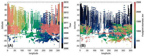
Figure 1.
Spatial distribution of the 1.1 and 1.18 µm transparency window observations analyzed in this study. (A) Color indicates the year of the individual measurements. (B) Color codes for the diameter of the SPICAV IR footprint in kilometers.
The instrument observed the Venus transparency windows at 1.0, 1.1, 1.18, 1.28 and 1.31 μm. Due to the long exposure time of one spectral point, the footprints of different transparency windows are spatially separated, in particular in the Northern Hemisphere. To improve the data concurrency, we limit the analyzed spectral range to 1.06–1.21 μm, covering the 1.1 and 1.18 μm windows to study the water vapor content in the lower atmosphere of Venus.
Closer to the terminator, a footprint may capture a fraction of scattered solar light resulting in contamination with a continuous background. This contribution was removed from the spectrum by linear interpolation between the 1.06–1.07 μm and 1.205–1.24 μm intervals, where the atmosphere of Venus is opaque. Strongly contaminated measurements for which the scattered light spectrum cannot be reproduced by linear interpolation were discarded. The selected observations overlap the Venus solar local times from 18:20 to 5:40. During eight years of the Venus Express mission, observations covered almost the entire latitude range from 84° S to 84° N. Due to Venus’ slow rotation, the longitude coverage depends on the year of the space mission (Figure 1A). The total dataset consists of more than 2600 observation sessions, corresponding to approximately 27000 spectra.
3. Methods
3.1. Radiative Transfer Model
A radiative transfer model including multiple scattering is used to synthesize transparency-window spectra. The model was successfully implemented to reproduce the SPICAV IR spectra of the 1.28 μm transparency window, thereby enabling the retrieval of the total cloud optical depth [30]. It is based on the DISORT 4.0.99 program package [31,32], with 16 streams implementing the discrete ordinate method in a pseudo-spherical geometry to solve the radiative transfer equation. The pseudo-spherical approximation is necessary when the emission angles exceed 60°, which is the case for ~1% of the analyzed dataset.
The a priori atmosphere is defined by vertical profiles of temperature and optical properties (optical depth of computational layers, single scattering albedo and Legendre series expansion of the scattering phase function). The upper boundary is set at 100 km above the reference sphere, and the atmosphere is divided into discrete homogeneous 1-km layers. For altitude profiles of temperature, pressure and density, we use the Venus International Reference Atmosphere (VIRA) [33]. The surface temperature is assumed to be equal to the atmospheric temperature at the altitude of local elevation. Average elevation within the SPICAV IR footprint is derived from the Magellan topography map [34,35].
The Venus cloud layer is modeled following the Ref. [36] approach. The aerosol particles are represented by four modes (1, 2, 2′ and 3) of log-normal size distribution. Each mode is characterized by the effective radius of 0.3, 1.0, 1.4 and 3.65 μm and the dimensionless dispersion of 1.56, 1.29, 1.23 and 1.28, respectively [7,36]. The imaginary part of the refractive index is less than 6 × 10⁻⁶; thus, the absorption by cloud aerosol particles is negligible. The real part of the refractive index has a weak dependence on the wavelength, and its values are similar for different acidities of H2SO4 solution in the 1.06–1.21 μm spectral range. The cloud droplets’ concentration is fixed to 75%. Aerosol extinction, single-scattering albedo and the Legendre expansion coefficients of the scattering phase function are computed for each mode using the Lorenz–Mie code for electromagnetic scattering of light by spherical particles [37].
The outgoing radiance within the 1.1 and 1.18 μm transparency windows forms at 0–15 km (Figure 2A). The deep atmosphere has a large thermal inertia preventing any diurnal variation of temperature. Based on the multispectral images by the Near-Infrared Mapping Spectrometer on board the Galileo spacecraft, horizontal temperature variations were also constrained to ±2 K on the Venus night side [38]. Another factor affecting the radiance in the spectral windows is the surface emissivity. Reducing the emissivity from 0.95 to 0.4 results in 16% and 15% dimming in 1.1 and 1.18 μm transparency windows, respectively (Figure 2C). The absolute emissivity of the Venus surface in the near-infrared (NIR) range is difficult to assess [39]. Nevertheless, its variation over the surface was observed and linked to the different geological areas: tesserae, basaltic plains or recent lava flows [40]. Generally, the decrease in emissivity is associated with higher elevations [38,40]. In this analysis, the surface emissivity of 0.95 was assumed. The sensitivity of the retrieved water vapor volume mixing ratio to this parameter is discussed in Section 3.5.
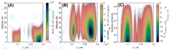
Figure 2.
(A) Radiance increment caused by a temperature rise of 1 K within a 1-km layer centered at a given altitude. (B) Radiance decrease caused by a H2O VMR increase by 1 ppmv within a 1-km layer centered at a given altitude. (C) Relative radiance attenuation due to surface emissivity reduction. Synthetic spectrum with the emissivity value of 0.95 is a reference.
The forward model includes absorption by the CO2, H2O and HDO molecules. The core of the H2O absorption band located at 1.12–1.16 μm falls in between the two considered spectral windows at 1.1 and 1.18 μm. The sensitivity of outgoing radiance to the H2O mixing ratio may be evaluated as the radiance change induced by the water vapor VMR increases by 1 ppmv at each wavelength (Figure 2B). The sensitivity for the whole H2O band extends from 7 to 30 km with a peak at 16 km. Within the transparency windows, the sensitivity to the H2O VMR peaks at 10 km and extends from 4 to 22 km. The limits of model sensitivity to H2O are defined as a full width at half maximum of the obtained radiance change profile. Consequently, the resulting spectrum is weakly sensitive to any potential gradient within the range of 0–5 km. In the forward model, H2O is therefore assumed to be uniformly mixed under clouds.
HDO should contribute to at least 7% of gaseous absorption in the 1.18 μm window [14,16]. We do not attempt to retrieve it and include HDO in the model with the D/H ratio fixed to 127 times the terrestrial value [16,41], or 1.98 × 10⁻². The stoichiometric ratio [HDO]/[H2O] equals 2 D/H [41].
The carbon dioxide mixing ratio is set to 0.965. The CO2 Rayleigh scattering cross-section is calculated according to [42,43].
3.2. Calculation of CO2 and H2O Absorption
Modeling gaseous absorption at high pressure and temperature requires considering several factors. These include the contribution of numerous weak lines, the description of the wings and the CO2 absorption continuum. Additionally, line parameters at high temperature must be taken into account.
In order to account for weak absorption lines with the spectral line intensity down to 10−45 cm−1/(molecule cm−2), an updated carbon dioxide line list from the HITEMP spectroscopic database [44] is used. The absorption of H2O is modeled based on the BT2 line list [45] with CO2-pressure broadening coefficients [46]. The VTT line list [47] with CO2-pressure broadening coefficients [48] is used to compute the HDO absorption.
A deviation of a spectral line wings from the Lorenz profile at high pressure and temperature introduces an additional uncertainty in the determination of gaseous absorption. For the CO2 lines, the absorption due to their far wings is smaller than that described by the Lorentzian profile (the sub-Lorentzian line shape). Conversely, the super-Lorentzian line shape is characteristic for water vapor. In this study, we evaluate three different approaches to describe the far wings of the CO2 and H2O absorption lines, named Model 1, 2 and 3. As demonstrated below, the line shape model affects the retrieved value of the water vapor content in the deep Venus atmosphere.
Model 1 follows the absorption line shape representation from Refs. [14,16], with the sub-Lorentzian profile for CO2 and the Voigt profile for H2O. An example of CO2 and H2O cross-sections computed at 10 km (44.2 atm, 651 K) using Model 1 line shape approximation is presented in Figure 3.
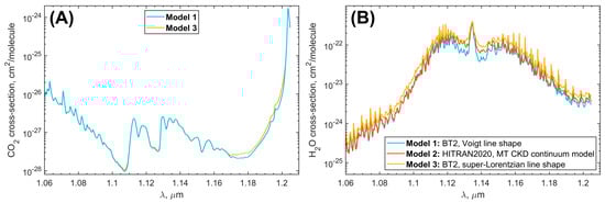
Figure 3.
CO2 (A) and H2O (B) cross-sections computed at 10 km (44.2 atm, 651 K) for different approximations of gaseous absorption in far wings. Blue color corresponds to CO2 and H2O cross-sections computed using line profile approximations of Model 1 [14,16]. The red curve shows the H2O absorption cross-section defined by Model 2 [49]. Yellow color designates CO2 and H2O cross-sections computed using line profile approximations of Model 3 [10,50].
Model 2 follows the same CO2 line shape as Model 1. For H2O, the MT_CKD (Mlawer–Tobin_Clough–Kneizys–Davies) water vapor continuum model is used [49]. The MT_CKD provides a superimposed absorption in the H2O line wings besides the ±25 cm−1 interval from the line center. The H2O foreign continuum is developed and experimentally verified for the Earth atmospheric conditions in the range of 8100–8500 cm−1 [51].
The MT_CKD model is integrated into the HITRAN molecular spectroscopic database [49]. In Model 2, we use HITRAN2020 [52], unlike the BT2 line list [45] for Model 1, to compute the absorption in the line center within ±25 cm−1 and to subtract the line “pedestal” at 25 cm−1 for the correct MT_CKD model implementation (see Ref. [49]). The MT_CKD model and HITRAN2020 are developed for the Earth-atmosphere conditions, and therefore, the broadening by air pressure is implied. For Venus, the air-broadened half widths (γair) of HITRAN2020 are multiplied by a coefficient of 1.5, as the mean adjustment coefficient applied in [53]. In Model 2, the resulting absorption in the core of the H2O band is higher than in Model 1, altering the spectrum in the 1.12–1.15 μm range (Figure 3B).
The formulation of the MT_CKD H2O continuum model is close to the single line shape correction approach. This differs from the CO2 continuum proportional to the squared atmospheric density, as discussed below. To prevent any potential ambiguity between these two terms, we will refer to the MT_CKD H2O continuum model as “H2O far-wings correction by the MT_CKD model”.
Model 3 [10] provides the highest absorption for both CO2 and H2O among the three approaches. The CO2 spectral shape in Model 3 is wider than in Model 1, providing more absorption in the far wings, and it mainly influences the spectral shape of the 1.18 μm transparency window (Figure 3). Even though Model 3 has been implemented for the analysis of Venus transparency windows [10], the H2O line wings are described by the super-Lorentzian profile broadened by air [50]. Nevertheless, the resulting H2O absorption is higher in the whole spectral interval 1.06–1.21 μm (Figure 3).
In the calculations, the absorption line wings extend from the center of a line at 250 cm−1 for CO2 and 180 cm−1 for H2O (Model 1 and 3) and HDO. The Voigt line profile is used for HDO.
At high temperatures and pressures, a superposition of collision-induced transitions, far wings of strong CO2 bands and suspected absorption by molecule dimers form a carbon dioxide continuum absorption proportional to the squared density described by so-called binary absorption coefficient α [30,54]. For the 1.1 and 1.18 µm transparency windows, α was constrained as (0.29–0.66) × 10−9 cm−1amagat−2 and (0.30–0.78) × 10−9 cm−1amagat−2, respectively, obtained when computing the CO2 lines using the “High-T” spectral database [16]. The CO2 continuum was also estimated from the laboratory measurements in the 1.18 μm spectral range as α ~ 0.3 × 10⁻⁹ cm−1amagat−2 [16,55] using the “High-T” spectral database [7,14] to compute the line absorption. We recomputed the laboratory-determined value for the HITEMP spectroscopic database, which includes more spectral lines than “High-T”, and the line shape parameters of Model 1, 2 and 3. We fixed the CO2 continuum coefficient in both windows to a value of 0.3 × 10⁻⁹ cm−1amagat−2 for Models 1 and 2 and of 0.1 × 10⁻⁹ cm−1amagat−2 for Model 3. One amagat density unit corresponds to 2.687 × 10¹⁹ molec/cm3.
3.3. Fitting Algorithm and Variable Parameters
The inversion of the measured spectra starts with removing the background, which is formed due to scattered solar light or remaining dark current signal. The background level is low yet comparable to the signal in the water vapor absorption band (1.1–1.6 μm). The signal in the ranges of 1.06–1.07 μm and 1.205–1.24 μm is approximated by a linear function and subtracted from the spectrum. Then, the spectrum is fit to a model with two variable parameters.
The cloud optical depth is highly variable, affecting the radiation in the whole 1.06–1.21 μm spectral range. Following the approach of Ref. [30], the intensity variations in the spectral windows due to cloud opacity are fitted by adjusting a scaling factor applied to the vertical profiles of aerosol particles’ number densities of modes 2, 2′ and 3. The parameters of each mode remain fixed, as described in Section 3.1.
The second variable parameter of the radiative transfer model is the volume mixing ratio of water vapor, which is constant with altitude. An overview of all the model parameters is provided in Table 2.
Table 2.
Summary of parameters and methods used in the radiative transfer model.
Transparency-window spectra are fitted to the measurements using a look-up table, where the outgoing Venus radiance is calculated for discrete values in a four-parameter space: 40–240% for the aerosol particle number density scaling factor with a 20% step, and 16–40 ppmv for the H2O VMR with one ppmv step. The spectra are computed on a wavelength grid with a step of 0.1 cm−1 for various initial heights and emission angles. Surface heights vary from −2 to 10 km with a 1 km increment. The emission angles are considered from 0° to 80° with a step of 10°. The spectra are then convolved using the SPICAV IR point spread function [30].
Large footprint observations can be affected by atmospheric curvature or spatial inhomogeneity. We assume that the cloud opacity is constant within the FOV, and the topography elevation is equal to the mean height of the area. To account for atmospheric curvature, the model is averaged along the spread of emission angles defined by the spacecraft’s distance from Venus and the angular size of the instrument’s FOV [30]. The reduced χ2-value (i.e., the χ2-value divided by the degrees of freedom) of the experimental and modelled spectra, computed by multilinear interpolation over the look-up table, is minimized by varying parameters with the simplex algorithm [57].
A comparison of the model and an observed spectrum shows that the spectral shape of the 1.18 μm transparency window depends on the CO2 line profile approximation (Figure 4). The discrepancy can be systematically observed in the 1.18–1.2 μm range if the spectrum noise level is below 0.005 W/(m2 μm sr). It is particularly pronounced when successive spectra are averaged, thereby reducing the noise level in the data (Figure 4). For the average spectrum in the entire spectral range, the χ2-value for Model 3, i.e., for the widest absorption line profiles, is reduced by 30% (Figure 4A). In contrast to the 1.18 μm window, the 1.1 μm transparency window is accurately characterized by the three models.
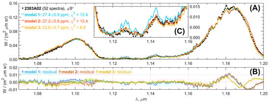
Figure 4.
(A) Mean of 52 spectra measured during the #2383A02 orbit (29 October 2012, latitudes of 14.9° S–33.0° N, longitude of 44.1°, local time of 1H20) fitted by the radiative transfer model computed for the CO2 and H2O line profiles of Model 1, 2 and 3. Surface emissivity is set to 0.95. (B) Residuals of the Models 1, 2 and 3. (C) Same as Panel A for the spectral range of 1.11–1.16 μm. The Panel A legend indicates the emission angle value.
The line shapes of Model 2 and 3 provide stronger absorption in the core of the H2O band, leading to a reduction on the resulting χ2-value. The χ2-value computed within 1.11–1.16 μm (Figure 4C) equals 2.95, 0.88 and 0.95 for H2O line shapes by Model 1, 2 and 3, respectively. Therefore, the theoretical spectrum in the core of the H2O absorption band provides a better representation of the experiment when incorporating the H2O far-wings correction, i.e., Model 2 and 3.
3.4. H2O VMR Retrieval Uncertainties
The H2O VMR retrieval uncertainties are defined by (1) the experiment errors and (2) the uncertainty of the background elimination. To estimate the propagation of the background uncertainty to the retrieved H2O VMR, we consider so-called “spot-tracking” observations. SPICAV IR has conducted ~1000 sessions where four or more sequential spectra are obtained while observing the same location from the distant branch of the orbit, i.e., the footprint (“spot”) shift is negligible. One spectrum is recorded for about 1 min, and the whole observational session lasts several minutes. This timescale is small enough to neglect water vapor or cloud variations and associate a spread of the values to the algorithmic and experimental uncertainties. The obtained spread of the retrieved values was compared with the H2O VMR retrieval uncertainties, computed from the covariance matrix for the residual χ2-function. The computed uncertainties are in good correspondence with the STD of the H2O VMR in “spot-tracking” observations. Therefore, the obtained scatter of values (Section 4) represents the uncertainty rather than the variability of water vapor.
3.5. Surface Emissivity Uncertainty
The emission in the 1.1 and 1.18 μm windows is also sensitive to the surface emissivity (Figure 2C) whose value is poorly known in the NIR range. The Magellan radar mission measured microwave emissivity of ~0.85, on average, with variations from ~0.35 at Maxwell to ~0.95 northeast of Gula Mons and other locations [58]. The lowest emissivity appeared in elevated areas [58]. Surface albedo measurements on the Venera 9 and 10 landers provided a value of emissivity 0.85–0.9 at 0.9 μm [54,59]. In our basic model, a constant surface emissivity of 0.95 is assumed.
Poorly constrained emissivity may affect the retrieved H2O VMR, introducing ambiguity in the contribution of surface (emissivity) and atmospheric (CO2-continuum) radiation. Thus, we investigated how sensitive the VMR retrievals are to this parameter, assuming the nominal (0.95) and reduced (0.4) emissivity.
For the individual spectra, both emissivity values show the same quality of fit. Examples of the spectra are presented in the Supplementary Materials, Figures S1.1–S1.3. For measurements with lower noise, χ2 is 10% larger for the emissivity of 0.4. The systematic non-zero residual at 1.18–1.2 μm in these observations also increases by 10%. Thus, the data fitting for a lower emissivity did not show significant improvement.
Emissivity is connected to another variable parameter, the scaling factor of aerosol number density, and, accordingly, the optical depth of the cloud layer. A decrease in emissivity by 0.65 results in an average decrease in optical depth at Δτ = 4. In contrast, the increase in the H2O VMR is below a standard deviation of the obtained mean values. Distributions of retrieved H2O mixing ratios obtained for two values of surface emissivity are presented in the Supplementary Materials, Figure S2.
The formal inclusion of surface emissivity as a variable parameter into the minimization problem showed a correlation between the scaling factor of aerosol number density and the emissivity at 1.06–1.21 μm of ≥ 0.9, while the cloud scaling factor and H2O VMR are uncorrelated. Further refinement of this parameter is beyond the scope of this study.
4. Results
4.1. Water Vapor Volume Mixing Ratio at Altitudes of 10–16 km
The H2O volume mixing ratio in the Venus lower atmosphere was retrieved from the nadir spectra obtained over 8 years, from April 2006 to December 2014, by SPICAV IR/VEx. The radiative transfer model was computed for three approximations of far wings of the CO2 and H2O absorption lines (Table 2). The weighted average of the H2O VMR over the ensemble of all observations, using the measurement error as weight, is presented in Table 3. The standard deviation of the values is ~1 ppmv for all the absorption line approximations.
Table 3.
Weighted mean of the water vapor volume mixing ratio in the lower atmosphere of Venus retrieved using different approximations of the CO2 and H2O absorption line shape and surface emissivity values of 0.95 and 0.4. Radiative transfer model details can be found in Table 2.
The error bars of the H2O VMR were computed from the covariance matrix for the residual range between 0.5 to 5.7 ppmv, with an average value of 1.1 ppmv. Elevated values of water vapor mixing ratio, exceeding the mean value by 3 σ, are retrieved with error bars higher than 1.5 ppmv. The values and their associated uncertainties depend on the H2O line shape approximation, the signal noise and any residual background signal. It has been found that higher noise levels generally result in slightly lower VMRs, since the residual background signal is also determined with the increased uncertainty. When considering spectra with signal uncertainties below 0.006 W/(m2 μm sr), the variability of the H2O VMR is reduced to ±15% of the mean. Such filtering results in a slight increase in mean values to 27.4 ± 0.9, 27.1 ± 0.9 and 23.7 ± 0.8 ppmv for the CO2 and H2O absorption line shape approximations of Model 1, 2 and 3, respectively. The VMR error bars are close to the obtained standard deviation, strongly suggesting that there is no significant variability of water vapor at 10–16 km.
The line wing approximation introduces a systematic uncertainty to the results. This uncertainty exceeds both the H2O VMR error bars and the resulting standard deviation of the values (Table 3). A decrease in emissivity in the model weakly influences the retrieved H2O VMR, resulting in its systematic increase within the error bars (Table 3).
4.2. H2O Spatial Distribution
The latitudinal profile presented in Figure 5 was averaged, taking into account the footprint size (Figure 1). The zonal mean of the water vapor VMR does not vary significantly from 60° S to 70° N. At latitudes above 60° S, the VMR zonal mean exhibits a decrease of 2 ppmv. SPICAV IR was only capable of observing these latitudes from a large distance, resulting in a footprint diameter of 1000–2000 km (Section 2).
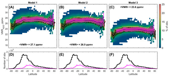
Figure 5.
(A–C) Water vapor volume mixing ratio with respect to latitude. Values were retrieved using the CO2 and H2O absorption line approximation of Model 1 (A), Model 2 (B) and Model 3 (C), presented in detail in Table 2. Color represents the percentage of retrievals in the corresponding VMR bin of 0.5 ppmv relative to all retrievals in the same latitudinal bin of 3°. The black line is the latitudinal distribution of the H2O VMR weighted mean in the latitudinal bin. The magenta line is a similar distribution for a set of values obtained in spectra with signal noise less than 0.006 W/(m2 μm sr) and a footprint diameter smaller than 1000 km. Error bars represent a standard deviation within one bin. (D–F) Histogram representing the number of values in one latitudinal bin. Black color corresponds to the latitudinal distribution based on the whole set of observations. Pink color shows distribution of measurements with signal noise < 0.006 W/(m2 μm sr) and a footprint diameter < 1000 km.
The obtained H2O latitude behavior does not change for different approximations of gaseous absorption line shapes. The radiative transfer model accounts for the atmospheric curvature, i.e., the variation in emission angles across the SPICAV IR FOV. Other parameters are set as uniform across the footprint, including the surface elevation. With this assumption, there is no correlation between the retrieval parameters and the footprint diameter or the emission angle (linear correlation coefficient of 0.01). Consequently, the radiative transfer model demonstrates robust performance. Distant observations of latitudes above 60° S are characterized by the elevated noise level—greater than 0.007 W/(m2 μm sr)—resulting in increased VMR error bars >1 ppmv. Similarly, a decrease of 2 ppmv is obtained at latitudes of 75–85° N, where observations had noise greater than 0.006 W/(m2 μm sr). As previously discussed, an increase in spectrum uncertainty can result in a lower VMR. Moreover, these latitudinal intervals are less densely sampled (Figure 5D–F), and observations above 75° S have an error of ~1.5 ppmv because the detector cooling was turned off. The zonal mean of the water vapor VMR, computed for observations with a footprint diameter less than 1000 km and a noise level below 0.006 W/(m2 μm sr), demonstrates no latitude dependence at latitudes from 60° S to 75° N (Figure 5, magenta color). This sampling does not provide further details on a VMR decrease at polar latitudes.
The observations collected over 8 years allow us to compile the geographic distribution of water vapor in the lower atmosphere of Venus. When the data is binned by 10° of latitude and 10° of longitude, observations cover 63% of the Venus globe (Figure 6). The geographic distribution was computed for the mean of the three outputs obtained using Models 1, 2 and 3 (Figure 6A). The geographic distribution of the H2O VMR is nearly uniform. The latitudinal decrease at polar latitudes is evenly distributed along the longitude in the Southern Hemisphere. Few features, which might be associated with the topography, either belong to the poorly sampled Northern Hemisphere or remain within the STD. The standard deviation calculated over a map bin (Figure 6C) is in the range of 0.8–1.0 ppmv almost for the entire map. This value is in good correspondence with the STD for the ensemble of data, corroborating the uniform distribution of H2O in the lower atmosphere.
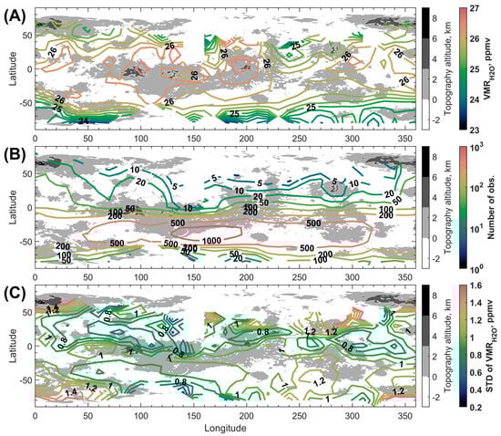
Figure 6.
(A) Geographic distribution of the weighted mean value of H2O VMR obtained on a grid with a 10° latitude and 10° longitude step. (B) Statistics of observations in each 10° latitude–longitude bin. (C) STD of H2O VMR in each 10° latitude–longitude bin. Contour plots are overlaid on the Venus topographic map obtained by the Magellan space mission [34,35].
Spectra obtained during the descent of Venera 13 and 14 landers exhibited nearly equal goodness of fit, assuming either the uniform H2O VMR profile (30 ppmv) or the H2O VMR increase from 20 ppmv at 5 km to 100 ppmv at the surface [28]. Thereafter, no further confirmation of the water vapor vertical gradient near the surface was obtained. Transparency window spectra have poor sensitivity for this altitude range, while the best sensitivity is achieved at 10–16 km. In order to address any possible altitude dependence, we considered a correlation between the retrieved values and corresponding local elevations [34,35] to find a linear correlation coefficient of 0.1. The mean geographic VMR distribution shows a 0.4 ppmv increase in VMR over Ovda Regio (longitude of 75–105°, latitude of 10° S–8° N, maximum elevation of 5 km) and Atla Regio (latitude of 10° S–25° N, longitude of 180–215°, maximum elevation, i.e., Maat Mons, of 8 km) (Figure 6A). This increase is, however, below significance level, since the STD of the values in one bin is 0.8–1.0 ppmv (Figure 6C). Therefore, no persistent correlation with the relief could be established due to the experimental uncertainties. The longitude distribution of the H2O VMR retrieved in individual measurements in latitude bins of 15° can be found in Figure S3, Supplementary Materials.
It is expected that the atmosphere of Venus at the studied altitudes of 10–16 km is not sensitive to the local time. We examined the dependence of the retrieved water content on local time in individual data. We considered data from latitudes ranging from 60° S to 60° N, where the observation statistics are more abundant in 15° intervals, separately for each hemisphere (Figure 7). To reduce the uncertainties, the data were also averaged in 1-h bins. The averaged data do not demonstrate any notable trends, and the STD in each bin is consistent with the values presented in Section 4.1 and Section 4.2.
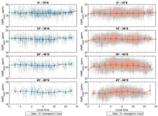
Figure 7.
Diurnal distribution of the water vapor volume mixing ratio in different latitude intervals in both hemispheres, presented separately. Light-blue (Northern Hemisphere) and orange (Southern Hemisphere) dots represent H2O VMR retrieved in individual observations. Vertical error bars show an individual retrieval uncertainty. Horizontal error bars illustrate the footprint diameter. Cross markers (Northern Hemisphere) and squares (Southern Hemisphere) correspond to the 1-h average. The average values are presented with STD.
4.3. Long-Term Trends
The SPICAV IR dataset comprises eight years of observations, representing the most extended continuous monitoring of water vapor in the deep Venus atmosphere to date. The obtained VMRs are analyzed to search for any possible long-term H2O variability. One limitation inherent in the dataset is its sparse spatial coverage. At a single orbit, i.e., in the course of one Earth day, only a small fraction (0.04–15%) of the night hemisphere is observed. Thus, temporal variability may be mixed with the potential spatial distribution of H2O.
The long-term evolution of H2O was examined in 15° latitude bins across both hemispheres. Figure 8 presents the individual retrievals in latitude bins over the course of the Venus Express mission from 2006 to 2014. To minimize experimental uncertainty when assessing long-term trends, and to improve the spatial coverage by accumulating footprints, the data was binned by 90 Earth days. The dataset revealed no apparent long-term trend.
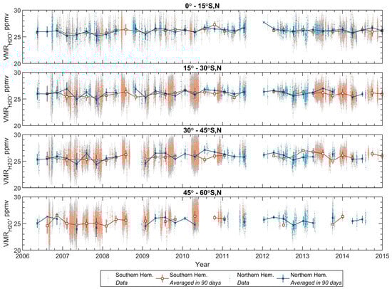
Figure 8.
Temporal distribution of the water vapor volume mixing ratio from 2006 to 2015 in different latitude intervals in both hemispheres. Light-blue (Northern Hemisphere) and orange (Southern Hemisphere) dots represent H2O VMR retrieved from individual observations in the Northern and Southern Hemispheres, respectively. Vertical error bars show individual retrieval uncertainty. Cross markers (Northern Hemisphere) and squares (Southern Hemisphere) correspond to the 90-day average. The average values are presented with STD.
5. Discussion
5.1. Water Vapor Spectroscopy Prospects
We investigated the impact of different spectroscopic model parameters on the shape of the spectrum in 1.1 and 1.18 μm transparency windows. Observed by SPICAV IR from space, this spectrum is free from the telluric water vapor absorption and acquired with the highest spectral resolution of all space instruments observing Venus. We can therefore examine the effect of the H2O line profile correction in detail. For these windows, different approximations of the sub-Lorentzian CO2 line profile have been considered using the “High-T” database [14]. In our work, we use an updated CO2 spectral line dataset incorporated in HITEMP containing ~50 times more spectral lines [44]. The CO2 continuum coefficient was recomputed using this database and two different CO2 line profiles (Table 2). The measured spectrum in the 1.1µm window was accurately (within the experimental uncertainties) represented by the synthetic model, which is achieved by adjusting line intensities and incorporating new lines of HITEMP [44]. Still, a satisfactory description of the 1.18 μm transparency-window spectrum was not achieved for either CO2 line shape approximations.
Prior studies have indicated the insufficient absorption of H2O near 1.125 and 1.140 μm in the synthetic spectra [14]. The CO2 and H2O line profiles, used in Ref. [14], are adopted in Model 1 of this work. Model 2, using the same CO2 line shape approximation (see Figure 4), represents the 1.125–1.140 μm range better, suggesting an insufficiency of the Voigt profile for H2O absorption computation. Water vapor line shape correction has the largest effect on the result. It should be noted that, in this paper, the super-Lorentz profile [10,50], incorporated into Model 3, was applied to a much larger number of spectral lines than in Ref. [10]. Consequently, Model 3 likely overestimates the water vapor absorption in combination with the BT2 line list [45].
The MT_CKD H2O model (Model 2) [49] and the super-Lorentz profile of Refs. [10,50] (Model 3) describe the H2O line wings as broadened by air. Ref. [60] compared the H2O line broadening by CO2 [61] with a predicted by the MT_CKD model in the range of 100–1500 cm−1 to find a stronger absorption. Their correction was obtained for temperatures of 296–366 K, corresponding to Venus’ cloud altitudes, and no temperature dependency was concluded. Our numerical experiment using the findings of [61] showed a greater H2O absorption than the MT_CKD model at 48–56 km for the 1.1 and 1.18 μm transparency windows. However, the MT_CKD model, which takes into account the change in temperature, results in a greater H2O absorption at 10–16 km than Ref. [61]. Given these ambiguities, we have not applied the H2O line profile correction recommended in [60,61] in the current study, underscoring the importance of further laboratory characterization of the H2O absorption in the spectral range of the Venus’ atmosphere transparency windows under relevant pressure and temperature.
5.2. Comparison with Previous Observations of H2O
The water vapor volume mixing ratios retrieved from the 1.1 and 1.18 μm transparency windows, using Model 1 and 2, to compute the H2O absorption are in good agreement with the heritage ground-based observations [10] revisited in Ref [12] using the high-temperature BT2 H2O line list, more recent observations [17] and a previous partial analysis of the SPICAV IR dataset [16]. Our mean H2O VMRs ranging, from 26.9 ± 1.0 to 27.7 ± 1.2 ppmv, are slightly below the 30+ 10−5 ppmv value obtained from early SPICAV analysis [14] and the 31+9−6 ppmv value from the 1.18-µm window telescope observations [15], yet they fall within the error bars of these experiments. Retrieval with Model 3 results in slightly lower VMRs (from 23.6 ± 1.0 to 24.0 ± 1.0 ppmv, Table 3) than previously obtained, suggesting again that Model 3 overestimates the H2O absorption.
Analyzing the complete SPICAV IR dataset, we conclude that the VMR error due to poorly constrained surface emissivity is below 0.6 ppmv. In Ref. [16], 20 orbits observed above Maxwell Montes were analyzed to retrieve a water vapor abundance of 25.7+1.4−1.2 for an emissivity of 0.95 and 29.4+1.6−1.4 for ε = 0.6. Their H2O VMR for ε = 0.95 is consistent, though a little lower than 27.1 ± 1.1 ppmv obtained for the complete SPICAV IR dataset. Their H2O VMR for ε = 0.6 is higher than 27.7 ± 1.2 ppmv obtained for ε = 0.4 in the current study. In Ref. [16], the value of the CO2 continuum coefficient has been modified along with the emissivity: α = 0.42 × 10⁻⁹ cm−1amagat−2 for ε = 0.95 and α = 0.66 × 10⁻⁹ cm−1amagat−2 for ε = 0.6 [16]. This study implements an alternative approach—freezing the continuum coefficient to its laboratory measurement [55]—to study the influence of other parameters. Nevertheless, the CO2 continuum is another factor potentially affecting the water vapor mixing ratio retrievals.
Observations of water vapor in higher atmospheric layers below the clouds result in similar VMR values of 30 ± 7.5 [7], 30 ± 10 [9], 25 ± 5 [20], 33 ± 2 and 32 ± 2 in 2010 [17] at ~20 km (the 1.74 μm transparency window) and 30 ± 6 [7], 30 +15−10 [9], 26 ± 4 [22], 31 ± 2 [23], (22–35) ± 4 [24], 34 ± 2 and 33 ± 3 (2010) [17], 32.0 ± 1.3 ppmv [26], 27 ± 3.5 [27] at ~35 km (the 2.3 μm transparency window), well matching our results at 10–16 km. Therefore, there is strong evidence that the vertical distribution of water vapor is uniform below the clouds. Venus’ atmosphere models also reproduce a uniform H2O mixing ratio ≤ 30 km because no source or sink is expected [62,63].
The SPICAV IR dataset covered almost the whole latitude range. Galileo spacecraft’s Near-Infrared Mapping Spectrometer showed the mean VMR of 30 ± 15 ppmv and the absence of horizontal variations exceeding 20% over a wide latitude range from 40° S to 50° N [8]. The H2O abundance at ~35 km did not demonstrate any variations within the latitude range of 60° S–60° N, which was defined by the spatial coverage of the VIRTIS-H dataset [27]. Both results are consistent with our nearly uniform latitude distribution of zonal mean from 60° S to 75° N. A possible 10% decrease in H2O VMR (from 33.0 ± 1.0 ppmv near the equator to 30.0 ± 2.5 ppmv at polar latitudes (>60° S)) in the Southern Hemisphere was suggested from the VIRTIS-M dataset analysis [26]. However, the result was interpreted with caution due to the analysis and experimental uncertainties estimated to be 30–47%, with higher errors obtained at high latitudes. The SPICAV IR dataset, for the first time, allowed us to address the H2O VMR at 10–16 km in polar latitudes, over 70°, of both hemispheres. The zonal mean VMR decreases by 2 ppmv above 60° S and at 75–85° N. Spectra obtained at these latitudes are characterized by an increased noise level. A two-dimensional circulation model of Venus’ atmosphere does not predict any latitude variations of the water vapor at 10–16 km [63]. The Venus Planetary Climate Model (Venus PCM), a three-dimensional general circulation model, demonstrates the influence of the Hadley cell circulation to water vapor at ~35 km [62], which is about 20 km higher than the altitudes, observed by SPICAV. The simulated mixing ratio at low and mid-latitudes is close to 30 ppmv and decreases to 27 ppmv at high latitudes at 35 km [62], resembling the pattern observed by SPICAV.
Prior to the Venus Express mission, only a few measurements of water vapor content in the lower atmosphere of Venus were obtained (Table 1). During the mission lifetime, a ground-based campaign run in 2009 and 2010 [17] demonstrated no significant temporal changes in water vapor content (see Table 1). An analysis of VIRTIS-H observations of the 2.3 μm transparency window in 2006–2011 also did not infer any long-term variability in the H2O VMR at ~35 km [27]. The water vapor bulk in the lower atmosphere of Venus sources the cloud layer and the mesosphere (>60 km) [62,64]. According to SPICAV IR day-side data, no temporal trend of water vapor at altitudes of 60–62 km was noticed [65]. A stable water vapor abundance is also confirmed by a ground-based observation campaign dedicated to HDO, as a proxy for H2O, at an altitude of 62 km in 2012–2015 [66]. Interestingly, observations carried out later, from 2016 to 2022, revealed a significant reduction in the water vapor content at these altitudes [66]. The SPICAV IR dataset demonstrates the stability of H2O in the lower atmosphere in 2006–2014. Further observations in the transparency windows will contribute to a more comprehensive understanding of the link between the lower and upper atmospheric layers.
The enhancement or depletion of water vapor abundance in the short term may be a consequence of the volcanic activity [4]. “Hot spots” [67,68] and landscape evolution [69,70] associated with the recent volcanism were found on Venus’ surface. A theoretical study of a potential water vapor plume was conducted assuming a “mid-sized” terrestrial eruption [4]. The maximal observable enhancement simulated near the volcanic source is about 0.8 ppmv at ~13 km [4]. Such a value is comparable but still below the estimated mean uncertainty ~1 ppmv of the SPICAV IR individual measurements. Strong deviations from the average mixing ratio of H2O that were not defined by experimental uncertainties have not been found in the retrieved values. A potential extension of this research would be to use averaged SPICAV observations with reduced experimental uncertainty, pronouncing the minor changes in water vapor.
6. Conclusions
We have analyzed the complete set of nadir observations of the Venus night side by the SPICAV IR spectrometer on board the Venus Express mission in 2006–2014. The dataset contains about 27000 spectra of Venus thermal emission in the 1.1 and 1.18 μm atmospheric transparency windows. In this spectral range, thermal emission originates from 0–15 km. The spectra are fitted by a radiative transfer model with multiple scattering and allow us to retrieve the H2O volume mixing ratio in the lower atmosphere of Venus at 10–16 km.
We compare, for the first time, different approaches to describe the water vapor absorption at high pressures and study their influence on the retrieved VMRs. When the Voigt profile is applied, the absorption is underestimated at 1.125 and 1.140 μm. Two H2O line shape approximations that introduce greater absorption in the far wings provide an optimal fit of the 1.1 and 1.18 μm transparency windows: the MT_CKD water vapor continuum model [49] and the super-Lorentzian line profile by Refs. [10,50]. Depending on the approach to calculate the H2O absorption, the global average of the volume mixing ratio is 27.1 ± 1.1 ppmv for the Voigt profile, 26.9 ± 1.0 ppmv for the MT_CKD H2O model and 23.6 ± 1.0 ppmv for the super-Lorentzian line profile. The absorption line model introduces higher uncertainty in the retrieved H2O VMR than the unknown surface emissivity. A surface emissivity of 0.4 results in average H2O VMRs of 27.7 ± 1.2 ppmv, 27.0 ± 1.1 ppmv and 24.0 ± 1.0 ppmv, respectively. The obtained average values are consistent with recent studies of water vapor below the cloud layer, indicating an H2O mixing ratio below 30 ppmv [14,16,17,27].
The SPICAV IR dataset covers the latitudes up to 84° in both hemispheres. The water vapor content at polar latitudes over 70° was studied for the first time at 10–16 km. The retrieved H2O spatial distribution is rather uniform in the lower atmosphere of Venus. The zonal mean of the water vapor VMR does not show significant variation across the range of 60° S–75° N. A slight decrease in H2O of 2 ppmv was observed at higher latitudes. However, observations at these latitudes are characterized by increased experimental uncertainties. A correlation between the topography and the retrieved water vapor abundance has not been detected. Moreover, the standard deviation of the H2O VMR in bins of 10° latitude and 10° longitude shows values of 0.8–1 ppmv, which are in correspondence with the STD for the entire dataset. There is no long-term trend and no local time dependence of water vapor in the lower atmosphere over 8 years.
Supplementary Materials
The following are available online at https://www.mdpi.com/article/10.3390/atmos16060726/s1, Figures S1.1–S1.3: Examples of analyzed spectra of 1.1 and 1.18 μm transparency windows fitted by the radiative transfer model assuming different surface emissivity; Figure S2: Distribution of H2O mixing ratio retrieved for different model parameters; Figure S3: Longitude distribution of the water vapor volume mixing ratio.
Author Contributions
Conceptualization, D.E. and A.F.; methodology, D.E., A.F., N.I. and J.-L.B.; software, D.E.; validation, D.E.; investigation, D.E.; resources, O.K.; data curation, D.E.; writing—original draft preparation, D.E.; writing—review and editing, D.E., A.F., N.I., O.K., F.M., J.-L.B.; visualization, D.E.; supervision, A.F. and F.M.; project administration, O.K. and F.M.; funding acquisition, D.E. All authors have read and agreed to the published version of the manuscript.
Funding
This work was financially supported by the Russian Science Foundation grant № 23-72-01064.
Institutional Review Board Statement
Not applicable.
Informed Consent Statement
Not applicable.
Data Availability Statement
The calibrated data and the observational geometry of the SPICAV IR experiment can be obtained from the ESA’s Planetary Science Archive (PSA): https://archives.esac.esa.int/psa/ (accessed on 14 June 2025).
Conflicts of Interest
The authors declare no conflicts of interest.
Abbreviations
The following abbreviations are used in this manuscript:
| IR, NIR | Infrared, Near-infrared |
| SPICAV | SPectroscopy for the Investigation of the Characteristics of the Atmosphere of Venus |
| VEx | Venus Express |
| AOTF | Acousto-optical tunable filter |
| VIRA | Venus International Reference Atmosphere |
| FOV | Field of view |
| VMR | Volume mixing ratio |
| STD | Standard deviation |
References
- Donahue, T.M.; Hoffman, J.H.; Hodges, R.R.; Watson, A.J. Venus Was Wet: A Measurement of the Ratio of Deuterium to Hydrogen. Science 1982, 216, 630–633. [Google Scholar] [CrossRef] [PubMed]
- Fedorova, A.; Korablev, O.; Vandaele, A.-C.; Bertaux, J.-L.; Belyaev, D.; Mahieux, A.; Neefs, E.; Wilquet, W.V.; Drummond, R.; Montmessin, F.; et al. HDO and H2O Vertical Distributions and Isotopic Ratio in the Venus Mesosphere by Solar Occultation at Infrared Spectrometer on Board Venus Express. J. Geophys. Res. 2008, 113. [Google Scholar] [CrossRef]
- Gérard, J.-C.; Bougher, S.W.; López-Valverde, M.A.; Pätzold, M.; Drossart, P.; Piccioni, G. Aeronomy of the Venus Upper Atmosphere. Space Sci. Rev. 2017, 212, 1617–1683. [Google Scholar] [CrossRef]
- Wilson, C.F.; Marcq, E.; Gillmann, C.; Widemann, T.; Korablev, O.; Mueller, N.T.; Lefèvre, M.; Rimmer, P.B.; Robert, S.; Zolotov, M.Y. Possible Effects of Volcanic Eruptions on the Modern Atmosphere of Venus. Space Sci. Rev. 2024, 220, 31. [Google Scholar] [CrossRef]
- Bullock, M.; Grinspoon, D. The Recent Evolution of Climate on Venus. Icarus 2001, 150, 19–37. [Google Scholar] [CrossRef]
- Allen, D.A.; Crawford, J.W. Cloud Structure on the Dark Side of Venus. Nature 1984, 307, 222–224. [Google Scholar] [CrossRef]
- Pollack, J.B.; Dalton, J.B.; Grinspoon, D.; Wattson, R.B.; Freedman, R.; Crisp, D.; Allen, D.A.; Bezard, B.; DeBergh, C.; Giver, L.P.; et al. Near-Infrared Light from Venus’ Nightside: A Spectroscopic Analysis. Icarus 1993, 103, 1–42. [Google Scholar] [CrossRef]
- Drossart, P.; Bézard, B.; Encrenaz, T.; Lellouch, E.; Roos, M.; Taylor, F.W.; Collard, A.D.; Calcutt, S.B.; Pollack, J.; Grinspoon, D.H.; et al. Search for Spatial Variations of the H2OAbundance in the Lower Atmosphere of Venus from NIMS-Galileo. Planet. Space Sci. 1993, 41, 495–504. [Google Scholar] [CrossRef]
- de Bergh, C.; Bézard, B.; Crisp, D.; Maillard, J.P.; Owen, T.; Pollack, J.; Grinspoon, D. Water in the Deep Atmosphere of Venus from High-Resolution Spectra of the Night Side. Adv. Space Res. 1995, 15, 79–88. [Google Scholar] [CrossRef]
- Meadows, V.S.; Crisp, D. Ground-Based near-Infrared Observations of the Venus Nightside: The Thermal Structure and Water Abundance near the Surface. J. Geophys. Res. Planets 1996, 101, 4595–4622. [Google Scholar] [CrossRef]
- Bézard, B.; Tsang, C.C.C.; Carlson, R.W.; Piccioni, G.; Marcq, E.; Drossart, P. Water Vapor Abundance near the Surface of Venus from Venus Express/VIRTIS Observations. J. Geophys. Res. Planets 2009, 114. [Google Scholar] [CrossRef]
- Bailey, J. A Comparison of Water Vapor Line Parameters for Modeling the Venus Deep Atmosphere. Icarus 2009, 201, 444–453. [Google Scholar] [CrossRef]
- Haus, R.; Arnold, G. Radiative Transfer in the Atmosphere of Venus and Application to Surface Emissivity Retrieval from VIRTIS/VEX Measurements. Planet. Space Sci. 2010, 58, 1578–1598. [Google Scholar] [CrossRef]
- Bézard, B.; Fedorova, A.; Bertaux, J.-L.; Rodin, A.; Korablev, O. The 1.10- and 1.18-Μm Nightside Windows of Venus Observed by SPICAV-IR Aboard Venus Express. Icarus 2011, 216, 173–183. [Google Scholar] [CrossRef]
- Chamberlain, S.; Bailey, J.; Crisp, D.; Meadows, V. Ground-Based near-Infrared Observations of Water Vapor in the Venus Troposphere. Icarus 2013, 222, 364–378. [Google Scholar] [CrossRef]
- Fedorova, A.; Bézard, B.; Bertaux, J.-L.; Korablev, O.; Wilson, C. The CO2 Continuum Absorption in the 1.10- and 1.18-Μm Windows on Venus from Maxwell Montes Transits by SPICAV IR Onboard Venus Express. Planet. Space Sci. 2015, 113–114, 66–77. [Google Scholar] [CrossRef]
- Arney, G.; Meadows, V.; Crisp, D.; Schmidt, S.J.; Bailey, J.; Robinson, T. Spatially Resolved Measurements of H2O, HCl, CO, OCS, SO2, Cloud Opacity, and Acid Concentration in the Venus near-Infrared Spectral Windows. J. Geophys. Res. Planets 2014, 119, 1860–1891. [Google Scholar] [CrossRef]
- Carlson, R.W.; Baines, K.H.; Encrenaz, T.; Taylor, F.W.; Drossart, P.; Kamp, L.W.; Pollack, J.B.; Lellouch, E.; Collard, A.D.; Calcutt, S.B.; et al. Galileo Infrared Imaging Spectroscopy Measurements at Venus. Science 1991, 253, 1541–1548. [Google Scholar] [CrossRef]
- Bezard, B.; de Bergh, C.; Crisp, D.; Maillard, J.-P. The Deep Atmosphere of Venus Revealed by High-Resolution Nightside Spectra. Nature 1990, 345, 508–511. [Google Scholar] [CrossRef]
- Iwagami, N.; Ohtsuki, S.; Tokuda, K.; Ohira, N.; Kasaba, Y.; Imamura, T.; Sagawa, H.; Hashimoto, G.L.; Takeuchi, S.; Ueno, M.; et al. Hemispheric Distributions of HCl above and below the Venus’ Clouds by Ground-Based 1.7 Μm Spectroscopy. Planet. Space Sci. 2008, 56, 1424–1434. [Google Scholar] [CrossRef]
- Bell, J.F.; Crisp, D.; Lucey, P.G.; Ozoroski, T.A.; Sinton, W.M.; Willis, S.C.; Campbell, B.A. Spectroscopic Observations of Bright and Dark Emission Features on the Night Side of Venus. Science 1991, 252, 1293–1296. [Google Scholar] [CrossRef] [PubMed]
- Marcq, E.; Encrenaz, T.; Bézard, B.; Birlan, M. Remote Sensing of Venus’ Lower Atmosphere from Ground-Based IR Spectroscopy: Latitudinal and Vertical Distribution of Minor Species. Planet. Space Sci. 2006, 54, 1360–1370. [Google Scholar] [CrossRef]
- Marcq, E.; Bézard, B.; Drossart, P.; Piccioni, G.; Reess, J.M.; Henry, F. A Latitudinal Survey of CO, OCS, H2O, and SO2 in the Lower Atmosphere of Venus: Spectroscopic Studies Using VIRTIS-H. J. Geophys. Res. Planets 2008, 113. [Google Scholar] [CrossRef]
- Tsang, C.C.C.; Wilson, C.F.; Barstow, J.K.; Irwin, P.G.J.; Taylor, F.W.; McGouldrick, K.; Piccioni, G.; Drossart, P.; Svedhem, H. Correlations between Cloud Thickness and Sub-cloud Water Abundance on Venus. Geophys. Res. Lett. 2010, 37. [Google Scholar] [CrossRef]
- Barstow, J.K.; Tsang, C.C.C.; Wilson, C.F.; Irwin, P.G.J.; Taylor, F.W.; McGouldrick, K.; Drossart, P.; Piccioni, G.; Tellmann, S. Models of the Global Cloud Structure on Venus Derived from Venus Express Observations. Icarus 2012, 217, 542–560. [Google Scholar] [CrossRef]
- Haus, R.; Kappel, D.; Arnold, G. Lower Atmosphere Minor Gas Abundances as Retrieved from Venus Express VIRTIS-M-IR Data at 2.3 µm. Planet. Space Sci. 2015, 105, 159–174. [Google Scholar] [CrossRef]
- Marcq, E.; Bézard, B.; Reess, J.-M.; Henry, F.; Érard, S.; Robert, S.; Montmessin, F.; Lefèvre, F.; Lefèvre, M.; Stolzenbach, A.; et al. Minor Species in Venus’ Night Side Troposphere as Observed by VIRTIS-H/Venus Express. Icarus 2023, 405, 115714. [Google Scholar] [CrossRef]
- Ignatiev, N.I.; Moroz, V.I.; Moshkin, B.E.; Ekonomov, A.P.; Gnedykh, V.I.; Grigoriev, A.V.; Khatuntsev, I.V. Water Vapor in the Lower Atmosphere of Venus: A New Analysis of Optical Spectra Measured by Entry Probes. Planet. Space Sci. 1997, 45, 427–438. [Google Scholar] [CrossRef]
- Korablev, O.; Fedorova, A.; Bertaux, J.-L.; Stepanov, A.V.; Kiselev, A.; Kalinnikov, Y.K.; Titov, A.Y.; Montmessin, F.; Dubois, J.P.; Villard, E.; et al. SPICAV IR Acousto-Optic Spectrometer Experiment on Venus Express. Planet. Space Sci. 2012, 65, 38–57. [Google Scholar] [CrossRef]
- Evdokimova, D.; Fedorova, A.; Ignatiev, N.; Zharikova, M.; Korablev, O.; Montmessin, F.; Bertaux, J.-L. Cloud opacity variations from nighttime observations in Venus transparency windows. Atmosphere 2025, 16, 572. [Google Scholar] [CrossRef]
- Stamnes, K.; Tsay, S.-C.; Wiscombe, W.; Jayaweera, K. Numerically Stable Algorithm for Discrete-Ordinate-Method Radiative Transfer in Multiple Scattering and Emitting Layered Media. Appl. Opt. 1988, 27, 2502. [Google Scholar] [CrossRef] [PubMed]
- Lin, Z.; Stamnes, S.; Jin, Z.; Laszlo, I.; Tsay, S.-C.; Wiscombe, W.J.; Stamnes, K. Improved Discrete Ordinate Solutions in the Presence of an Anisotropically Reflecting Lower Boundary: Upgrades of the DISORT Computational Tool. J. Quant. Spectrosc. Radiat. Transf. 2015, 157, 119–134. [Google Scholar] [CrossRef]
- Seiff, A.; Schofield, J.T.; Kliore, A.J.; Taylor, F.W.; Limaye, S.S.; Revercomb, H.E.; Sromovsky, L.A.; Kerzhanovich, V.V.; Moroz, V.I.; Marov, M.Y. Models of the Structure of the Atmosphere of Venus from the Surface to 100 Kilometers Altitude. Adv. Space Res. 1985, 5, 3–58. [Google Scholar] [CrossRef]
- Saunders, R.S.; Spear, A.J.; Allin, P.C.; Austin, R.S.; Berman, A.L.; Chandlee, R.C.; Clark, J.; Decharon, A.V.; De Jong, E.M.; Griffith, D.G.; et al. Magellan Mission Summary. J. Geophys. Res. Planets 1992, 97, 13067–13090. [Google Scholar] [CrossRef]
- Ford, P.G.; Pettengill, G.H. Venus Topography and Kilometer-scale Slopes. J. Geophys. Res. Planets 1992, 97, 13103–13114. [Google Scholar] [CrossRef]
- Haus, R.; Kappel, D.; Tellmann, S.; Arnold, G.; Piccioni, G.; Drossart, P.; Häusler, B. Radiative Energy Balance of Venus Based on Improved Models of the Middle and Lower Atmosphere. Icarus 2016, 272, 178–205. [Google Scholar] [CrossRef]
- Mishchenko, M.I.; Travis, L.D.; Lacis, A.A. Scattering, Absorption, and Emission of Light by Small Particles; Cambridge University Press: Cambridge, UK, 2002. [Google Scholar]
- Hashimoto, G.L.; Roos-Serote, M.; Sugita, S.; Gilmore, M.S.; Kamp, L.W.; Carlson, R.W.; Baines, K.H. Felsic Highland Crust on Venus Suggested by Galileo Near-Infrared Mapping Spectrometer Data. J. Geophys. Res. Planets 2008, 113. [Google Scholar] [CrossRef]
- Kappel, D.; Haus, R.; Arnold, G. Error Analysis for Retrieval of Venus’ IR Surface Emissivity from VIR-TIS/VEX Measurements. Planet. Space Sci. 2015, 113–114, 49–65. [Google Scholar] [CrossRef]
- Gilmore, M.; Treiman, A.; Helbert, J.; Smrekar, S. Venus Surface Composition Constrained by Observation and Experiment. Space Sci. Rev. 2017, 212, 1511–1540. [Google Scholar] [CrossRef]
- De Bergh, C.; Bézard, B.; Owen, T.; Crisp, D.; Maillard, J.-P.; Lutz, B.L. Deuterium on Venus: Observations From Earth. Science 1991, 251, 547–549. [Google Scholar] [CrossRef]
- Luginin, M.; Fedorova, A.; Belyaev, D.; Montmessin, F.; Korablev, O.; Bertaux, J.-L. Scale Heights and Detached Haze Layers in the Mesosphere of Venus from SPICAV IR Data. Icarus 2018, 311, 87–104. [Google Scholar] [CrossRef]
- Sneep, M.; Ubachs, W. Direct Measurement of the Rayleigh Scattering Cross Section in Various Gases. J. Quant. Spectrosc. Radiat. Transf. 2005, 92, 293–310. [Google Scholar] [CrossRef]
- Hargreaves, R.J.; Gordon, I.E.; Huang, X.; Toon, G.C.; Rothman, L.S. Updating the Carbon Dioxide Line List in HITEMP. J. Quant. Spectrosc. Radiat. Transf. 2025, 333, 109324. [Google Scholar] [CrossRef]
- Barber, R.J.; Tennyson, J.; Harris, G.J.; Tolchenov, R.N. A High-Accuracy Computed Water Line List. Mon. Not. R. Astron. Soc. 2006, 368, 1087–1094. [Google Scholar] [CrossRef]
- Lavrentieva, N.N.; Voronin, B.A.; Fedorova, A.A. H216O Line List for the Study of Atmospheres of Venus and Mars. Opt. Spectrosc. 2015, 118, 11–18. [Google Scholar] [CrossRef]
- Voronin, B.A.; Tennyson, J.; Tolchenov, R.N.; Lugovskoy, A.A.; Yurchenko, S.N. A High Accuracy Computed Line List for the HDO Molecule. Mon. Not. R. Astron. Soc. 2010, 402, 492–496. [Google Scholar] [CrossRef]
- Lavrentieva, N.N.; Voronin, B.A.; Naumenko, O.V.; Bykov, A.D.; Fedorova, A.A. Linelist of HD16O for Study of Atmosphere of Terrestrial Planets (Earth, Venus and Mars). Icarus 2014, 236, 38–47. [Google Scholar] [CrossRef]
- Mlawer, E.J.; Cady-Pereira, K.E.; Mascio, J.; Gordon, I.E. The Inclusion of the MT_CKD Water Vapor Continuum Model in the HITRAN Molecular Spectroscopic Database. J. Quant. Spectrosc. Radiat. Transf. 2023, 306, 108645. [Google Scholar] [CrossRef]
- Clough, S.A.; Kneizys, F.X.; Davies, R.W. Line Shape and the Water Vapor Continuum. Atmos. Res. 1989, 23, 229–241. [Google Scholar] [CrossRef]
- Koroleva, A.O.; Kassi, S.; Mondelain, D.; Campargue, A. The Water Vapor Foreign Continuum in the 8100–8500 Cm−1 Spectral Range. J. Quant. Spectrosc. Radiat. Transf. 2023, 296, 108432. [Google Scholar] [CrossRef]
- Gordon, I.E.; Rothman, L.S.; Hargreaves, R.J.; Hashemi, R.; Karlovets, E.V.; Skinner, F.M.; Conway, E.K.; Hill, C.; Kochanov, R.V.; Tan, Y.; et al. The HITRAN2020 Molecular Spectroscopic Database. J. Quant. Spectrosc. Radiat. Transf. 2022, 277, 107949. [Google Scholar] [CrossRef]
- Fedorova, A.A.; Trokhimovsky, S.; Korablev, O.; Montmessin, F. Viking Observation of Water Vapor on Mars: Revision from up-to-Date Spectroscopy and Atmospheric Models. Icarus 2010, 208, 156–164. [Google Scholar] [CrossRef]
- Helbert, J.; Maturilli, A.; Dyar, M.D.; Alemanno, G. Deriving Iron Contents from Past and Future Venus Surface Spectra with New High-Temperature Laboratory Emissivity Data. Sci. Adv. 2021, 7, eaba9428. [Google Scholar] [CrossRef] [PubMed]
- Snels, M.; Stefani, S.; Piccioni, G.; Bèzard, B. Carbon Dioxide Absorption at High Densities in the 1.18 μm Nightside Transparency Window of Venus. J. Quant. Spectrosc. Radiat. Transf. 2014, 133, 464–471. [Google Scholar] [CrossRef]
- Palmer, K.F.; Williams, D. Optical Constants of Sulfuric Acid; Application to the Clouds of Venus? Appl. Opt. 1975, 14, 208–219. [Google Scholar] [CrossRef]
- Lagarias, J.C.; Reeds, J.A.; Wright, M.H.; Wright, P.E. Convergence Properties of the Nelder--Mead Simplex Method in Low Dimensions. SIAM J. Optim. 1998, 9, 112–147. [Google Scholar] [CrossRef]
- Tyler, G.L.; Ford, P.G.; Campbell, D.B.; Elachi, C.; Pettengill, G.H.; Simpson, R.A. Magellan: Electrical and Physical Properties of Venus’ Surface. Science 1991, 252, 265–270. [Google Scholar] [CrossRef]
- Ekonomov, A.P.; Golovin, Y.M.; Moshkin, B.E. Visible Radiation Observed near the Surface of Venus: Results and Their Interpretation. Icarus 1980, 41, 65–75. [Google Scholar] [CrossRef]
- Fakhardji, W.; Tran, H.; Pirali, O.; Hartmann, J.-M. The H2O–CO2 Continuum around 3.1, 5.2 and 8.0 μm: New Measurements and Validation of a Previously Proposed χ Factor. Icarus 2023, 389, 115217. [Google Scholar] [CrossRef]
- Tran, H.; Turbet, M.; Hanoufa, S.; Landsheere, X.; Chelin, P.; Ma, Q.; Hartmann, J.-M. The CO2–Broadened H2O Continuum in the 100–1500 Cm−1 Region: Measurements, Predictions and Empirical Model. J. Quant. Spectrosc. Radiat. Transf. 2019, 230, 75–80. [Google Scholar] [CrossRef]
- Stolzenbach, A.; Lefèvre, F.; Lebonnois, S.; Määttänen, A. Three-Dimensional Modeling of Venus Photochemistry and Clouds. Icarus 2023, 395, 115447. [Google Scholar] [CrossRef]
- Kuwayama, S.; Hashimoto, G.L. Meridional Distribution of CO, H2 O, and H2 SO4 in the Venus’ Atmosphere: A Two-Dimensional Model Incorporating Transport and Chemical Reaction. J. Geophys. Res. Planets 2025, 130, e2024JE008596. [Google Scholar] [CrossRef]
- Titov, D.V.; Ignatiev, N.I.; McGouldrick, K.; Wilquet, V.; Wilson, C.F. Clouds and Hazes of Venus. Space Sci. Rev. 2018, 214, 126. [Google Scholar] [CrossRef]
- Fedorova, A.; Marcq, E.; Luginin, M.; Korablev, O.; Bertaux, J.-L.; Montmessin, F. Variations of Water Vapor and Cloud Top Altitude in the Venus’ Mesosphere from SPICAV/VEx Observations. Icarus 2016, 275, 143–162. [Google Scholar] [CrossRef]
- Encrenaz, T.; Greathouse, T.K.; Giles, R.; Widemann, T.; Bézard, B.; Lefèvre, M.; Shao, W. HDO and SO2 Thermal Mapping on Venus: VI. Anomalous SO2 Behavior during Late 2021. Astron. Astrophys. 2023, 674, A199. [Google Scholar] [CrossRef]
- Smrekar, S.E.; Stofan, E.R.; Mueller, N.; Treiman, A.; Elkins-Tanton, L.; Helbert, J.; Piccioni, G.; Drossart, P. Recent Hotspot Volcanism on Venus from VIRTIS Emissivity Data. Science 2010, 328, 605–608. [Google Scholar] [CrossRef] [PubMed]
- Shalygin, E.V.; Markiewicz, W.J.; Basilevsky, A.T.; Titov, D.V.; Ignatiev, N.I.; Head, J.W. Active Volcanism on Venus in the Ganiki Chasma Rift Zone. Geophys. Res. Lett. 2015, 42, 4762–4769. [Google Scholar] [CrossRef]
- Herrick, R.R.; Hensley, S. Surface Changes Observed on a Venusian Volcano during the Magellan Mission. Science 2023, 379, 1205–1208. [Google Scholar] [CrossRef]
- Sulcanese, D.; Mitri, G.; Mastrogiuseppe, M. Evidence of Ongoing Volcanic Activity on Venus Revealed by Magellan Radar. Nat. Astron. 2024, 8, 973–982. [Google Scholar] [CrossRef]
Disclaimer/Publisher’s Note: The statements, opinions and data contained in all publications are solely those of the individual author(s) and contributor(s) and not of MDPI and/or the editor(s). MDPI and/or the editor(s) disclaim responsibility for any injury to people or property resulting from any ideas, methods, instructions or products referred to in the content. |
© 2025 by the authors. Licensee MDPI, Basel, Switzerland. This article is an open access article distributed under the terms and conditions of the Creative Commons Attribution (CC BY) license (https://creativecommons.org/licenses/by/4.0/).