Article

D- and F-Region Ionospheric Response to the Severe Geomagnetic Storm of April 2023

by
Arnab Sen
1,2,
Sujay Pal
3,*,
Bakul Das
4 and
Sushanta K. Mondal
1
1
Department of Physics, Sidho Kanho Birsha University, Purulia 723104, West Bengal, India
2
North East Regional Institute of Education, National Council of Educational Research and Training, Shillong 793103, Meghalaya, India
3
Department of Physics, Srikrishna College, Bagula 741502, West Bengal, India
4
Department of Physics, Cooch Behar Panchanan Barma University, Cooch Behar 736101, West Bengal, India
*
Author to whom correspondence should be addressed.
Atmosphere 2025, 16(6), 716; https://doi.org/10.3390/atmos16060716
Submission received: 13 May 2025 / Revised: 28 May 2025 / Accepted: 10 June 2025 / Published: 13 June 2025

Abstract

This study investigates the impact on the Earth’s ionosphere of a severe geomagnetic storm (Dst    212 nT) that began on 23 April 2023 at around 17:37 UT according to very low-frequency (VLF, 3–30 kHz) or low-frequency (LF, 30–300 kHz) radio signals and ionosonde data. We analyze VLF/LF signals received by SuperSID monitors located in mid-latitude (Europe) and low-latitude (South America, Colombia) areas across nine different propagation paths in the Northern Hemisphere. Mid-latitude regions exhibited a daytime amplitude perturbation, mostly an increase, by ∼3–5 dB during the storm period, with a subsequent recovery after 7–8 days post April 23. In contrast, signals received in low-latitude regions (UTP, Colombia) did not show significant variation during the storm-disturbed days. We also observe that the 3-hour average of foF2 data declined by up to 3 MHz on April 23 and April 24 at the European Digisonde stations. However, no significant variation in foF2 was observed at the low-latitude Digisonde stations in Brazil. Both the VLF and ionosonde data exhibited anomalies during the storm period in the European regions, confirming that both D- and F-region ionospheric perturbation was caused by the severe geomagnetic storm.

1. Introduction

A powerful Coronal Mass Ejection (CME), when entering the inter planetary space of the Earth, is referred to as an Interplanetary Coronal Mass Ejection (ICME). If an ICME contains a strong and sustained southward magnetic field ( B z < 0 for > 3 h), it can interact intensely with the Earth’s magnetosphere, triggering geomagnetic storms and space weather disruptions [1,2]. Geomagnetic storms thus occur when transient solar events such as CMEs and high-speed solar wind streams release energetic charged particles into the magnetosphere, driving currents and energy transfer processes that lead to a temporary decrease in the horizontal component of the geomagnetic field, followed by a recovery period [3,4]. The severity of geomagnetic storms can have a great impact on space and communication technologies. A moderate storm in February 2022 destroyed 38 of 49 Starlink SpaceX satellites a day after launch, when they were about to be lifted to a higher Earth orbit within the Earth’s magnetosphere [5].
Earth’s magnetosphere is a region of space surrounding the Earth, dominated by its magnetic field. This magnetic field traps and controls the motion of charged particles from solar wind, creating a protective shield against the harmful effects of solar and cosmic radiation. The solar wind compresses the Earth’s magnetic field, and hence, on the day side (the sun-facing side), the magnetosphere typically extends up to 10–11 R E (where R E is the Earth’s radius), and on the side facing away from the Sun (the night side), it may extend up to 60–100 R E [6,7]. When energetic particles precipitate into the ionosphere during a geomagnetic storm, they cause excess ionization, increasing the electron density and ionospheric conductivity [8]. Geomagnetic storms induce electric current in the Earth’s magnetosphere and ionosphere and increase auroral activity. The auroral electrojet expands toward mid-latitudes and precipitates particles in the mid-latitude ionosphere. High-latitude regions experience immediate effects from geomagnetic storms, while mid-latitude regions are more affected by post-storm effects, causing prolonged disturbances [9,10,11].
Ionospheric storms typically follow geomagnetic storms. When geomagnetic storms occur, they can alter the density and composition of the ionosphere, causing ionospheric storms. Ionospheric storms mainly cause disturbances in the F-layer ionosphere and have prolonged effects mainly over mid-latitudes [12]. Geomagnetic storms can lead to either positive or negative ionospheric storms depending on their impact on the ionosphere. Positive ionospheric storms occur when there is excess ionization, resulting in higher electron density due to the influx of energetic particles. Conversely, negative ionospheric storms arise from increased ionospheric heating and disturbances, which alter the ionosphere’s composition and dynamics, leading to reduced electron density, particularly in the F-layer [13]. Since atomic oxygen (O) is more easily ionized by solar radiation, it is a primary contributor to the ionospheric electron density, and the ratio of atomic oxygen to molecular nitrogen ( O / N 2 ) is a determinant factor of ionospheric storms [14]. During geomagnetic storms, enhanced ionization can sometimes increase the recombination rate, further decreasing the electron density in a negative ionospheric storm [13,15,16]. Variations in electron density can propagate through the ionosphere horizontally or vertically in a wave-like manner, known as Traveling Ionospheric Disturbances (TIDs). Large-scale TIDs (LSTIDs), with horizontal wavelengths > 1000 km, are typically generated in high latitudes and can travel to the equator at horizontal speeds greater than >250 m/s [17,18]. The periodic variation of the electron density along the TID propagation path can affect the reflection of high-frequency (HF, 3–30 MHz) waves from the upper ionosphere, which can be observed in ionosonde data. TIDs can alter the distribution of electron density and amplify the effects of a negative ionospheric storm.
The mid-latitude ionospheric trough (MIT) also plays a significant role in the variation of electron density in the mid-latitudes. The MIT is a region of low electron density that forms in the nighttime F-layer over mid-latitudes [19]. During geomagnetic storms, this trough deepens and moves equatorward, contributing to negative ionospheric storms [20]. Nayak et al. [21] reported that the equatorward shift of the MIT and chemical compositional changes in the mid-latitude region over Europe led to negative ionospheric storms during the super geomagnetic storm that began on 17 March 2015. Oikonomou et al. [22] investigated the geomagnetic storms of 7–8 September 2017 and attributed the formation of negative ionospheric storms over the mid-latitude European region to the equatorward shift of MIT. The geomagnetic storm that started on 23 April 2023 triggered by a powerful CME was one of the major storms in Solar Cycle 25. This geomagnetic storm is considered severe according to the National Oceanic and Atmospheric Administration (NOAA) Space Weather Scale (https://www.swpc.noaa.gov/noaa-scales-explanation (accessed on 13 May 2024)) since the K p index reached 8+ on April 23 and 24 (see Figure 1). The severe geomagnetic storm of April 2023 induced a negative ionospheric storm [2,23].
The ionosphere below 90 km reflects very low-frequency (VLF, 3–30 kHz) and low-frequency (LF, 30–300 kHz) signals, which travel within a waveguide formed by the Earth and the boundary of the lower ionosphere (60–90 km) [24]. The VLF/LF waves are continuously transmitted by ground-based transmitters, mostly used for submarine communication by the Navy. VLF signals exhibit regular diurnal and seasonal variations in signal amplitudes primarily due to the solar ionization of the lower ionosphere. Since VLF/LF wave propagation is sensitive to changes in the electrical conductivity of the lower ionospheric boundary, these waves are effectively utilized to probe various external ionospheric disturbances on different timescales, including solar flares [25,26,27], solar eclipses [28,29], gamma-ray bursts [30], geomagnetic activities [31,32,33], lightning-induced events [34,35], and sudden stratospheric warming (SSW) events [36,37], etc.
Geomagnetic storms mainly affect high-to-mid latitude regions, and unusual variations in VLF/LF signal amplitudes can be observed during storm periods [33]. Mondal et al. [11] studied the variations in VLF radio signals due to the super geomagnetic storm of 17 March 2015 along the propagation paths over the mid-latitude region. In the current paper we investigate the impact of a severe geomagnetic storm that commenced on 23 April 2023. We analyzed VLF/LF signals transmitted from six stations and received by Stanford SuperSID monitors at two locations in Europe and one in Colombia, across nine propagation paths during the pre- to post-storm period. We also compared the critical frequency of the F2 layer (foF2) of the ionosphere during this period to observe the upper ionospheric response to the geomagnetic storm. We chose the ionosonde receivers closest to the VLF receivers. We report a unique approach of simultaneously observing the D-region and F-region ionosphere during a severe geomagnetic storm and also broaden the spatial analysis. This research further examines the time delay in the responses of the different regions of the ionosphere to the geomagnetic storm.
In the next section, we give the details of the VLF/LF transmitters and receivers used in this study, along with the ionosonde receivers. We present our results in Section 3, and finally, in Section 4, we conclude the work discussing the results with possible explanations.

2. Data and Methodology

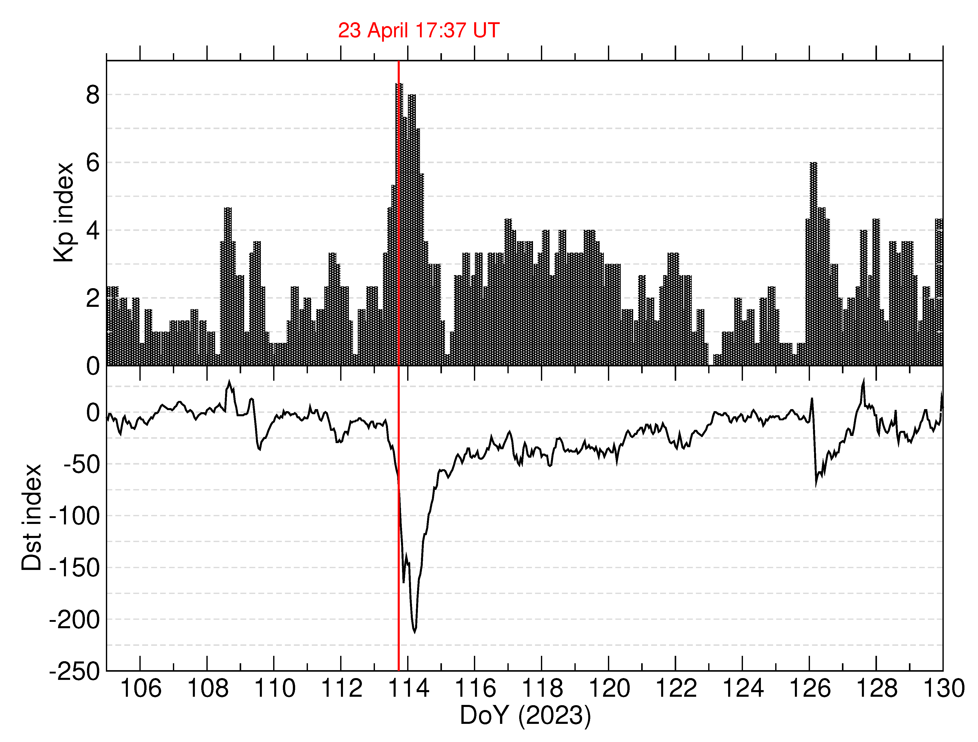
2.1. Geomagnetic Storm Indices
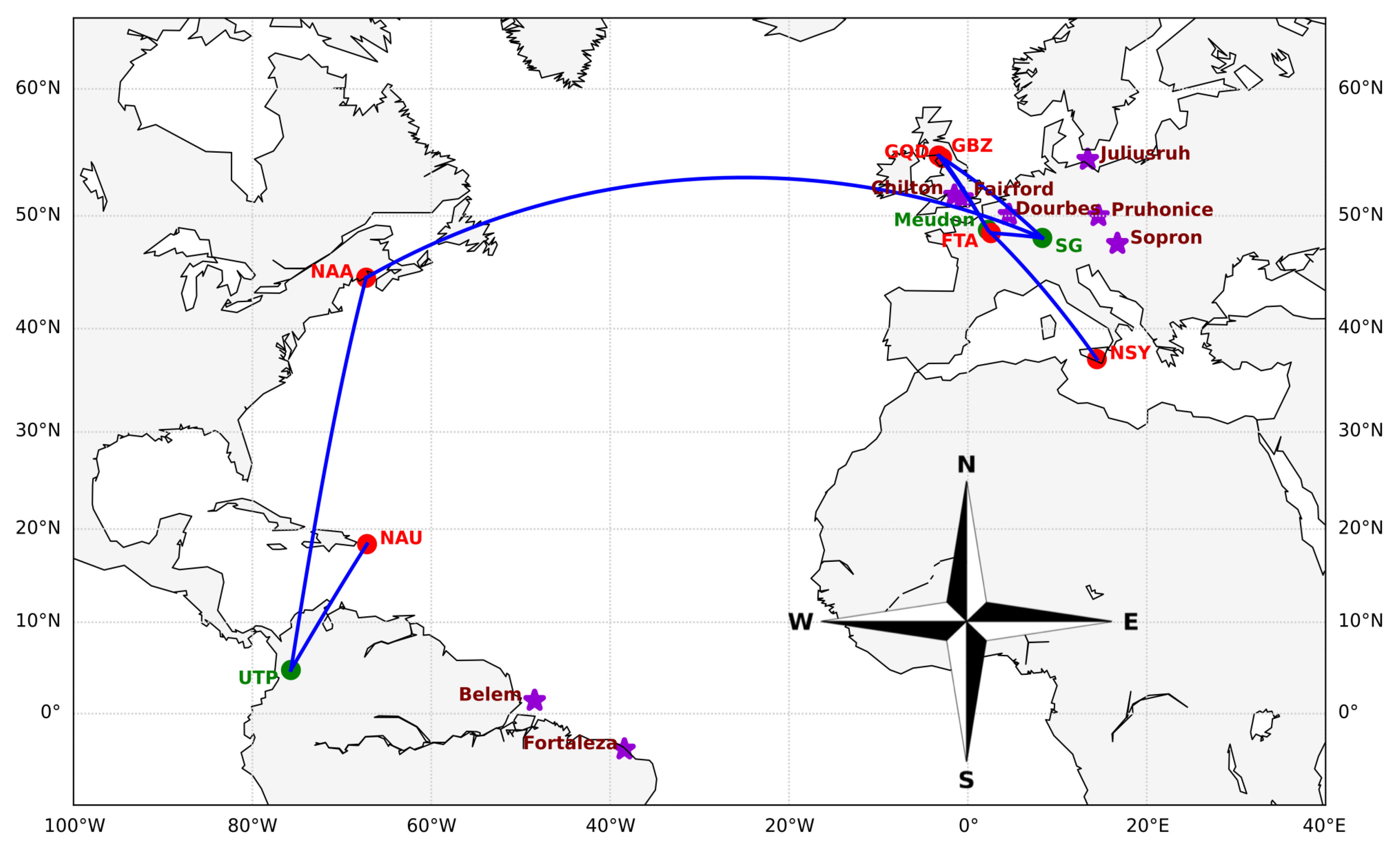
Geomagnetic storms enhance current systems in the Earth’s magnetosphere and ionosphere. The currents along the geomagnetic field lines, called field-aligned currents, couple the auroral ionosphere and drive auroral electrojets, causing significant disturbances in the geomagnetic field [38]. The K p index (Planetary K-index) quantifies disturbances in the horizontal component of the Earth’s magnetic field with an integer in the 0–9 range, with 1 being calm and 5 or more indicating a geomagnetic storm [39]. During geomagnetic storms, a strong ring current develops due to the trapped charged particles in the magnetosphere, primarily around the equatorial plane. The Dst index (Disturbance Storm Time index) is derived from measurements of the horizontal component of the Earth’s magnetic field, primarily influenced by the ring current [40]. The values of the K p and Dst indices signify the strength of geomagnetic storms. A geomagnetic storm consists of three phases—the initial, main, and recovery phases—each with variable time scales [1]. The initial phase lasts from a few minutes to several hours and is marked by an increase in Dst to positive values due to enhanced solar wind ram pressure. The main phase, lasting from about 30 min to several hours, begins when Dst starts decreasing, indicating the intensification of the ring current. Finally, during the recovery phase, which can extend from several hours to a week, Dst gradually returns to its pre-storm levels as the ring current dissipates [41].
The geomagnetic storm indices K p and Dst obtained from the World Data Center for Geomagnetism, Kyoto, Japan (https://wdc.kugi.kyoto-u.ac.jp (accessed on 7 December 2023)) are plotted in Figure 1 for the pre- to post-storm period (15 April–10 May 2023). The top panel of Figure 1 shows that the K p index started to increase above 6 on the evening of April 23 (Day of Year (DoY) 113), when the storm initiated, reaching 8+ on two occasions and remaining high during April 23 and 24. The Dst index in the bottom panel shows that Dst dropped below −100 nT on the evening of April 23 and further to about −212 nT, indicating a severe geomagnetic storm.

2.2. VLF/LF Data

We make use of the VLF data recorded by SuperSID receivers (SID stands for Sudden Ionospheric Disturbance) and maintained by the SuperSID program (http://sid.stanford.edu/database-browser/ (accessed on 6 June 2023)) of the Solar Center of Stanford University, Stanford, CA, USA. We analyze VLF signals at three sites: DE_St_Georgen, Germany ( 48.12 ° N, 8.33 ° E); SID_Meudon, France ( 48.81 ° N, 2.23 ° E); and UTP, Colombia ( 4.79 ° N, 75.69 ° W). The signals were transmitted from FTA (63.85 kHz), GBZ (19.58 kHz), GQD (22.1 kHz), NAA (24.0 kHz), NSY (45.9 kHz), and NAU (40.8 kHz) transmitters.
We consider nine different propagation paths: FTA to DE_St_Georgen, GBZ to DE_St_Georgen, GQD to DE_St_Georgen, NAA to DE_St_Georgen, GBZ to SID_Meudon, GQD to SID_Meudon, NSY to SID_Meudon, NAU to UTP, and NAA to UTP. The coordinates and locations of the transmitters and receivers for these propagation paths are presented in Table 1. We considered long paths as those extending over several thousand kilometers, particularly trans-oceanic paths where the signal propagates over vast ionospheric regions. The NAA-DE_St_Georgen path is the longest, with a great circle length of approximately 5500 km, and runs west-to-east. Another long path is NAA-UTP, which is about 4450 km long and runs north-to-west. The shortest path is FTA-DE_St_Georgen, with a length of approximately 440 km and a west-to-east direction. The local time offsets with respect to UT for the European locations are 1–2 h, whereas for the South American location (UTP, Colombia), it is UT–5 h. The diurnal variations of VLF signal amplitudes along a propagation path follow the local time of the receiver’s location. The VLF propagation paths cover mid-latitude and low-latitude regions where we studied the storm’s impact on the ionosphere. The corresponding Great Circle Paths (GCPs) are shown in Figure 2.

2.3. Ionosonde Data

To compare the changes in the lower ionosphere (probed by the VLF signals) with the upper ionosphere, we also study foF2 data during the geomagnetic storm of April 2023. We analyze foF2 data recorded by the Global Ionosphere Radio Observatory (GIRO) of Lowell Digisonde International, Lowell, MA, USA, which performs simultaneous measurements every 5 to 15 min at over 60 locations worldwide. We used the auto-scaled foF2 data from the Digisonde DPS-4D stations at eight locations, including six in Europe and two in South America.
The European locations are Dourbes, Belgium ( 50.1 ° N, 4.6 ° E); Juliusruh, Germany ( 54.6 ° N, 13.4 ° E); Pruhonice, Czech Republic ( 50 ° N, 14.6 ° E); Sopron, Hungary ( 47.63 ° N, 16.72 ° E); Fairford, England ( 51.7 ° N, 1.5 ° W); and Chilton, UK ( 51.5 ° N, 0.6 ° W). The South American locations are Belem, Brazil ( 1.43 ° N, 48.44 ° W), and Fortaleza, Brazil ( 3.9 ° S, 38.4 ° W). We chose the Digisonde stations in Europe located close to the SuperSID monitors whose VLF data we are studying. Similarly, the Digisonde stations in South America were chosen based on their proximity to VLF receiver UTP, Colombia, and the availability of foF2 data during the study period. The Digisonde stations are marked with violet star symbols in Figure 2, where the VLF/LF transmitters are indicated by red dots, the VLF/LF receivers by green dots, and the VLF/LF propagation paths are depicted by blue lines.

3. Results

3.1. Diurnal Variations of VLF/LF Signals

The impact of the geomagnetic storm on the ionosphere was studied by analyzing VLF data from the pre-storm to post-storm period along nine propagation paths, as detailed in Table 1. To compare the signal amplitude variations during the storm days, we analyze the SuperSID VLF/LF data from April 18 to May 5 (DoY 108 125 ) for all the paths corresponding to receivers located in Europe. The data for the paths associated with the UTP receiver were analyzed from April 18 to April 30 (DoY 108 120 ), as the SuperSID data at UTP, Colombia, were inconsistent during the period of May 1 5 . VLF data during the period of 18 22 April is considered normal day data or unperturbed data. Our selection of normal days or quiet days was based on short-term quiet conditions rather than long-term statistical analysis, since the objective is to determine the variations due to the sudden disturbance. In event-based studies such as geomagnetic storms, using a shorter reference period immediately preceding the event ensures that the background ionospheric state is comparable to the perturbed state. This minimizes potential influences from long-term seasonal or solar cycle variations. We create an average day profile from this normal day data for various receiver-transmitter sets and calculate the corresponding standard deviation ( σ ), which is the measure of quiet day dispersion. We compare the storm-affected data of 23 April onward with this unperturbed profile to understand the influence of the storm in the diurnal VLF signals in the subsequent days.
Figure 3 illustrates the time series of diurnal variations of VLF/LF signals received at DE_St_Georgen, Germany, from transmitters FTA (Figure 3a) and GBZ (Figure 3c). The time series plots are colored red, with the blue vertical line indicating the beginning of the storm on April 23. Green circles represent the daytime average values computed over a 2-hour interval (12–14 UT) around mid-day, connected by green dotted lines. The diurnal variations of VLF/LF signals from FTA and GBZ during the storm-disturbed days (April 23–28) are presented in Figure 3b and Figure 3d, respectively. The gray shading in all sub-figures of Figure 3 represents the average signal amplitude of pre-storm days or normal days (April 18–22) ± 2 σ . The average signal of the pre-storm days is indicated by a black dashed curve. From Figure 3b,d it can be clearly seen that on many occasions, post-storm signals deviate beyond the ± 2 σ level of the normal day profile. In the case of FTA, the daytime signal from 8 14 UT is attenuated, and minimum attenuation occurred on April 25. This is marked by a black arrow in Figure 3a. Significant deviation of the signal amplitude was also observed during sunrise and sunset on April 25. In the case of GBZ, VLF signals are more affected during the period of sunrise (4–6 UT) and sunset (18–20 UT). The maximum deviations were observed during the sunset of April 25 and sunrise of April 26. These are indicated by black arrows in Figure 3c. The nighttime signals along FTA–DE_St_Georgen path are noiser than the GBZ–DE_St_Georgen path (see Figure 3b,d). This could happen because FTA (63.85 kHz, LF) waves are more susceptible to absorption in the lower ionosphere (D-region) compared to GBZ (19.58 kHz, VLF) waves. LF signals experience greater attenuation due to ionospheric absorption, especially during night-time conditions, when recombination processes reduce free electron density. The fluctuating ionization levels in the nighttime lower ionosphere can introduce more variability in LF signals, making them appear noisier. VLF waves (GBZ, 19.58 kHz) propagate more efficiently in the Earth ionosphere waveguide with less attenuation and are generally more stable at night.
Figure 4a,c depict the time series plots (colored red) of diurnal variations of VLF signals from GQD ( 22.1 kHz) and NAA (24 kHz) transmitters, respectively. Both the signals were received at DE_St_Georgen, Germany. From Figure 2 it can be seen that NAA signals traverse a long trans-oceanic path, while GQD signals traverse a short path to DE_St_Georgen, Germany, similar to the GBZ–DE_St_Georgen path. The diurnal variations of VLF signals on storm-disturbed days are shown in Figure 4b,c. It is seen that in the mid-latitude long paths, the VLF signal gain drastically increases; in Figure 4c, one can notice that the the whole-day signals went up for several days in the post-storm period. The 2-hour mid-day signal average (indicated by green circles connected by green dotted lines) is well beyond the ± 2 σ level. The signals during the disturbed days along the NAA–DE_St_Georgen also significantly rose post-sunset (21–24 UT). The signal amplitudes at DE_St_Georgen, Germany increased by about ∼3–5 dB during daytime on April 26, and significant fluctuations were observed during sunrise and sunset (see Figure 4d). The peak variation of the signal amplitude along the NAA–DE_St_Georgen path is marked by a black arrow in Figure 4c. In the shorter GQD–DE_St_Georgen path, the variation is not so prominent in the daytime except the sunrise–sunset period. The short peak in the daytime signal of April 27 is due to a M1.88 solar flare with a peak around 11:14 UT. The VLF signals along the GBZ–DE_St_Georgen path was not affected during the M1.88-class solar flare. This can happen due to the changes in phase velocities and the signal attenuation coefficient due to solar flares. Some propagation paths may always show positive VLF amplitude response, some may show negative amplitude response, and some other propagation paths may show both positive and negative amplitude responses due to the solar flare with no response corresponding to a certain class of flare. This has been shown explicitly in Barman et al. [42], where they reported a null VLF amplitude response for a propagation path corresponding to a certain class of solar flare but positive and negative amplitude responses for all other classes of flares.
The variations of the VLF/LF signals from three transmitters, GBZ, GQD, and NSY, received at Meudon, France, are presented in Figure 5. All these propagation paths are short paths. The time series of diurnal variations in signal amplitude are plotted in Figure 5a,c,e. The diurnal variations of VLF/LF signal amplitudes on storm-disturbed days (April 23–28) are shown in Figure 5b,d,f. The signal amplitude variations along the GQD–Meudon and NSY–Meudon paths are more prominent, and daytime VLF amplitude increased by a maximum ∼3–5 dB during the post-storm days. Along the GBZ–Meudon path, an anomaly in the signal amplitudes was observed only during sunrise and sunset time. The peak variations are marked by black arrows in Figure 5c,e. The propagation paths for GBZ–Meudon (19.58 kHz) and GQD–Meudon (22.1 kHz) are similar, as both transmitters are located in the UK and are received at Meudon, France. A clear difference in signal behavior between these two near-identical paths has been observed. This may happen due to the difference in the transmission frequency and transmitting power of each transmitting antenna. Higher-frequency VLF waves generally experience lower reflection heights and higher attenuation in the D-region, which can lead to differences in received signal strength and stability. Even a small difference in frequency can lead to slightly different modal interference patterns along the propagation path. The transmitting power of each transmitting antenna also can contribute to the signal variations received at a particular receiving location. Though these two paths may look identical position-wise, signal reception along these paths may vary significantly.
In Figure 6, the time series plot of VLF/LF signals from NAU and NAA transmitters received at UTP, Colombia, is presented for 18–30 April, 2023. Green circles in the time-series plots (Figure 6a,c) represent the daytime average values computed over a 2-hour interval (18–20 UT) around mid-day, connected by green dotted lines. The data from May 1 to May 5 were either unavailable or noisy. The diurnal variations of the signal amplitude during the storm days (April 23–28) are shown in Figure 6b,d. No significant variation in the VLF/LF signal amplitude was observed at the UTP, Colombia, site. Because UTP is a low-latitude receiving station, neither the long path propagation (NAA-UTP) nor the short path propagation (NAU-UTP) was affected by the severe storm.
Figure 7 presents the variation in daytime amplitude deviations across all nine VLF/LF propagation paths during the period from April 8 to May 5 (DoY 108–124). The daytime amplitude deviation was calculated by subtracting the mean signal amplitude of the pre-storm days (April 18–22) from the average diurnal amplitude of each day during the period of the study. The black bars represent the daytime amplitude deviation computed over a 2-hour interval (12–14 UT for the European sectors and 18–20 UT for UTP, Colombia). The red curve overlaid on each plot shows the variation of the Dst index throughout the study period. The FTA–St. Georgen path exhibited a negative deviation exceeding ∼5 dB on April 25 (DoY 115), two days after the beginning of the geomagnetic storm. No significant deviation was observed along the GBZ–St. Georgen and GQD–St. Georgen paths. The NAA–St. Georgen path showed a moderate positive variation of up to 3 dB on April 26 and 27 (DoY 116 and 117). Among the paths with a receiver at Meudon, the GBZ–Meudon path displayed no significant variation, while the GQD–Meudon path exhibited a deviation of approximately 4 dB on April 26 (DoY 116). The NSY–Meudon path showed a variation exceeding 3 dB on the same day. There was no significant variation of average daytime signals received at UTP, Colombia, along both the NAU–UTP and NAA–UTP paths.

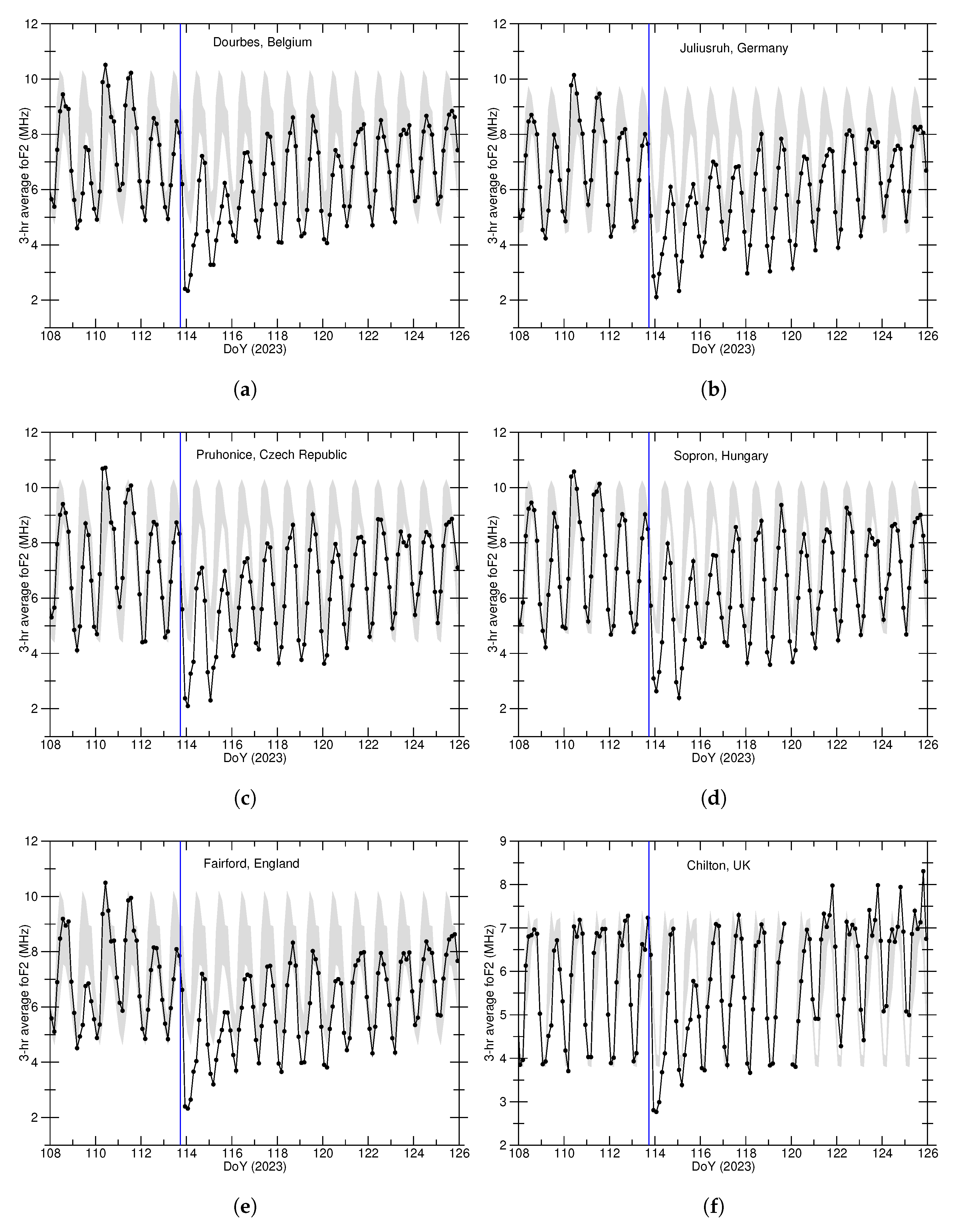
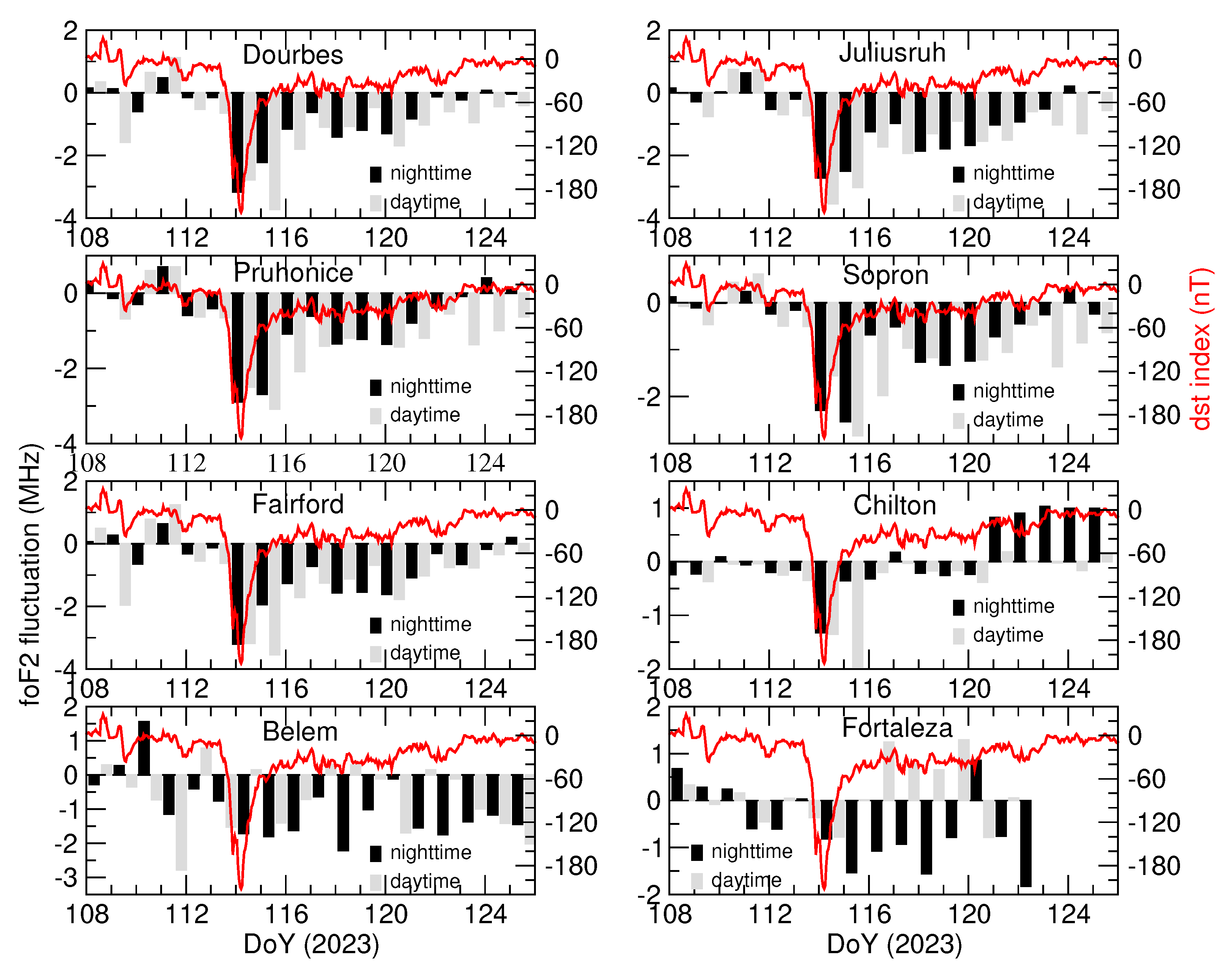
3.2. Variation of foF2

The 3-hour average of foF2 values, obtained through the auto-scaling of the Digisonde GIRO measurements (https://giro.uml.edu (accessed on 13 July 2024)), is plotted in Figure 8 for six European stations: Dourbes, Belgium; Juliusruh, Germany; Pruhonice, Czech Republic; Sopron, Hungary; Fairford, England; and Chilton, UK. These ionosonde stations are located close to the SuperSID VLF/LF receivers we are studying in this paper. The deviation of foF2 beyond the 2 σ level from the normal values is evident. The maximum variation in foF2 1 2 MHz for all six stations was observed on April 23 (DoY 114), coinciding with the peak of the storm. Another significant variation in foF2 was recorded on April 24, when the k p index reached 8+ and the Dst index reached its minimum. The substantial variations in the average foF2 values persisted for 7–8 days following the storm’s onset on April 23. The gray region in all figures represents the mean of the 3-hour average foF2 values of the pre-storm days (April 18–22) ± σ .
Figure 9 shows the variation of the 3-hour average of foF2 values recorded at two ionosonde stations in South America: Belem and Fortaleza in Brazil. These stations are situated in the equatorial region and near the Stanford VLF receiver at UTP, Colombia. The Digisonde stations closest to UTP, Colombia, did not have data during the study period from 18 April to 5 May 2023 (DoY 108–126). The station at Fortaleza, Brazil, has data available between 18 April and 2 May 2023, which is sufficient for our analysis. The analysis of the 3-hour average values of foF2 shows no significant variation at the Digisonde stations located in Belem and Fortaleza, Brazil, during the storm-disturbed period. This observation aligns with the absence of significant variation in the VLF/LF data at UTP, Colombia, during the storm period.
We present the 3-hour average fluctuations of both daytime and nighttime foF2 values in Figure 10. The fluctuations were calculated by subtracting the mean of the 3-hour foF2 values from the pre-storm days (April 18–22) from the corresponding 3-hour average foF2 values for each day during the study period (DoY 108–125). In each plot, black bars represent nighttime foF2 deviations, computed over a 3-hour interval (0–3 UT for European Digisonde stations and 3–6 UT for Brazilian stations). Gray bars indicate daytime foF2 deviations, calculated over a 3-hour interval (12–15 UT for European stations and 15–18 UT for Brazilian stations). The red curve overlaid on each plot shows the variation of the Dst index throughout the study period. Significant daytime and nighttime foF2 fluctuations, up to approximately 3 MHz, were observed at the mid-latitude Digisonde stations in Dourbes, Juliusruh, Pruhonice, Sopron, Fairford, and Chilton. The maximum deviations occurred after the beginning of the geomagnetic storm and during its peak phase from April 23 to 25 (DoY 113–115). However, the variations observed at the low-latitude stations in Belem and Fortaleza were not significant.

4. Discussions and Conclusions

In this study, we aimed to determine how the severe geomagnetic storm of April 2023 impacted the lower and upper ionosphere in the low-to-middle latitude regions by analyzing VLF signals that probe the lower ionosphere and ionosonde data of foF2, which gives information about the upper ionosphere. However, the VLF signals show path-dependent variations influenced by ionospheric conditions along the propagation path in the Earth Ionosphere Waveguide [43]. Ionosonde data, obtained from high-frequency (HF) signals transmitted upward and reflected from the upper ionosphere, provide a localized measurement of upper ionospheric response [44]. The storm is clearly evident in Figure 1, where the K p index reached 8+ twice on April 23 and April 24 and remained high throughout the storm period. The Dst index also dropped below −100 nT on April 23, reaching a minimum of −212 nT, further indicating the intensity of the storm. In brief, our findings are as follows:
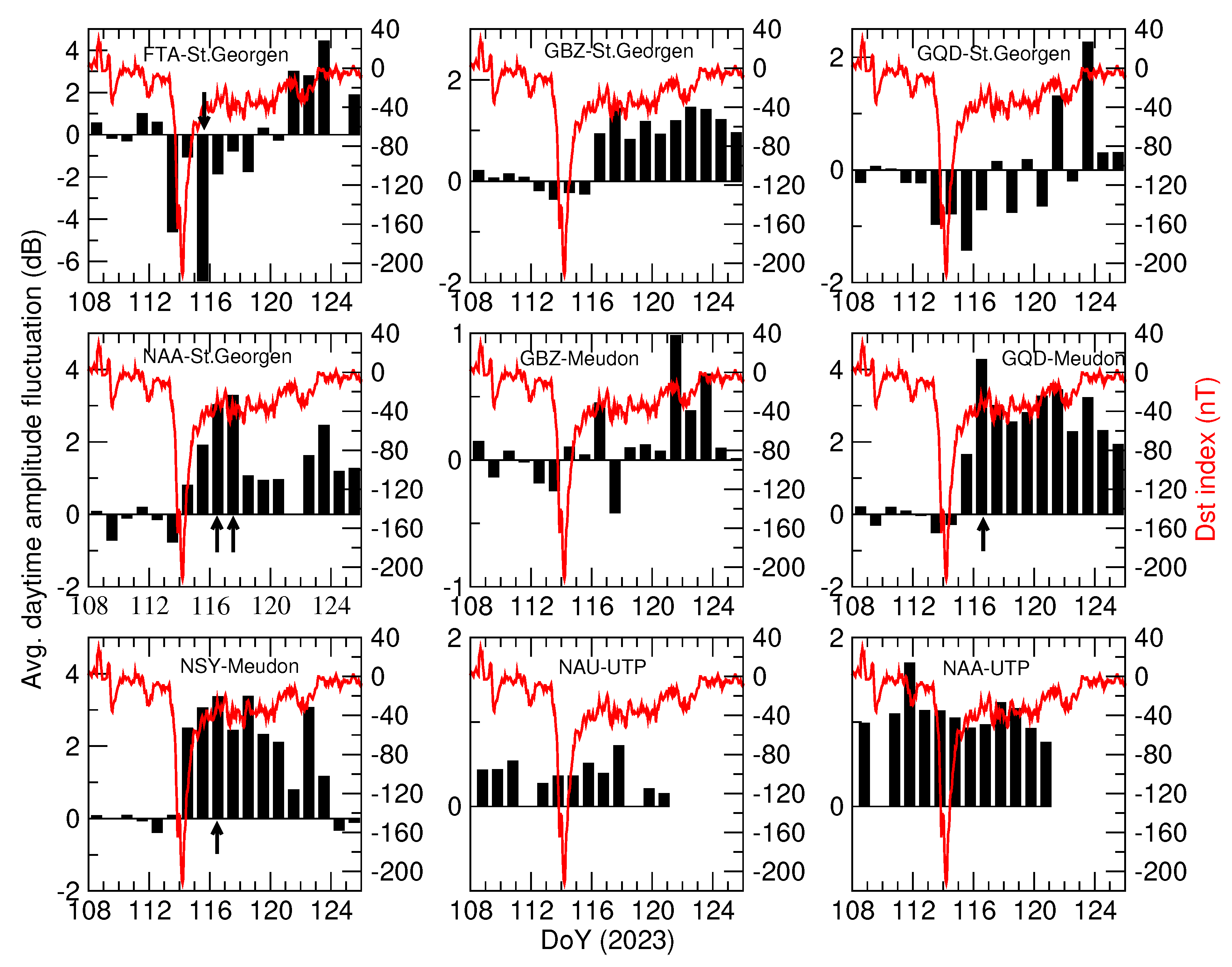
  • The mid-latitude VLF/LF propagation paths considered in this study exhibit varying degrees of response to the superstorm of 23 April 2023. The variations of VLF signals along different paths may depend on several factors. Even minor differences in their Great Circle Paths, transmitting powers, and initial launch angles could lead to variations in how they are affected by ionospheric disturbances.
  • In the short propagation paths, higher-frequency LF signals (FTA: 63.85 kHz and NSY: 45.9 kHz) show stronger perturbations compared to VLF signals (3–30 kHz). LF signals are attenuated (∼3–5 dB) throughout the daytime, while VLF signals are only affected during the sunrise and sunset period (Figure 3b,d). The GBZ-St. Georgen path (GBZ: 19.58 kHz) exhibits relatively lower noise compared to FTA-St. Georgen, likely due to differences in ionospheric interaction heights and propagation characteristics.
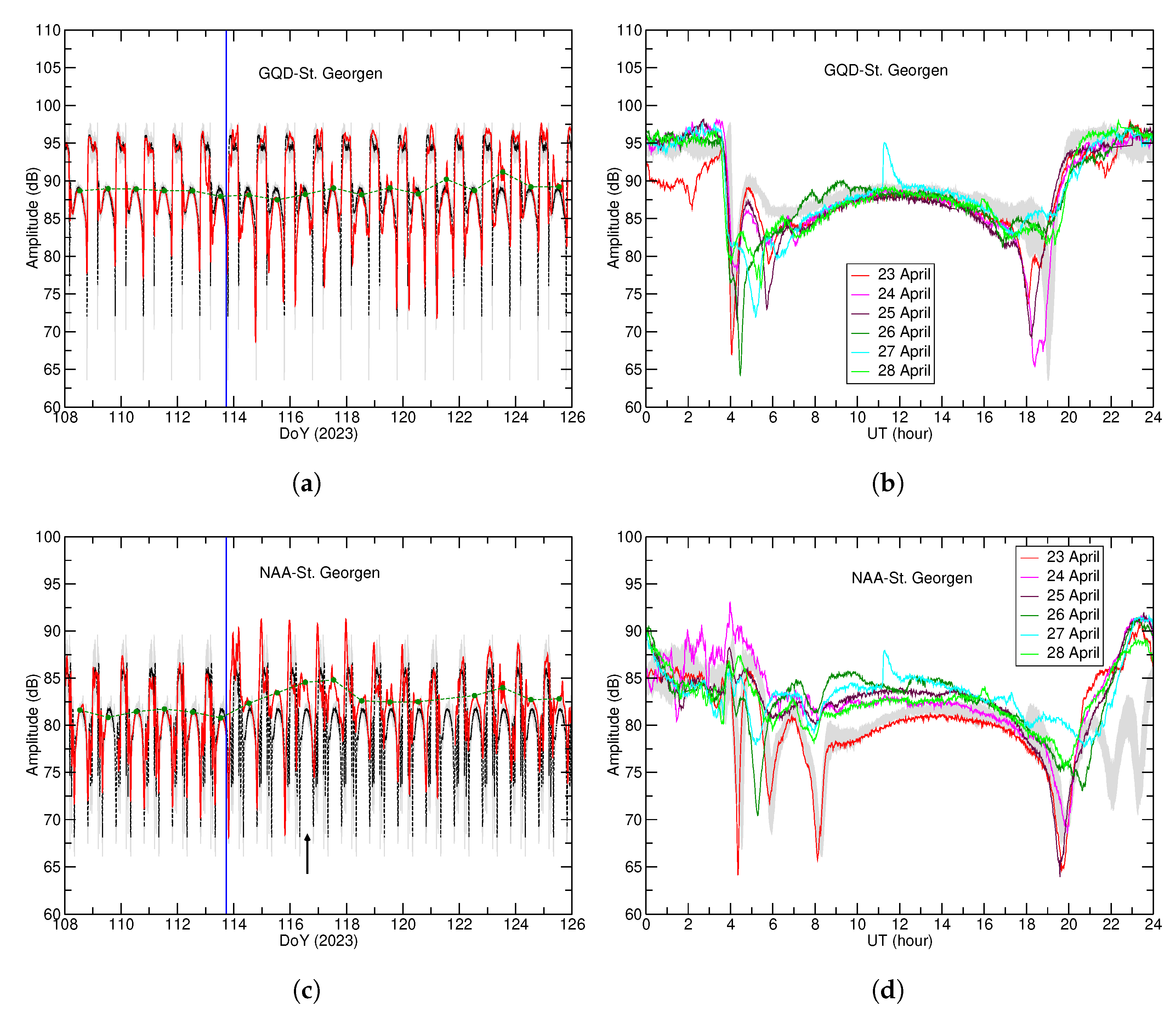
  • VLF signals exhibit stronger variations in the post-storm period along the long trans-oceanic paths over the mid-latitude region compared to long propagation paths in the low-latitude region. The level of disturbance is influenced by the latitude of the receiving station and the strength of geomagnetic disturbances along the path. For instance, despite both being long paths, NAA-St. Georgen (5500 km, mid-latitude) shows stronger perturbations than NAA-UTP (4450 km, low-latitude) due to the greater impact of geomagnetic disturbances at mid-latitudes.
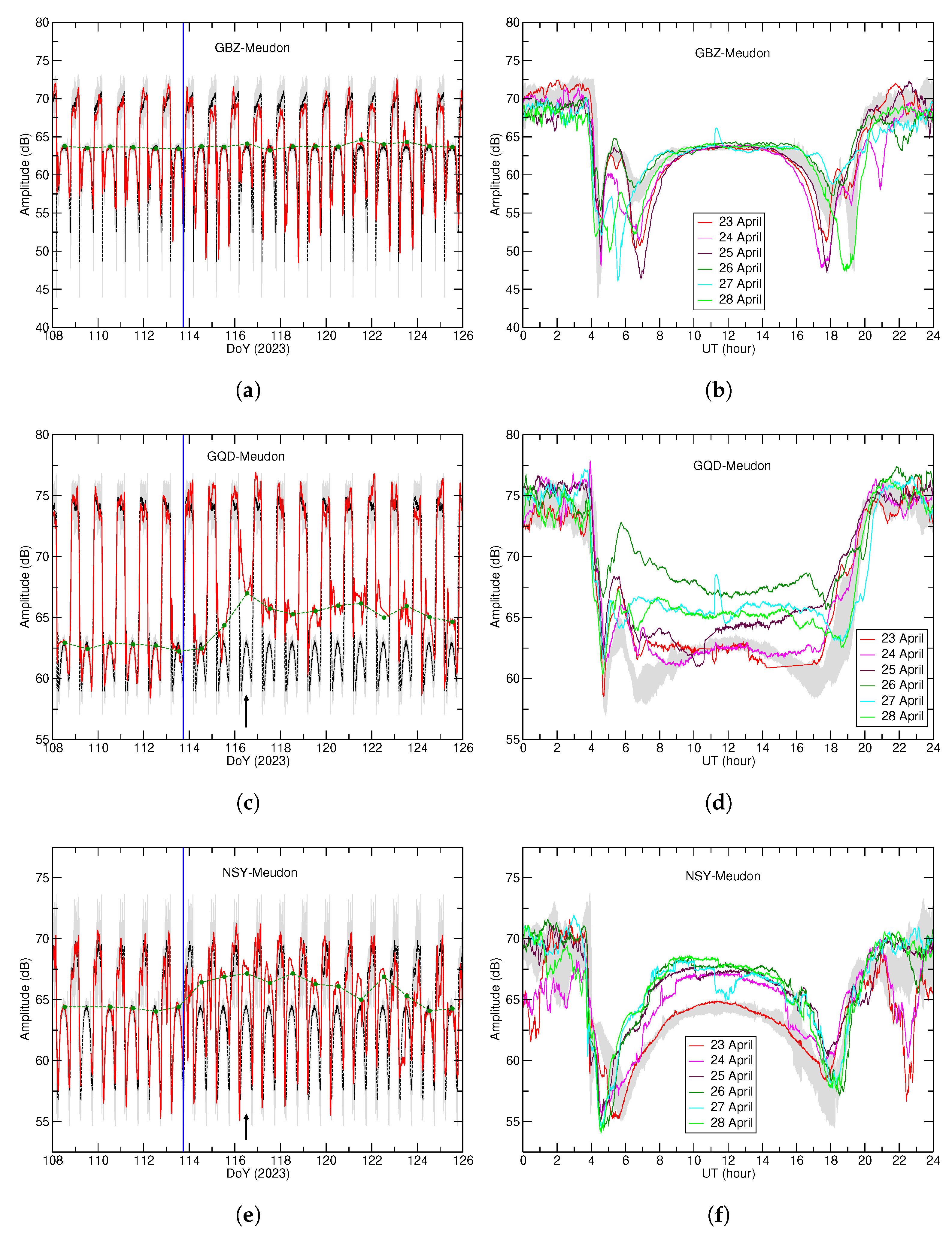
  • Both the transmitters, GBZ (19.58 kHz) and GQD (22.1 kHz), are located close to each other in the UK, and VLF signals from both received at Meudon show different behavior in diurnal variations. The variation in daytime signals along GQD–Meudon is more prominent. These differences can happen due to minor differences in their Great Circle Paths, transmitting powers, and initial launch angles of the signals, which could lead to signal variations, as observed along the two paths affected by ionospheric disturbances. The ionospheric reflection height and electron density variations may differ slightly for each frequency, which can further lead to differences in the observed signal deviation.
  • The 2-hour mid-day average signal amplitudes deviated by approximately (∼3–5 dB) from the average quiet-day signals (see Figure 7). This deviation was observed consistently in the time-series plots of multiple propagation paths, including FTA-St. Georgen (Figure 3a), NAA-St. Georgen (Figure 4c), GQD-Meudon (Figure 5c), and NSY-Meudon (Figure 5e).
  • No significant variation of VLF/LF signals is observed in the long or short path propagation paths in the low latitudes (Figure 6b,d), corroborating Tatsuta et al. [33]. The storm-induced signatures may not always be straightforward; the 2-hour midday average plot indicated by green circles connected by green dotted lines in Figure 6a,c remained straight, which supports our statement that no significant perturbations were observed along these paths.
  • Fluctuation in the 3-hour averaged foF2 value in the mid-latitude crossed 2 σ level on 23 and 24 April, indicating upper ionospheric disturbances during the storm (Figure 8) for a prolonged period. Both daytime and nighttime values of foF2 varied up to ∼3 MHz at the mid-latitude Digisonde stations (see Figure 10). Again, no considerable change in foF2 has been observed in the low-latitude ionosonde stations.
  • The peak variation of VLF/LF signals is observed on April 25–26 (DoY 115–116), as indicated by black arrows in Figure 3, Figure 4 and Figure 5 and Figure 7. The black arrows are not indicated in Figure 4a, Figure 5a, and Figure 6a,c, since significant deviation could not be determined from the plot. The fluctuation of foF2 variation at the mid-latitude region peaked shortly after the commencement of the storm, indicating a faster response of the F-region ionosphere to the geomagnetic storm.
  • There is a difference in noise levels between the NAU–UTP (LF, 40.8 kHz) and NAA–UTP (VLF, 24.0 kHz) paths during the night interval. LF signals (such as the 40.8 kHz NAU signal) experience higher attenuation due to interactions with the lower ionosphere (D-region) during nighttime, leading to increased signal fluctuations. In contrast, VLF signals (24.0 kHz from NAA) are less affected by such variations and can maintain more stable propagation conditions.
  • In the mid-latitude, prominent ionospheric disturbances have been detected in both the lower and upper ionosphere.
The variations of VLF signals are influenced by multiple factors, including the length of the Great Circle Path, whether the path is over ocean or land, the direction of the path, the transmitting frequency, and the latitude of the receiving station. The amplitude deviations are particularly prominent during the daytime due to increased ionization from solar X-ray and EUV radiation, coupled with storm-induced electric fields and particle precipitation, which affect the D-region ionosphere, where VLF/LF signals reflect. Paths such as FTA–DE_St_Georgen (Figure 3b), GBZ–DE_St_Georgen (Figure 3d), GQD–DE_St_Georgen (Figure 4b), and NAA–DE_St_Georgen (Figure 4d) show significant daytime variations, with GBZ–DE_St_Georgen and GQD–DE_St_Georgen showing decreased terminator signals, both at Sunrise Terminator Time (SRT) and Sunset Terminator Time (SST). Nighttime signal variations were observed predominantly after sunset on several paths, particularly for mid-latitude propagation paths like GBZ–DE_St_Georgen, GQD-DE_St_Georgen, and NAA–DE_St_Georgen. Nighttime VLF radio signal disturbances can also result from various phenomena beyond geomagnetic storms, including intense lightning discharges [34,35], which can cause disturbances lasting from a few seconds to several minutes, as well as earthquakes [45,46,47] and sudden stratospheric warming (SSW) events [36,37]. Strong earthquakes and sudden stratospheric warming (SSW) events, in particular, can produce nighttime disturbances similar to those observed in this study. Hayakawa and Molchanov [46], Pulinets and Davidenko [48] reported ionospheric perturbations occurring days before large earthquakes, attributed to lithosphere–atmosphere–ionosphere coupling, but these anomalies are often observed as gradual changes in signal amplitude and thus differ from the abrupt fluctuations seen in geomagnetic storms. However, during the analysis period, there were no recorded earthquakes near the propagation path, as verified using global earthquake databases (https://www.usgs.gov (accessed on 15 February 2025)). For SSW events, ionospheric disturbances are typically characterized by long-duration variations in foF2 and VLF signal perturbations extending over several days to weeks due to planetary wave activity [49]. Since no SSW events occurred during our analysis period, these effects can be ruled out. Thus, the nighttime variations of the VLF signals could be due to persistent particle precipitation and residual ionospheric disturbances from the storm, leading to fluctuations in the D-region electron density [11,50]. The daytime signal was analyzed in more detail because daytime ionospheric disturbances tend to be more prominent in mid-latitudes due to direct solar forcing. Nwankwo et al. [51] reported disturbances in daytime signals in the mid-latitude region during 80% of the storm events considered in their study.
The fluctuations in VLF/LF signal amplitudes during the storm period are mainly caused by waveguide modal interference effects among various propagating modes within the Earth ionosphere waveguide modified due to the storm. The increase or decrease in signal amplitude depends on the type of interference, whether it is constructive or destructive. These effects are more significant in long paths, as they allow signals to interact with disturbed regions of the ionosphere over an extended distance and time, making them more sensitive to geomagnetic perturbations [43]. The long-distance trans-oceanic west-to-east NAA–DE_St_Georgen path showed prominent variation in both day and nighttime signals. The attenuation of VLF signals is lower over the Atlantic surface, due to the uniform conductivity of the oceanic surface, making the propagation path well suited for the detection of geomagnetic-storm-induced perturbation, which is evident from Figure 4d. Due to multiple interactions with the ionosphere in the EIWG along a long path, the signals could show a prominent variation at night, particularly after sunset.
The visibility of geomagnetic storm effects on VLF/LF signals is strongly modulated by the baseline ionization levels, which are dominated by solar radiation during the day, and propagation path lengths. Due to the absence of the Sun, various factors control the VLF reflection heights that fluctuate randomly, leading to greater variability of the nighttime VLF signals. The day-to-day nighttime variability can mask or minimize the effects of geomagnetic storms on some VLF/LF signals such as the signals along the GBZ–Meudon path (Figure 5b) and the GQD–Meudon path (Figure 5d), making such changes less visible or difficult to detect during nighttime.
The peak variation of VLF/LF signals along different propagation paths was observed 2–3 days after the occurrence of the storm. The delay in the peak disturbance of VLF signals during the superstorm of March 2015 was reported by Mondal et al. [11]. In the aftermath of a geomagnetic storm, there is a time-lapse in the precipitation of energetic charged particles in the lower ionosphere (D-layer) that is responsible for VLF/LF wave disturbance. The ionization process in the lower ionosphere is slower due to slower chemical reactions and faster recombination processes, which lead to a delayed response by the VLF/LF signals [52]. Geomagnetic storms generate atmospheric gravity waves (AGWs) and Traveling Ionospheric Disturbances (TIDs) that propagate downward, affecting the the D-region ionospheric density, which in turn affects the VLF wave propagation [53]. However, the downward propagation of the AGWs and TIDs takes time, which contributes to the delay observed by VLF/LF signals.
Major geomagnetic storms can significantly change the density, composition, and circulation of the ionosphere–thermosphere system on a global scale. These changes often persist for several days even after the geomagnetic activity has subsided. Geomagnetic storms can cause thermospheric changes such as heating in the thermosphere and an increase in the thermospheric wind speed, leading to changes in the neutral atmosphere’s composition, particularly in the atomic oxygen-to-nitrogen ratio ( O / N 2 ) [54]. The decrease in foF2 values during the April 2023 geomagnetic storm is caused by the depletion of peak electron content due to the reduction in the O / N 2 ratio [55]. Such negative variation of foF2 during the geomagnetic storm of April 2023 indicates a strong negative ionospheric storm [23]. Oikonomou et al. [22], attributed the sharp decline in electron density (in terms of foF2) over the European sector during the geomagnetic storm in September 2017 to the displacement of the MIT coupled with TIDs. The MIT region is characterized by a decrease in ionospheric plasma density in the F2 layer and typically forms at mid-latitudes. During the geomagnetic storm of April 2023, the MIT deepened, indicating a reduction in electron density, and shifted in latitude, causing more significant reductions in foF2 over the European region.

Author Contributions

Conceptualization, A.S. and S.P.; methodology, A.S., S.P. and S.K.M.; formal analysis, A.S.; investigation, A.S., S.P. and S.K.M.; resources, A.S. and B.D.; writing—original draft preparation, A.S. and S.P.; writing—review and editing, A.S., S.P. and S.K.M.; supervision, S.P. and S.K.M. All authors have read and agreed to the published version of the manuscript.

Funding

This research received no external funding.

Institutional Review Board Statement

Not applicable.

Informed Consent Statement

Not applicable.

Data Availability Statement

The VLF/LF data was obtained from the Space Weather Monitors at the Stanford SOLAR Center (http://sid.stanford.edu/database-browser/ (accessed on 6 June 2023)). The K p and Dst indices were sourced from the World Data Center for Geomagnetism, Kyoto (https://wdc.kugi.kyoto-u.ac.jp (accessed on 7 December 2023)). The foF2 data was acquired from the ionosonde ionogram measurements at the Digisonde Global Ionosphere Radio Observatory (GIRO) by Lowell Digisonde International (https://giro.uml.edu/didbase/ (accessed on 13 July 2024)).

Acknowledgments

The authors acknowledge the Stanford SuperSID project, WDC, Kyoto and Digisonde for using their data in this paper. A. Sen acknowledges the support of NERIE-NCERT, Shillong for extending opportunity to undertake this work.

Conflicts of Interest

The authors declare no conflicts of interest.

References

  1. Gonzalez, W.D.; Joselyn, J.A.; Kamide, Y.; Kroehl, H.W.; Rostoker, G.; Tsurutani, B.T.; Vasyliunas, V.M. What is a geomagnetic storm? J. Geophys. Res. Space Phys. 1994, 99, 5771–5792. [Google Scholar] [CrossRef]
  2. Ghag, K.; Raghav, A.; Bhaskar, A.; Soni, S.L.; Sathe, B.; Shaikh, Z.; Dhamane, O.; Tari, P. Quasi-planar ICME sheath: A cause of the first two-step extreme geomagnetic storm of the 25th solar cycle observed on 23 April 2023. Adv. Space Res. 2024, 73, 6288–6297. [Google Scholar] [CrossRef]
  3. Chapman, S.; Bartels, J. Geomagnetism, Vol. II: Analysis of the Data, and Physical Theories; Oxford University Press: Oxford, UK, 1940. [Google Scholar]
  4. Gonzalez, W.D.; Tsurutani, B.T.; Clúa de Gonzalez, A.L. Interplanetary origin of geomagnetic storms. Space Sci. Rev. 1999, 88, 529–562. [Google Scholar] [CrossRef]
  5. Baruah, Y.; Roy, S.; Sinha, S.; Palmerio, E.; Pal, S.; Oliveira, D.M.; Nandy, D. The Loss of Starlink Satellites in February 2022: How Moderate Geomagnetic Storms Can Adversely Affect Assets in Low-Earth Orbit. Space Weather 2024, 22, e2023SW003716. [Google Scholar] [CrossRef]
  6. Parks, G. MAGNETOSPHERE. In Encyclopedia of Atmospheric Sciences; Holton, J.R., Ed.; Academic Press: Oxford, UK, 2003; pp. 1229–1237. [Google Scholar] [CrossRef]
  7. Kivelson, M.G.; Bagenal, F. Chapter 28—Planetary Magnetospheres. In Encyclopedia of the Solar System, 2nd ed.; McFadden, L.A., Weissman, P.R., Johnson, T.V., Eds.; Academic Press: San Diego, CA, USA, 2007; pp. 519–540. [Google Scholar] [CrossRef]
  8. Chenette, D.L.; Datlowe, D.W.; Robinson, R.M.; Schumaker, T.L.; Vondrak, R.R.; Winningham, J.D. Atmospheric energy input and ionization by energetic electrons during the geomagnetic storm of 8–9 November 1991. Geophys. Res. Lett. 1993, 20, 1323–1326. [Google Scholar] [CrossRef]
  9. Laštovička, J. Effects of geomagnetic storms in the lower ionosphere, middle atmosphere and troposphere. J. Atmos. Terr. Phys. 1996, 58, 831–843. [Google Scholar] [CrossRef]
  10. Sokolov, S.N. Magnetic storms and their effects in the lower ionosphere: Differences in storms of various types. Geomagn. Aeron. 2011, 51, 741–752. [Google Scholar] [CrossRef]
  11. Mondal, S.K.; Pal, S.; Sen, A.; Rahaman, M.; Midya, S.K. Long-lasting disturbances in the mid-latitude sub-ionospheric VLF radio signals due to the super geomagnetic storm of 17 March 2015. Adv. Space Res. 2021, 68, 2295–2308. [Google Scholar] [CrossRef]
  12. WMO. International Meteorological Vocabulary; World Meteorological Organization: Geneva, Switzerland, 1992. [Google Scholar]
  13. Fagundes, P.R.; Cardoso, F.A.; Fejer, B.G.; Venkatesh, K.; Ribeiro, B.A.G.; Pillat, V.G. Positive and negative GPS-TEC ionospheric storm effects during the extreme space weather event of March 2015 over the Brazilian sector. J. Geophys. Res. Space Phys. 2016, 121, 5613–5625. [Google Scholar] [CrossRef]
  14. Prölss, G. On explaining the negative phase of ionospheric storms. Planet. Space Sci. 1976, 24, 607–609. [Google Scholar] [CrossRef]
  15. Ratovsky, K.G.; Klimenko, M.V.; Yasyukevich, Y.V.; Klimenko, V.V.; Vesnin, A.M. Statistical Analysis and Interpretation of High-, Mid- and Low-Latitude Responses in Regional Electron Content to Geomagnetic Storms. Atmosphere 2020, 11, 1308. [Google Scholar] [CrossRef]
  16. Prölss, G. Ionospheric F-Region Storms: Unsolved Problems. In Characterising the Ionosphere; Meeting Proceedings RTO-MP-IST-056; Paper 10; RTO: Neuilly-sur-Seine, France, 2006; pp. 10-1–10-20. [Google Scholar]
  17. Frissell, N.A.; Kaeppler, S.R.; Sanchez, D.F.; Perry, G.W.; Engelke, W.D.; Erickson, P.J.; Coster, A.J.; Ruohoniemi, J.M.; Baker, J.B.H.; West, M.L. First Observations of Large Scale Traveling Ionospheric Disturbances Using Automated Amateur Radio Receiving Networks. Geophys. Res. Lett. 2022, 49, e2022GL097879. [Google Scholar] [CrossRef]
  18. Thaganyana, G.P.; Habarulema, J.B.; Ngwira, C.; Azeem, I. Equatorward Medium to Large-Scale Traveling Ionospheric Disturbances of High Latitude Origin During Quiet Conditions. J. Geophys. Res. Space Phys. 2022, 127, e2021JA029558. [Google Scholar] [CrossRef]
  19. Rodger, A.; Moffett, R.; Quegan, S. The role of ion drift in the formation of ionisation troughs in the mid- and high-latitude ionosphere—A review. J. Atmos. Terr. Phys. 1992, 54, 1–30. [Google Scholar] [CrossRef]
  20. Prölss, G.W.; Brace, L.H.; Mayr, H.G.; Carignan, G.R.; Killeen, T.L.; Klobuchar, J.A. Ionospheric storm effects at subauroral latitudes: A case study. J. Geophys. Res. Space Phys. 1991, 96, 1275–1288. [Google Scholar] [CrossRef]
  21. Nayak, C.; Tsai, L.C.; Su, S.Y.; Galkin, I.A.; Tan, A.T.K.; Nofri, E.; Jamjareegulgarn, P. Peculiar features of the low-latitude and midlatitude ionospheric response to the St. Patrick’s Day geomagnetic storm of 17 March 2015. J. Geophys. Res. Space Phys. 2016, 121, 7941–7960. [Google Scholar] [CrossRef]
  22. Oikonomou, C.; Haralambous, H.; Paul, A.; Ray, S.; Alfonsi, L.; Cesaroni, C.; Sur, D. Investigation of the negative ionospheric response of the 8 September 2017 geomagnetic storm over the European sector. Adv. Space Res. 2022, 70, 1104–1120. [Google Scholar] [CrossRef]
  23. Habarulema, J.B.; Zhang, Y.; Matamba, T.; Buresova, D.; Lu, G.; Katamzi-Joseph, Z.; Fagundes, P.R.; Okoh, D.; Seemala, G. Absence of High Frequency Echoes From Ionosondes During the 23–25 April 2023 Geomagnetic Storm; What Happened? J. Geophys. Res. Space Phys. 2024, 129, e2023JA032277. [Google Scholar] [CrossRef]
  24. Davies, K. Ionospheric Radio; Electromagnetic Waves; Institution of Engineering and Technology: Stevenage, UK, 1990. [Google Scholar] [CrossRef]
  25. Mitra, A.P. Ionospheric Effects of Solar Flares; Springer: Dordrecht, The Netherlands, 1974; Volume 46. [Google Scholar] [CrossRef]
  26. Clilverd, M.A.; Rodger, C.J.; Thomson, N.R.; Lichtenberger, J.; Steinbach, P.; Cannon, P.; Angling, M.J. Total solar eclipse effects on VLF signals: Observations and modeling. Radio Sci. 2001, 36, 773–788. [Google Scholar] [CrossRef]
  27. Davorka, G.; Šulić, D.; Žigman, V. Influence of solar X-ray flares on the earth-ionosphere waveguide. Serbian Astron. J. 2005, 171, 29–35. [Google Scholar] [CrossRef]
  28. Pal, S.; Chakrabarti, S.K.; Mondal, S.K. Modeling of sub-ionospheric VLF signal perturbations associated with total solar eclipse, 2009 in Indian subcontinent. Adv. Space Res. 2012, 50, 196–204. [Google Scholar] [CrossRef]
  29. Pal, S.; Maji, S.K.; Chakrabarti, S.K. First ever VLF monitoring of the lunar occultation of a solar flare during the 2010 annular solar eclipse and its effects on the D-region electron density profile. Planet. Space Sci. 2012, 73, 310–317. [Google Scholar] [CrossRef]
  30. Mondal, S.K.; Chakrabarti, S.K.; Sasmal, S. Detection of ionospheric perturbation due to a soft gamma ray repeater SGR J1550-5418 by very low frequency radio waves. Astrophys. Space Sci. 2012, 341, 259–264. [Google Scholar] [CrossRef]
  31. Belrose, J.; Thomas, L. Ionization changes in the middle lattitude D-region associated with geomagnetic storms. J. Atmos. Terr. Phys. 1968, 30, 1397–1413. [Google Scholar] [CrossRef]
  32. Kikuchi, T.; Evans, D.S. Quantitative study of substorm-associated VLF phase anomalies and precipitating energetic electrons on November 13, 1979. J. Geophys. Res. Space Phys. 1983, 88, 871–880. [Google Scholar] [CrossRef]
  33. Tatsuta, K.; Hobara, Y.; Pal, S.; Balikhin, M. Sub-ionospheric VLF signal anomaly due to geomagnetic storms: A statistical study. Ann. Geophys. 2015, 33, 1457–1467. [Google Scholar] [CrossRef]
  34. Inan, U.S.; Shafer, D.C.; Yip, W.Y.; Orville, R.E. Subionospheric VLF signatures of nighttime D region perturbations in the vicinity of lightning discharges. J. Geophys. Res. Space Phys. 1988, 93, 11455–11472. [Google Scholar] [CrossRef]
  35. Hobara, Y.; Iwasaki, N.; Hayashida, T.; Hayakawa, M.; Ohta, K.; Fukunishi, H. Interrelation between ELF transients and ionospheric disturbances in association with sprites and elves. Geophys. Res. Lett. 2001, 28, 935–938. [Google Scholar] [CrossRef]
  36. Pal, S.; Hobara, Y.; Chakrabarti, S.K.; Schnoor, P.W. Effects of the major sudden stratospheric warming event of 2009 on the subionospheric very low frequency/low frequency radio signals. J. Geophys. Res. Space Phys. 2017, 122, 7555–7566. [Google Scholar] [CrossRef]
  37. Sen, A.; Pal, S.; Mondal, S.K. Mid-latitude ionospheric disturbances during the major Sudden Stratospheric Warming event of 2018 observed by sub-ionospheric VLF/LF signals. Adv. Space Res. 2024, 73, 767–779. [Google Scholar] [CrossRef]
  38. Iijima, T.; Potemra, T.A. The amplitude distribution of field-aligned currents at northern high latitudes observed by Triad. J. Geophys. Res. (1896-1977) 1976, 81, 2165–2174. [Google Scholar] [CrossRef]
  39. Matzka, J.; Stolle, C.; Yamazaki, Y.; Bronkalla, O.; Morschhauser, A. The Geomagnetic Kp Index and Derived Indices of Geomagnetic Activity. Space Weather 2021, 19, e2020SW002641. [Google Scholar] [CrossRef]
  40. Borovsky, J.E.; Shprits, Y.Y. Is the Dst Index Sufficient to Define All Geospace Storms? J. Geophys. Res. Space Phys. 2017, 122, 11,543–11,547. [Google Scholar] [CrossRef]
  41. Gonzalez, W.; Tsurutani, B.; Clúa de Gonzalez, A. Geomagnetic storms contrasted during solar maximum and near solar minimum. Adv. Space Res. 2002, 30, 2301–2304. [Google Scholar] [CrossRef]
  42. Barman, K.; Adhikary, S.; Das, B.; Pal, S.; Haldar, P.K. Low-latitude sub-ionospheric VLF radio signal disturbances due to solar flares: Effects on the attenuation and phase velocities of the waveguide modes. J. Atmos. Sol.-Terr. Phys. 2025, 268, 106433. [Google Scholar] [CrossRef]
  43. Thomson, N.R.; Rodger, C.J.; Clilverd, M.A. Daytime D region parameters from long-path VLF phase and amplitude. J. Geophys. Res. Space Phys. 2011, 116, A11305. [Google Scholar] [CrossRef]
  44. Fung, S.F.; Benson, R.F.; Galkin, I.A.; Green, J.L.; Reinisch, B.W.; Song, P.; Sonwalkar, V. Chapter 4—Radio-frequency imaging techniques for ionospheric, magnetospheric, and planetary studies. In Understanding the Space Environment Through Global Measurements; Colado-Vega, Y., Gallagher, D., Frey, H., Wing, S., Eds.; Elsevier: Amsterdam, The Netherlands, 2022; pp. 101–216. [Google Scholar] [CrossRef]
  45. Molchanov, O.A.; Hayakawa, M. Subionospheric VLF signal perturbations possibly related to earthquakes. J. Geophys. Res. Space Phys. 1998, 103, 17489–17504. [Google Scholar] [CrossRef]
  46. Hayakawa, M.; Molchanov, O. Effect of earthquakes on lower ionosphere as found by subionospheric VLF propagation. Adv. Space Res. 2000, 26, 1273–1276. [Google Scholar] [CrossRef]
  47. Das, B.; Sen, A.; Haldar, P.K.; Pal, S. VLF radio signal anomaly associated with geomagnetic storm followed by an earthquake at a subtropical low latitude station in northeastern part of India. Indian J. Phys. 2022, 96, 13–24. [Google Scholar] [CrossRef]
  48. Pulinets, S.; Davidenko, D. Ionospheric precursors of earthquakes and Global Electric Circuit. Adv. Space Res. 2014, 53, 709–723. [Google Scholar] [CrossRef]
  49. Goncharenko, L.P.; Coster, A.J.; Chau, J.L.; Valladares, C.E. Impact of sudden stratospheric warmings on equatorial ionization anomaly. J. Geophys. Res. Space Phys. 2010, 115, A00G07. [Google Scholar] [CrossRef]
  50. Rodger, C.J.; Clilverd, M.A.; Thomson, N.R.; Gamble, R.J.; Seppälä, A.; Turunen, E.; Meredith, N.P.; Parrot, M.; Sauvaud, J.A.; Berthelier, J.J. Radiation belt electron precipitation into the atmosphere: Recovery from a geomagnetic storm. J. Geophys. Res. Space Phys. 2007, 112, A11307. [Google Scholar] [CrossRef]
  51. Nwankwo, V.U.J.; Denig, W.; Chakrabarti, S.K.; Ogunmodimu, O.; Ajakaiye, M.P.; Fatokun, J.O.; Anekwe, P.I.; Obisesan, O.E.; Oyanameh, O.E.; Fatoye, O.V. Diagnostic study of geomagnetic storm-induced ionospheric changes over very low-frequency signal propagation paths in the mid-latitude D region. Ann. Geophys. 2022, 40, 433–461. [Google Scholar] [CrossRef]
  52. Prölss, G.W. Physics of the Earth’s Space Environment: An Introduction; Springer: Berlin/Heidelberg, Germany, 2004. [Google Scholar] [CrossRef]
  53. Maurya, A.K.; Venkatesham, K.; Kumar, S.; Singh, R.; Tiwari, P.; Singh, A.K. Effects of St. Patrick’s Day Geomagnetic Storm of March 2015 and of June 2015 on Low-Equatorial D Region Ionosphere. J. Geophys. Res. Space Phys. 2018, 123, 6836–6850. [Google Scholar] [CrossRef]
  54. Schunk, R.W.; Nagy, A.F. Ionospheres: Physics, Plasma Physics, and Chemistry; Cambridge University Press: Cambridge, UK, 2009. [Google Scholar]
  55. Yue, X.; Wang, W.; Lei, J.; Burns, A.; Zhang, Y.; Wan, W.; Liu, L.; Hu, L.; Zhao, B.; Schreiner, W.S. Long-lasting negative ionospheric storm effects in low and middle latitudes during the recovery phase of the 17 March 2013 geomagnetic storm. J. Geophys. Res. Space Phys. 2016, 121, 9234–9249. [Google Scholar] [CrossRef]
Figure 1. Variation of K p (top panel) and Dst index (bottom panel) during 15 April–10 May 2023 (Day of Year (DoY) 105–130). K p reached 8 + and Dst reached −212 nT on 23–24 April 2023, indicating a severe geomagnetic storm. The red vertical line marks the time when the storm initiated. Data source: World Data Center for Geomagnetism, Kyoto (https://wdc.kugi.kyoto-u.ac.jp (accessed on 7 December 2023)).
Atmosphere 16 00716 g001
Figure 2. Great Circle Paths (GCPs) between the transmitters and receivers are represented by blue lines. All the transmitters (red dots), receivers (green dots) and Digisonde stations (violet stars) considered in this study are marked.
Atmosphere 16 00716 g002
Figure 3. (a,c): Time series plot (red) of diurnal variations of VLF/LF signals from transmitters FTA and GBZ received at De_St_Georgen, Germany. VLF/LF data, exhibiting diurnal variations for each propagation path, were downloaded from the Stanford SuperSID monitors’ database. The blue vertical line marks the time when the storm initiated on April 23 (DoY 113). The black dashed curve indicates the average signal amplitude of pre-storm days. Green circles (connected by green dotted lines) represent the daytime average values computed over a 2-hour interval (12–14 UT) around mid-day. The gray shade in all figures represents the average signal amplitude of pre-storm days (April 18–22) ± 2 σ . The black arrows indicate the peak variations of signal amplitude. (b,d): The diurnal variations of VLF/LF signals from FTA and GBZ on storm-disturbed days (April 23–28, DoY 113–118).
Atmosphere 16 00716 g003
Figure 4. (a,c): Time series plot (red) of diurnal variations of VLF signals from transmitters GQD and NAA received at De_St_Georgen, Germany. The blue vertical line marks the time when the storm initiated on April 23 (DoY 113). The black dashed curve indicates the average signal amplitude of pre-storm days. Green circles (connected by green dotted lines) represent the daytime average values computed over a 2-hour interval (12–14 UT) around mid-day. The gray shade in all figures represents the average signal amplitude of pre-storm days (April 18–22) ± 2 σ . The black arrow indicates the peak variation of signal amplitude. (b,d): The diurnal variations of VLF signals from GQD and NAA on storm-disturbed days (April 23–28, DoY 113–118).
Atmosphere 16 00716 g004
Figure 5. (a,c,e): Time series plot (red) of diurnal variations of VLF/LF signals from transmitters GBZ, GQD and NSY received at Meudon, France. The blue vertical line marks the time when the storm initiated on April 23 (DoY 113). The black dashed curve indicates the average signal amplitude of pre-storm days. Green circles (connected by green dotted lines) represent the daytime average values computed over a 2-hour interval (12–14 UT) around mid-day. The gray shade in all figures represents the average signal amplitude of pre-storm days (April 18–22) ± 2 σ . The peak variations are marked by black arrows. (b,d,f): The diurnal variations of VLF/LF signals from GBZ, GQD, and NSY on storm-disturbed days (April 23–28, DoY 113–118).
Atmosphere 16 00716 g005
Figure 6. (a,c): Time series plot (red) of diurnal variations of VLF/LF signals from transmitters NAU and NAA received at UTP, Colombia. The blue vertical line marks the time when the storm initiated on April 23 (DoY 113). The black dashed curve indicates the average signal amplitude of pre-storm days. Green circles (connected by green dotted lines) represent the daytime average values computed over a 2-hour interval (18–20 UT) around mid-day. The gray shade in all figures represents the average signal amplitude of pre-storm days (April 18–22) ± 2 σ . (b,d): The diurnal variations of VLF signals from NAU and NAA on storm-disturbed days (April 23–28, DoY 113–118).
Atmosphere 16 00716 g006
Figure 7. Variations of daytime amplitude deviation (black bars) across each VLF/LF propagation path during the period from April 8 to May 5 (DoY 108–124). The black arrows indicate the observed maximum variations along respective paths. The red curve on each plot shows the variation of the Dst index.
Atmosphere 16 00716 g007
Figure 8. Time series plot of the 3 hr average foF2 values obtained from the Digisonde stations in European locations: (a) Dourbes, Belgium; (b) Juliusruh, Germany; (c) Pruhonice, Czech Republic; (d) Sopron, Hungary; (e) Fairford, England; and (f) Chilton, UK, during April 18 to May 5 (DoY 108–125). The gray region in all figures represents the mean of the 3-hr average foF2 values of pre-storm days (April 18–22) ± σ . The blue vertical line indicates the time when the storm initiated on April 23 (DoY 113).
Atmosphere 16 00716 g008
Figure 9. Time series plot of 3-hour average foF2 values obtained from the Digisonde stations in South American locations: (a) Belem, Brazil, from April 18 to May 5 and (b) Fortaleza, Brazil, from April 18 to May 1 (data not available thereafter). The gray region in all figures represents the mean of 3-hour average foF2 values of pre-storm days (April 18–22) ± σ . The blue vertical line indicates the time when the storm initiated on April 23 (DoY 113).
Atmosphere 16 00716 g009
Figure 10. Fluctuation of the 3-hour average foF2 values during daytime (gray bars) and nighttime (black bars) are plotted from April 18 to May 5 (DoY 108–125). The red curve on each plot shows the variation of the Dst index.
Atmosphere 16 00716 g010
Table 1. The coordinates of the transmitters, receivers, and details of the propagation paths.
Sl. No.TransmitterReceiverPath Length
(Approx. km)
& Direction
UTC Offset
(Hour) at
Receiver
Location
1 FTA (63.85 kHz)
Saint Assise, France
48.54 °  N, 2.58 °  E
DE_St_Georgen

St. Georgen, Germany
48.12 °  N, 8.33 °  E
440 km
W-E
1.0
2GBZ (19.58 kHz)
Anthorn, UK
54.91 °  N, 3.27 °  W
1100 km
N-E
1.0
3GQD (22.1 kHz)
Skelton, UK
54.73 °  N, 2.88 °  W
1080 km
N-E
1.0
4NAA (24.0 kHz)
Cutler, ME, USA
44.64 °  N, 67.28 °  W
5500 km
W-E
1.0
5GBZ (19.58 kHz)
Anthorn, UK
54.91 °  N, 3.27 °  W
SID_MEUDON

Meudon, France
48.81 °  N, 2.23 °  E
780 km
N-E
2.0
6GQD (22.1 kHz)
Skelton, UK
54.73 °  N, 2.88 °  W
750 km
N-E
2.0
7NSY (45.9 kHz)
Niscemi, Italy
37.13 °  N, 14.44 °  E
1650 km
E-N
2.0
8NAU (40.8 kHz)
Aguada, PR, USA
18.40 °  N, 67.18 °  W
UTP

Pereira, Risaralda, Colombia
4.79 °  N, 75.69 °  W
1720 km
N-W
19.0
9NAA (24.0 kHz)
Cutler, ME, USA
44.64 °  N, 67.28 °  W
4450 km
N-W
19.0
Disclaimer/Publisher’s Note: The statements, opinions and data contained in all publications are solely those of the individual author(s) and contributor(s) and not of MDPI and/or the editor(s). MDPI and/or the editor(s) disclaim responsibility for any injury to people or property resulting from any ideas, methods, instructions or products referred to in the content.

