Abstract
The accurate quantification of urban anthropogenic CO2 emissions is of paramount importance for comprehending regional carbon fluxes and supporting climate change mitigation strategies. This study explores the applicability of a cost-effective unmanned aerial vehicle (UAV)-based mass balance method for independent urban-scale emission assessments. An integrated air–ground–satellite observation framework was established by combining UAV-based vertical CO2 profiles, ground-based observations, and ERA5 reanalysis data, and applied to quantify CO2 emissions in Chengdu, a major city in southwestern China. The UAV-derived CO2 concentration profiles were coupled with meteorological parameters to compute cross-sectional fluxes, yielding an annual emission estimate of 48.4 MtCO2, which aligns well with census-based estimations. The primary uncertainty, approximately 23.61%, stems from meteorological parameter variations, highlighting the need for improved data resolution and extended observation periods. This study demonstrates that UAV-based mass balance observations can serve as an independent and verifiable approach for urban emission estimation. Beyond supplementing existing inventories, it provides a robust reference for cross-validation, contributing to the development of more accurate and adaptive emission monitoring systems for urban climate governance.
1. Introduction
As global warming becomes increasingly severe, greenhouse gas emissions have emerged as a major focus of global concern. Cities, as primary sources of greenhouse gas emissions, are expected to continue driving emissions growth in the coming years due to ongoing urbanization and economic growth, thereby exacerbating global warming trends. Data from 2023 shows that the average concentration of carbon dioxide (CO2) in the global atmosphere has risen to 419.3 ppm, reflecting an annual increase of more than 2 ppm over the past 12 years [1]. This trend indicates a persistent rise in anthropogenic CO2 emissions, influenced by various factors such as economic development, energy structure, energy efficiency, and population density [2,3,4]. However, significant regional disparities in these factors lead to substantial uncertainties in regional-scale carbon emission estimates, thus representing a challenge to achieving global carbon neutrality goals [5].
To evaluate the effectiveness of low-carbon and greenhouse gas (GHG) reduction strategies, cities need to continuously update data on GHG emission rates. Currently, there are two common methods for estimating anthropogenic CO2 emissions, including inventory methods (“bottom-up” methods) and inversion methods that combine a priori inventories with atmospheric transport models (“top-down” approaches) [6]. The inventory method generates emission estimates based on activity data from various emission sources (such as land use and energy production and consumption) and corresponding emission factors. A major challenge regarding this method is that estimation uncertainty increases significantly as the spatial scale becomes smaller. For instance, at the global level, the uncertainty in anthropogenic CO2 emissions estimates is generally less than 10% [7]. At the national level, developed countries often have uncertainties below 10%, while developing countries may experience uncertainties exceeding 50% [8,9,10]. This discrepancy becomes even more pronounced at regional and urban scales, where uncertainties in emission inventories can surpass 40% in certain areas, such as some regions in China.
Uncertainties in regional-scale emission inventories primarily arise from variations in emission estimates across different inventories, which stem from discrepancies in activity data and emission factors [7]. Studies have shown that variations in energy statistics can lead to uncertainties in China’s emission estimates [11]. Additionally, spatial distribution errors in gridded emission inventories are influenced by both emission estimate uncertainties and variations in allocation methodologies [10,12]. High-resolution inventory products often underestimate transportation emissions (such as those from roads, high-speed rail, and shipping) due to a lack of precise line source data [11]. The Emissions Database for Global Atmospheric Research (EDGAR) is constrained by factors such as update frequency, point-source spatial distribution accuracy, and allocation methodologies [12]. Regional studies have revealed significant biases in emission estimates, unreasonable flux allocations, and the inaccurate identification of emission hotspots [13,14]. For example, Liggio et al. (2019) [15] used airborne CO2 measurements to assess the emissions of the Canadian oil sands industry emissions and found that top-down aircraft-derived CO2 emission estimates were 30–64% higher than industry-reported values based on bottom-up methods. This discrepancy suggests that even Tier 3 inventory methodologies following Intergovernmental Panel on Climate Change (IPCC) guidelines may significantly underestimate real-world emissions, necessitating improved observational constraints [15]. Therefore, accurately estimating emissions at the small scale is the key to reducing the uncertainty of regional emission inventories.
The atmospheric inversion method, which utilizes GHG concentration observations combined with a priori emission inventories and atmospheric transport models, is another widely used approach for estimating anthropogenic CO2 emissions. Research indicates that this method provides high accuracy in regional-scale CO2 estimation [13,16,17]. However, several key challenges remain, particularly regarding uncertainties in a priori emission inventories. Studies have shown that inaccuracies in a priori inventories can significantly impact atmospheric inversion results, particularly in regions with complex emission sources and sparse observation networks [18]. Reducing errors in a priori emission inventories is essential to lowering inversion uncertainties, placing higher demands on the accuracy of regional emission estimation methodologies.
GHG emission estimation methods integrating observational data with model-based approaches have been developed to enhance small-scale emission accuracy. For example, Mallia et al. (2023) [19] demonstrated that combining stationary CO2 monitoring sites with light-rail-train mobile observations greatly improves emission allocation in urban areas. Their study employed a HYSPLIT-STILT atmospheric transport model constrained by weather research and forecasting (WRF) model data to optimize prior emission inventories, resulting in greater spatial accuracy and reduced discrepancies in emission estimates [19]. Beyond ground-based approaches, airborne CO2 measurements provide a powerful top-down validation tool for emission inventories. Aircraft equipped with high-precision gas analyzers, such as the Picarro G2401-m, have been deployed to measure real-world emissions from industrial sites [20]. These airborne observations, processed through mass balance frameworks [21], consistently reveal that bottom-up inventories tend to underestimate emissions, particularly in industrial sectors where emissions are derived from assumed emission factors rather than direct measurements [22]. By integrating Bayesian inversion modeling, transport models, mobile monitoring, and airborne measurements [23], researchers can substantially improve the spatial and temporal accuracy of CO2 emission estimates, supporting more effective climate mitigation policies [24].
In recent years, the rapid advancement of drone technology has significantly expanded its application in atmospheric sciences, particularly in GHG monitoring [25]. Compared to conventional “bottom-up” and “top-down” approaches, UAVs have emerged as effective tools for atmospheric composition observation due to their flexibility, maneuverability, and comparatively low operational costs. UAVs can collect high-resolution gas concentration data at different spatial altitudes and specific locations, overcoming the limitations of ground-based observations and the restricted vertical resolution of satellite remote sensing. Consequently, UAVs play an indispensable role in bridging the observational gap between the near surface and the troposphere and enhancing the spatial resolution of GHG measurements. Furthermore, the rapid deployment capability of UAVs allows them to adapt swiftly to short-term changes in meteorological conditions, providing crucial support for the real-time assessment and dynamic monitoring of GHG emissions [25]. These advantages position UAVs as a promising tool for future urban carbon emission research, offering new opportunities for more precise emission quantification.
Mass balance methods in conjunction with airborne observations have long been utilized to quantify emissions of GHGs and other atmospheric pollutants [26]. With recent advances in UAV platforms, low-cost alternatives to conventional aircraft have become available, particularly suited for the observation of localized sources such as oil fields [27,28] and industrial plants [29]. However, applying UAV-based mass balance approaches at the city scale introduces a new set of challenges. Urban environments require broader spatial coverage and higher vertical resolution to capture complex emission patterns and atmospheric dynamics. Low-cost UAVs are often constrained by limited flight endurance and altitude capability, making it difficult to sample across long horizontal transects (typically exceeding 100 km) or to capture the full vertical extent of the atmospheric boundary layer—especially during the afternoon, when mixing heights increase significantly [20,30]. These limitations pose substantial barriers to achieving representative and accurate emission estimates at the urban scale.
To explore the methodological feasibility of applying UAV-based mass balance techniques under such constraints, this study utilized drones to perform high-resolution vertical sampling below approximately 300 m at eight sites along the Chengdu Third Ring Expressway (SA3). The objective was to systematically observe and accurately capture the vertical distribution of CO2 concentration in the downwind area of Chengdu City during the critical morning hours from 05:00 to 10:00 a.m. and, furthermore, to estimate the CO2 emission rates of upwind city regions. This approach offers a novel method for dynamic urban carbon emission monitoring.
2. Materials and Methods
2.1. Study Area
Chengdu (102°54′~104°53′ E, 30°05′~31°26′ N), the capital of Sichuan Province in southwestern China, is located in the Sichuan Basin, a region characterized by flat terrain in the central plain and surrounding hills and mountains (Figure 1). This unique topography affects atmospheric circulation and pollutant dispersion, leading to complex CO2 transport dynamics that differ from those observed in open plains. The enclosed nature of the basin can result in CO2 accumulation, especially under stagnant meteorological conditions, making it essential to employ high-resolution vertical atmospheric profiling to capture near-surface CO2 variations. In this study, UAV-based CO2 concentration measurements were obtained using a high-precision ABB GHG analyzer (Québec, QC, Canada)., ensuring data reliability, and were combined with meteorological data—including temperature, pressure, wind speed, and wind direction—mainly derived from ERA5 reanalysis, as summarized in Table S1.
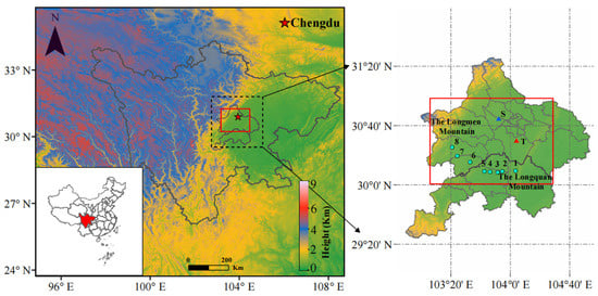
Figure 1.
Geographical distribution of UAV sounding sites along the SA3 highway. The UAV sounding sites, numbered from 1 to 8, are located along the SA3 highway and include Heilongtan (1), Funiu (2), Meishan North (3), Yuexing (4), Duoyue (5), Shou’an West (6), Kongming (7), and Datong (8). The blue triangle (S) represents the Wenjiang meteorological station, while the red triangle (T) denotes the in situ CO observation site.
Amid rapid urbanization and industrialization, Chengdu’s carbon emissions have become critical concerns. A study of the Chengdu metropolitan area revealed that economic development was the primary driver of carbon emissions, contributing to an increase of 23.80 million tons, while energy intensity emerged as the leading mitigation factor, reducing emissions by 11.07 million tons [31]. Additionally, Chengdu’s GDP surged from 588.95 billion Chinese Yuan (CNY) in 2010 to 1771.67 billion CNY in 2020, reflecting an average annual growth rate of 12.95% alongside significant improvements in the city’s industrial structure [32]. Given these dynamics, understanding the characteristics of carbon emissions in Chengdu is of significant practical importance, offering insights into addressing the environmental challenges associated with its rapid development.
2.2. Sampling Instrumentation and Flight Design
This study utilized a type M600 drone, manufactured by the DJI Technology Corporation (Shenzhen, China) equipped with a GHG analyzer, type LGR-ICOS GLA133, manufactured by ABB (Figure S1). The analyzer utilized off-axis integrated cavity output spectroscopy (OA-ICOS) technology, enabling the simultaneous, high-precision measurements of methane, CO2, and water vapor, with a sampling temporal resolution of 1 Hz and a measurement accuracy of 0.35 ppm for CO2. The sample gas inlet was positioned with a vertical offset of 40 cm from the center of the UAV’s rotor plane, considering that this location receives the least impact from the rotors [33,34,35]. The analyzer was designed to be operated within a temperature range of 5 °C to 45 °C. Consequently, this system effectively facilitates the acquisition of reliable vertical atmospheric CO2 profiles.
To ensure accurate estimation of anthropogenic CO2 emission rates, UAV flight trajectories were carefully planned to capture air masses transported along the prevailing downwind direction. Analysis on the wind frequency distribution based on hourly wind direction data from the Wenjiang meteorological monitoring station from July to September in 2016–2023 (Figure S2) revealed dominant north-northeasterly and northerly wind patterns. Accordingly, the sounding site was positioned to the south of the urban center, adjacent to the Third Ring Expressway (SA3; Figure 1), thereby aligning the sampling location with the primary transport pathway of locally emitted pollutants. The resulting CO2 concentration profiles reflect downwind enhancements and are thus well suited for cross-sectional flux-based quantification of emissions in the area west of the Longquan Mountain in Chengdu.
The UAV soundings were conducted on 23 September 2024, beginning at 5:36 a.m. at the Datong site (103.35° E, 30.42° N, at 525 m above sea level—m ASL hereafter), followed by 6:12 a.m. at the Kongming site (103.41° E, 30.33° N, 579 m ASL), 7:11 a.m. at the Shou’an West site (103.55° E, 30.26° N, 540 m ASL), 8:34 a.m. at the Duoyue site (103.71° E, 30.15° N, 516 m ASL), 8:55 a.m. at the Yuexing site (103.77° E, 30.15° N, 422 m ASL), 9:19 a.m. at the Meishan North site (103.86° E, 30.14° N, 402 m ASL), and 9:52 a.m. at the Funiu site (103.91° E, 30.15° N, 461 m ASL), and ending at 10:24 a.m. at the Heilongtan site (104.06° E, 30.16° N, 496 m ASL). Due to airspace restrictions, soundings were carried out below 300 m above ground level. It is important to note that the cloudy and lightly-raining weather conditions which occurred that morning were suitable for cross-section sampling, as the clouds delayed the development of the boundary layer throughout the morning, reducing the adverse effects of limited sounding height.
With a flight altitude limit of 300 m above ground level, UAV sampling was able to fully encompass the planetary boundary layer (PBL) during the observation period, ensuring the coverage of the vast majority of anthropogenic emissions in this area. As shown in Figure S3, the PBL height—derived from ERA5 reanalysis data—ranged from 91.08 m to 256.57 m during the sounding period, confirming that the observed profiles encompassed the key emission layer. Despite the occurrence of rainfall between 7:30 and 8:30 a.m., its impact on the estimation of emission rates was likely minimal. This was attributable to the light intensity and the short duration of the rainfall. Under such conditions, the rain exerted little influence on the CO2 concentrations according to a previous study [36].
2.3. Meteorological Parameters
Meteorological parameters, such as air temperature, pressure, and horizontal wind fields during the sampling period, were sourced from the ERA5 reanalysis dataset provided by the European Centre for Medium-Range Weather Forecasts (ECMWF). This dataset offers relevant variables with a spatial resolution of 0.25° × 0.25° every hour [37]. The air temperature, pressure, and u-/v-components of horizontal winds were vertically interpolated into the altitudes at which GHG concentrations were sampled.
To ensure the applicability of ERA5 data in this study, an accuracy assessment was conducted by comparing the ERA5 data from the grid cell corresponding to the Wenjiang meteorological station (103.870° E, 30.750° N) with the sounding data obtained at that station at 00:00 UTC on the sampling day. As shown in Figure 2, the parameters from the ERA5 dataset exhibit strong agreement with in situ measurements, with Pearson correlation coefficients (R) of 0.999, 0.722, 0.831, and 0.998 for air temperature, wind speed, wind direction, and pressure, respectively. All correlations were statistically significant (p < 0.01), indicating that the ERA5 data are reasonably accurate and statistically reliable for analyzing CO2 emission rates in UAV-based sounding measurements.
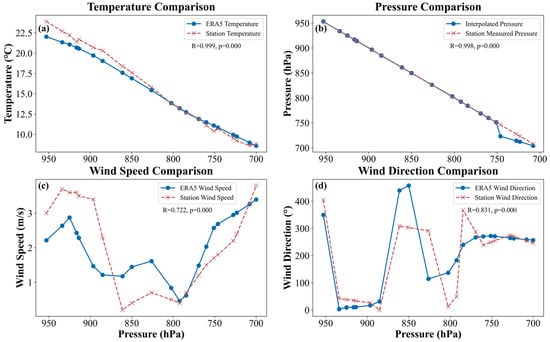
Figure 2.
Comparison of (a) temperature, (b) pressure, (c) wind speed, and (d) wind direction between the ERA5 dataset and sounding data at 00:00 on 23 September 2024, UTC. R and p represent the Pearson correlation coefficient and the p-value associated with the linear regression significance test, respectively.
2.4. UAV-Based Estimation of CO2 Emission Rates
2.4.1. Observation-Based Estimation of CO2 Emission Rates
The emission rates of CO2 were estimated by integrating CO2 concentration profiles and meteorological parameters, including temperature, wind speed, wind direction, and barometric pressure, thus employing the mass balance method. Firstly, the CO2 concentrations and meteorological parameters were interpolated to generate the cross-sectional distribution of these variables through a kriging interpolation method based on Gaussian modeling [24,38]. The resulting interpolated cross-sections achieved resolutions of 100 m and 5 m in the horizontal and vertical directions, respectively.
Based on these interpolated results, we delineated the background concentration areas to eliminate their influence on observed CO2 concentrations. Considering the mountain–plain–mountain terrain characteristics of Chengdu, anthropogenic CO2 is mainly emitted in the plain areas. The eastmost sounding site (Heilongtan) is a potential background site because it is located at the edge of the plain area and is far from any major emission sources as shown in Figure S4. By analyzing the observed profiles, we found that the concentrations at this site are relatively uniform and low. These characteristics align with typical background atmospheric conditions and effectively represent concentrations in areas far from local anthropogenic emission sources [10]. Thus, we chose the eastmost profile as the reference background concentrations for the entire cross-section.
For each grid cell in the cross-section, the anthropogenic CO2 flux was calculated using the CO2 enhancement, defined as the difference between the observed and background CO2 concentrations, as described in Equation (1).
where i represents the grid number; Fi is the anthropogenic CO2 flux in mol/(m2·s); Pi is the atmospheric pressure in Pa; is the wind component in the normal direction of the gird cell in m/s; E represents the CO2 enhancement in ppm; R is the gas constant; and Ti is the temperature in K [24].
The total anthropogenic CO2 emission rate in the upwind area of the cross-section was obtained by adding the fluxes of all grid cells [24,38], as depicted in Equation (2).
where ER denotes the emission rate in mol/s and Si is the area of the ith grid cell in m2.
2.4.2. Estimation of Yearly Emission Rates from the UAV-Based Emissions
Given that most existing emission inventories are reported on an annual basis, a meaningful evaluation of the UAV-based mass balance approach requires converting short-term flux measurements into annual estimates. Therefore, selecting an appropriate extrapolation strategy is essential to ensure comparability and assess the methodological reliability.
To address this challenge, we employed a proxy-based temporal scaling approach using fossil-fuel-derived CO2 (CO2,ff), inferred from ambient carbon monoxide (CO) concentrations. This method leverages the stable co-emission relationship between CO and CO2 during fossil fuel combustion and has been widely used to estimate anthropogenic emission strength under limited observational coverage. In this study, the CO2,ff-based scaling served as a physically grounded means to bridge the temporal gap between event-scale UAV observations and annual inventory data. By leveraging the proportional relationship between CO and CO2 emissions from fossil fuel combustion, CO2,ff was estimated using Equation (3).
where COxs represents the excess CO concentration, calculated as the difference between the observed CO concentration (COobs) and the background concentration (CObg), and R is the emission ratio of CO to CO2 during fossil fuel combustion, setting as R = 0.011 ± 0.002 [39]. In this study, COobs was obtained from the Tianfu New District air quality monitoring station in Chengdu, which is marked as site “T” in Figure 1. Hourly CO data from this site in 2023 were used for COxs calculation. The background concentration COobs was derived from monthly average CO values at Waliguan station (100°54′ E, 36°17′ N), a WMO/GAW global background site, which provides regionally representative conditions with minimal local emission influence (Table 1). Specifically, Figure S5 provides the long-term monthly mean CO concentrations at Waliguan from 1990 to 2023, from which the corresponding 2023 values were extracted for background correction in this study.

Table 1.
Monthly average CO and CO2 concentrations at the Mt. Waliguan station in 2023.
Given that UAV observations were conducted between 5:00 and 10:00 a.m. on 23 September, we employed the diurnal variation in CO2,ff concentrations during autumn to scale the observed morning fluxes to daily emissions. The scaling factor was defined as the ratio of the average CO2,ff concentration during the UAV sampling period to the full-day mean. To further extrapolate to the annual scale, seasonal scaling was applied based on the relative variation in CO2,ff across different seasons, thereby enabling the derivation of annual CO2 emissions from a single-day observation.
2.5. Census-Based Estimation of CO2 Emission Rates
To verify the effectiveness of UAV-based estimation of CO2 emissions, we utilized a bottom-up inventory approach to estimate the latter in Chengdu from 2010 to 2022, based on activity-level data from the Chengdu Statistical Yearbook. These census-based estimations were compared with UAV-based estimations to critically evaluate the validity of UAV sampling methods in GHG emission assessments.
We estimated Chengdu’s CO2 emissions by focusing on energy-related activities, primarily from the industrial, residential, and transportation sectors. Emissions from other sectors, such as agriculture and waste management, were excluded due to data limitations. This approach remains valid as energy activities account for the majority of urban CO2 emissions. According to the Carbon Emission Accounts and Datasets (CEADs), energy-related activities contributed about 80% of Chengdu’s total CO2 emissions, with the industrial and transportation sectors being the largest contributors [40,41,42].
CO2 emissions from energy-related activities in industrial and residential sectors were estimated using the inventory method, as outlined in Equation (4) [43].
where AD represents the fuel consumption amount in TJ (Table S2) and EF is the emission factor in tC/TJ.
CO2 emissions from the transportation sector were estimated by the reported vehicle populations and assumed annual mileages and fuel consumptions for vehicles using different fuels, including natural gas, gasoline, and diesel, as described in Equation (5) [44].
where Proad is the CO2 emission from transportation sector; Ni,k, li,k, and ei,k denotes the population, average annual mileage (km), and average fuel consumption per unit mileage (Nm3/100 km for natural gas and L/100 km for gasoline and diesel) of vehicles using fuel i in transportation mode k, including private cars, buses and taxis; and EFi is the emission factor for fuel i. As the population of diesel vehicles was not reported in the yearbook, we counted the number of diesel vehicles as 4.05% of the total vehicle population, in accordance with PAN Yu-jin et al. (2020) [45]. Taking the activity levels in 2022 as an example, Table 2 summarizes the number of vehicles and their corresponding annual mileages, and Table 3 provides energy consumption parameters, detailing the fuel consumption for each transportation mode. These values serve as key inputs in calculating fuel consumption and subsequent CO2 emissions. The carbon emission factors and energy conversion parameters for various fuel types are listed in Table S2 [43].
Table 2.
Activity levels of different vehicle types in 2022.
Table 3.
Fuel type and fuel consumption parameters.
3. Results
3.1. UAV Sounding Results
The observed CO2 profiles are presented in Figure 3, and the interpolated spatial distribution of CO2 concentrations covering the cross-section is presented in Figure S6. The vertical profiles obtained during UAV ascent and descent appeared broadly similar at all sounding sites, although notable differences in concentration values were observed at several locations, notably Datong (Site 8; Figure 3a), Yuexing (Site 4; Figure 3e), and Meishan North (Site 3; Figure 3f). These disparities are likely a result of airflow disturbances caused by UAV’s rotors. The higher levels of power required during the UAV’s ascent intensify the rotor disturbance, which leads to more dramatic fluctuations in the concentrations of ascension profiles, subsequently resulting in artificially elevated local pollutant concentrations and a decrease in the reliability of the profiles. Therefore, we selected the descending profiles for analysis.
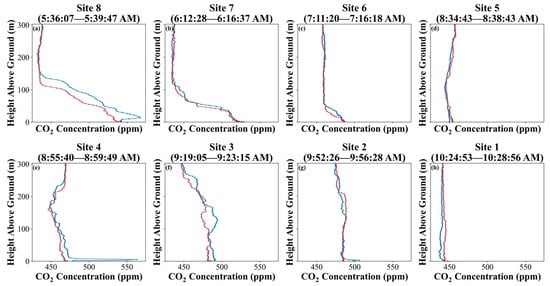
Figure 3.
CO2 profiles during ascension (blue lines) and descension (red lines) at (a) site 8, (b) site 7, (c) site 6, (d) site 5, (e) site 4, (f) site 3, (g) site 2, and (h) site 1.
The observed CO2 concentrations were higher near the surface (below 100 m) and gradually decreased with increasing altitude. This pattern aligns with the typical emission characteristics of urban areas, where ground-level emission sources—such as traffic, industrial activities, and residential emissions—lead to the accumulation of air pollutants near the surface. Spatially, Datong (Site 8; Figure 3a) and Kongming (Site 7; Figure 3b) exhibited pronounced near-surface CO2 enhancements, while Meishan North (Site 3; Figure 3f) and Funiu (Site 2; Figure 3g) displayed elevated concentrations throughout the entire observed column. This distribution pattern resulted from the combined effects of emission source distribution and boundary layer dynamics. The western sites are located near the regions of Qionglai and Dayi, which are known for dense industrial emission sources (Figure S4). During the sounding period, the planetary boundary layer height remained below the sampling height as illustrated in Figure S3. Under these conditions, the CO2 emitted from these sources tended to accumulate near the surface, resulting in the observed high concentrations. In contrast, the eastern sites are situated in downwind areas which are further from emission sources. Longer transmission distances result in a higher vertical diffusion range, which leads to the absence of significantly higher near-surface concentrations.
3.2. Emission Rate and Its Uncertainties
The anthropogenic CO2 fluxes penetrating the cross-section are shown in Figure 4, and the vertically integrated CO2 emission rates for each subsection are presented in Table 4. The spatial distribution of the anthropogenic CO2 flux across the observation region showed significant heterogeneity. Higher flux values were concentrated in the central and eastern subsections, likely driven by local anthropogenic sources such as industrial operations, vehicular traffic, and residential activities, compounded by the prevailing northern wind present during the observation period. In contrast, the western subsections exhibited relatively lower flux values, which could be attributed to the relatively calm winds (Figures S7–S12).
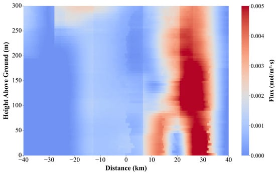
Figure 4.
Estimated anthropogenic CO2 fluxes crossing through the subsections. The horizontal axis represents the distance from the midpoint of the observation trajectory, with a negative value on the west side and a positive value on the east side.
Table 4.
Vertically integrated CO2 emission rates for each subsection.
The emission values in Table 4 were obtained by integrating emissions over individual grid cells (100 m horizontal × 5 m vertical resolution) shown in Figure 4. By summing the fluxes across all grid cells within each subsection, the total CO2 emission rate was determined as 35,398.62 mol/s during the observation period (5:00–10:00 a.m.), providing a quantitative assessment of anthropogenic carbon emissions during this timeframe.
The uncertainties of the estimated CO2 emission rate arise from multiple independent factors, including temperature, pressure, CO2 enhancement [49], and potential contributions from surrounding regions. Among these, the first three can be quantitatively assessed. To integrate their effects, the total uncertainty (δER) was calculated using the standard uncertainty propagation formula, which combines the relative contributions from each factor as follows:
where F is the coverage factor set to 2, corresponding to a 95% confidence level, following the convention of expanded uncertainty estimation in atmospheric studies [49].
The uncertainty in the estimated CO2 enhancement (δE/E) arises from two primary sources: the measurement uncertainty associated with observed CO2 concentrations and the uncertainty in the background concentration. Given that the instrumental precision for CO2 measurements has been previously specified, the uncertainty of the observed concentrations (ΔC) was set to 0.35 ppm. The uncertainty of the background concentration was represented by the standard deviation (σbg) of the background concentrations. The overall uncertainty in the CO2 enhancement is then computed as follows:
where Cobs and Cbg represent the mean observed and background concentrations, respectively.
The uncertainties of temperature and pressure were determined based on the differences between ERA5 reanalysis data and field sounding data, , where σdiff is the standard deviation of the differences and is the mean value of the corresponding physical quantity.
The total uncertainty results for temperature (δT/T = 4.73%), pressure (δP/P = 0.75%), and enhancement (δE/E = 10.79%) were propagated to estimate the overall uncertainty in emission rate (δER), which was calculated as 23.61% by applying the uncertainty propagation formula. The results indicate that the enhancement contributes the most to the overall uncertainty, while the impact of pressure uncertainty is relatively minor; it is important to emphasize that these represent the minimal or lower-bound uncertainty, as noted in prior studies [50]. Furthermore, the spatial and temporal resolution limitations of ERA5 (e.g., 0.25° and 1 h intervals) prevent the effective capture of real-time atmospheric variability, and thus limit synchronization with high-frequency CO2 measurements collected by UAV-borne analyzers. This introduces potential systematic biases beyond what is captured by the relative uncertainty calculation. Elevated ambient humidity following rainfall may introduce uncertainty due to potential cross-sensitivity between CO2 and H2O in the optical analyzer. While the ABB LGR-ICOS GLA133 incorporates automatic water vapor correction, its performance under high-humidity conditions remains unverified. Moreover, standard gas calibration was not consistently conducted prior to each flight. This potential bias, though unquantified, warrants consideration in future uncertainty assessments.
In addition to the quantifiable sources above, an unquantified uncertainty stems from potential cross-boundary air mass transport. To qualitatively assess this, 24 h back trajectory footprints at altitudes of 5 m to 300 m were analyzed. The results (Figures S13–S16) show that air masses at lower altitudes were primarily confined within Chengdu’s administrative boundary. However, at higher levels (200–300 m), minor contributions from neighboring regions, such as Deyang and Mianyang, were observed. Although these external influences were limited, their exact contribution to CO2 flux remains unquantified in this study. Future work should incorporate more refined trajectory modeling and regional source attribution techniques to better constrain such external impacts.
3.3. Comparison Between Census and UAV-Based Estimations of CO2 Emissions
3.3.1. Census-Based Emission Rates
This study utilized a bottom-up inventory approach to systematically estimate CO2 emissions in Chengdu from 2010 to 2022 employing the methods presented in Section 2.5 and based on the activity levels from the Chengdu Statistical Yearbook as summarized in Tables S3 and S4. Additionally, Table S5 provides a comprehensive record of vehicle ownership in Chengdu from 2010 to 2022, offering essential data for assessing emissions from the transportation sector. The calculated emissions were cross-validated against data from the CEADs for the same period to assess the reliability and applicability of the inventory method for regional carbon emission quantification.
The estimation results and the comparison with CEAD data are illustrated in Figure 5a. Census-based CO2 emissions showed a trend of steady growth, which closely aligned with the fluctuations in the CEADs records. This consistency demonstrated that the inventory method in this study was able to capture variations in urban GHG emissions. Chengdu’s CO2 emissions increased from approximately 3550 MtCO2 to 4220 × 104 tCO2e from 2010 to 2012 with an average annual growth rate of 6.0%. This increase was mainly driven by economic growth and rising energy consumption. However, from 2012 to 2015, emissions declined by approximately 11.8%, likely due to energy-saving policies and industrial upgrading. From 2015 onwards, emissions grew rapidly and reached 5330 × 104 tCO2e by 2019, reflecting the accelerated industrialization and urbanization of this city.
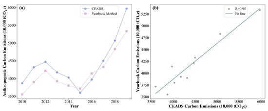
Figure 5.
Annual variations (a) and comparison between the emissions from CEADs [51,52,53,54] and this study (b).
A strong correlation was observed between the census-based emission and CEAD estimates during 2010–2019 (R = 0.95; Figure 5b), indicating good agreement in interannual variation. The discrepancies between the energy-related emissions estimated in this study and the CEAD data primarily stemmed from differences in emission source coverage. The census-based CO2 data reported in this study comprise energy-related emissions only, which count for about 90% of the emissions in the CEADs during the assessed period, except in 2015 and 2016. The average ratio between the estimated energy-related emissions in this study and the emissions in the CEAD dataset was 0.93. This ratio was then applied to estimate the total CO2 emissions from 2020 to 2022 based on the census-based energy related emissions. These total emissions were subsequently extrapolated linearly to project emissions in 2024, which were about 6929 × 104 tCO2e (69.29 MtCO2e). The emissions in the area west of the Longquan Mountain accounted for about 87.62% of the total emissions in Chengdu, according to the spatial distribution of CO2 emissions as presented in Figure S4. Therefore, the census-based CO2 emissions in the area west of the Longquan Mountain in Chengdu were estimated to be 60.71 MtCO2e.
3.3.2. Estimated Annual CO2 Emissions Based on UAV Observations
The variations in CO2,ff reflect the relative intensity of anthropogenic emissions. The diurnal variations in CO2,ff concentrations across different seasons are illustrated in Figure 6. Similar diurnal trends were observed in all seasons, with CO2,ff concentrations peaking during the late morning to early afternoon (approximately 9:00–15:00) and decreasing during the night [55]. This pattern reflects the daily cycle of human activities, such as traffic and industrial operations, which are more intense during the daytime. Additionally, lower boundary layer heights at night limit vertical diffusion, leading to the accumulation of emissions near the surface.
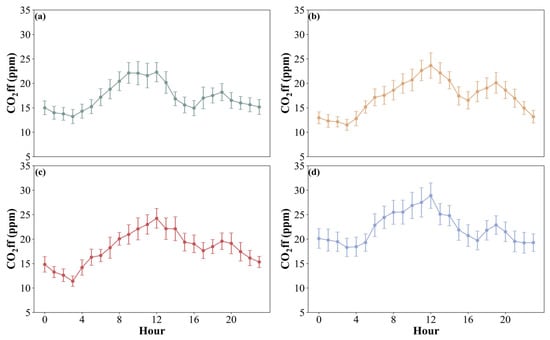
Figure 6.
Diurnal variations in CO2,ff concentrations during (a) spring, (b) summer, (c) autumn, and (d) winter. Error bars indicate the standard deviations of mean CO2,ff concentrations.
Despite the general similarity in diurnal profiles, notable seasonal differences in the magnitude of CO2,ff concentrations were observed. Winter saw the highest CO2,ff concentrations, with peak values approaching 30 ppm, ascribed to increased heating requirements and emissions from residential and industrial activities. In contrast, summer had lower concentrations, typically beneath 20 ppm during the night, owing to reduced heating emissions and a more evolved boundary layer facilitating pollutant dispersion. Spring and autumn exhibited intermediate levels of CO2,ff, mirroring the transitional character of energy utilization and meteorological conditions during these periods. These discoveries emphasize the combined impact of anthropogenic activities and seasonal meteorological dynamics on CO2,ff variations, highlighting its dependability as an indicator of emission intensity.
Because UAV observations were carried out from 5:00 to 10:00 a.m. on 23 September, we employed the diurnal variations in CO2,ff concentrations in autumn (Table S6) to estimate daily CO2 emissions based on the UAV recorded emission rate of 35,398.62 mol/s. The ratio between the average CO2,ff concentrations during the 5:00–10:00 a.m. period and the entire day is 0.262. Therefore, the daily CO2 emission should amount to 2.91 × 10⁹ mol (35,398.62 mol/s × 21,600 s/0.262). Similarly, by using the ratio of the averaged seasonal CO2,ff concentrations during autumn, as well as other seasons (Table S7), the annual CO2 emission was estimated as being approximately 1.10 × 10¹² mol (4.84 × 10⁷ tons CO2). The average annual UAV recorded annual CO2 emission was estimated as 48.40 Mt CO2, which was consistent in magnitude with the census-based estimation (60.71 MtCO2). This indicates the potential of UAV observations in the capturing of overall emissions.
This result aligns in magnitude with the census-based estimation (60.71 MtCO2), supporting the representativeness of the UAV-derived estimate despite its single-day origin. The extrapolation was not based on simple scaling but incorporated the observed diurnal and seasonal patterns of fossil-fuel-derived CO2 (CO2,ff), providing a physically informed correction for limited temporal coverage.
While uncertainties remain—mainly from the coarse resolution of ERA5 meteorological data and the fixed CO/CO2 emission ratio—the methodological consistency between UAV-based and inventory-based estimates demonstrates the feasibility of this approach for urban-scale emission assessments. The observational period was selected to reflect typical morning boundary layer dynamics and anthropogenic activity, enhancing temporal representativeness. Although continuous year-round UAV sampling is impractical, this study suggests that strategically timed measurements across different seasons can improve the robustness and generalizability of emission estimates. Future research should integrate higher-resolution meteorological inputs and multi-seasonal UAV deployments to further reduce uncertainty and extend the applicability of this cost-effective method to complex urban environments.
4. Discussion
This study demonstrates the potential of UAV-based mass balance methods as a flexible and cost-effective approach for estimating urban CO2 emissions. Through high-resolution vertical profiling at multiple sites, we successfully captured morning boundary layer CO2 enhancements and derived city-scale emission estimates. Compared to conventional aircraft or ground-based systems, UAV platforms offer greater spatial flexibility and can be deployed rapidly in urban environments. These advantages highlight their applicability in data-limited regions and for supplementing existing emission monitoring frameworks.
This study demonstrated that carefully designed UAV campaigns can provide meaningful snapshots of CO2 flux dynamics when aligned with boundary layer development. But in this preliminary trial, the measurements reflect only early morning conditions, which may not fully capture the diurnal emission cycle or the development of the afternoon boundary layer. This temporal limitation may reduce the representativeness of the derived fluxes. In future campaigns, UAV observations conducted across diverse seasons and various times of the day can be systematically integrated to more accurately characterize the temporal variability of urban CO2 emissions. These findings support the value of targeted UAV measurements in urban emission assessment.
One aspect not addressed in this study is the contribution of biospheric CO2 fluxes. Given Chengdu’s substantial urban vegetation, early-morning CO2 uptake may influence near-surface concentrations and partially offset anthropogenic signals. Future studies could incorporate biosphere–atmosphere exchange modeling or isotopic techniques (e.g., δ13C analysis) to help distinguish biogenic and fossil-fuel sources.
Meteorological inputs—particularly wind speed and direction—remain a key source of uncertainty in flux calculations. This study used ERA5 reanalysis data, which may not resolve complex urban wind fields. Previous studies have shown that wind estimates can also be derived from UAV flight dynamics [56] or directly measuring winds using UAV-mounted ultrasonic anemometers [57]. Incorporating such methods, or coupling UAV data with high-resolution urban meteorological models, would help refine future analyses. In particular, replacing coarse-resolution reanalysis datasets such as ERA5 with mesoscale numerical weather prediction outputs (e.g., WRF at about 1 km resolution) can substantially reduce flux estimation uncertainties arising from misrepresented wind structures. Also, technological advancements are expected to improve the utility of this method. With increased payload capacity and sensor miniaturization, future UAVs may carry onboard meteorological modules (e.g., ultrasonic anemometers or LiDAR), enabling real-time wind field characterization and reducing uncertainties. Enhanced endurance and battery life would further enable extended vertical and temporal coverage, potentially capturing full boundary layer development across the day.
Various approaches have been proposed to scale short-term emission measurements to annual estimates, often tailored to specific source types and data availability. For instance, point-source emissions have been extrapolated using detailed operational records, while high-frequency monitoring networks in urban areas have enabled representative flux patterns through temporal aggregation [15,23]. UAV-based measurements have also been applied at event scale, though such applications typically require extended and repeated sampling to ensure temporal representativeness [58]. However, these strategies are not directly applicable to this study due to observational constraints such as limited flight durations, meteorological dependencies, and the absence of sector-specific operational data.
To address this, we adopted a CO2,ff-based scaling method using ambient CO as a tracer for fossil fuel emissions. This approach normalizes UAV-derived fluxes based on the diurnal and seasonal variability of CO2,ff, enabling extrapolation to annual scales. The effectiveness of this method relies on the choice of background station, the accuracy of the CO:CO2 emission ratio (R), and the stability of the tracer relationship across emission types. In our case, due to the limited availability of localized CO and CO2 datasets in Chengdu, a literature-derived R value was adopted based on similar urban contexts. We acknowledge that this substitution introduces uncertainty, as R values may vary across combustion sources and cities. This limitation underscores the need for localized characterization of R through targeted observations, which will be considered in future work. Although our estimate showed reasonable agreement with inventory data, this serves as an initial consistency check rather than formal validation. Future work could benefit from integrating isotopic constraints or inverse modeling to further evaluate the reliability of this proxy-based extrapolation. Nonetheless, this method offers a practical solution for bridging the temporal gap between short-term UAV observations and inventory-scale emission assessments in data-limited environments. In summary, while limitations exist, this study confirms the feasibility of using UAV-based mass balance methods for urban CO2 emission assessments. With further methodological refinements, this approach shows strong potential to support near-source monitoring, inventory validation, and policy-relevant carbon accounting in urban areas. Although the UAV-derived annual emissions showed general agreement with inventory data, the 23.61% deviation is non-negligible and should be interpreted as an approximate constraint. Nevertheless, if this deviation remains stable over time, the UAV-based method could still be valuable for tracking emission trends, offering a promising tool for assessing long-term changes driven by policy or socioeconomic factors.
5. Conclusions
The feasibility of applying UAV-based mass balance methods for urban CO2 emission estimation has been effectively demonstrated through an integrated framework combining vertical UAV soundings with ERA5 meteorological data. This approach offers a flexible and cost-efficient alternative to conventional monitoring techniques, particularly in urban areas where high-resolution, near-surface observations are essential. In the Chengdu case study, the CO2 emission rate derived from UAV observations was approximately 35,398.62 mol/s, yielding an annual emission estimate of 48.40 MtCO2. Although this estimate showed general consistency with the census-based value of 60.71 MtCO2, the relative deviation of 23.61% is non-negligible and reflects the inherent uncertainties of using short-term data. This uncertainty is primarily attributed to the accuracy and spatial-temporal resolution of meteorological inputs such as CO2 enhancements, temperature, and pressure.
While these limitations constrain the robustness of absolute emission estimation, the method demonstrates promise as a complementary tool for near-source monitoring and emission inventory evaluation. With extended temporal coverage—through multi-period observations across seasons—and continued methodological improvements, this UAV-based approach may also offer potential for tracking interannual emission trends, which is particularly relevant for climate change mitigation efforts in urban areas.
Supplementary Materials
The following supporting information can be downloaded at: https://www.mdpi.com/article/10.3390/atmos16060713/s1, Figure S1: Sampling system of UAV type DJI M600 Pro equipped with greenhouse gas analyzer type ABB LGR-ICOS GLA133; Figure S2: Wind rose chart of Chengdu during July to September in 2016–2023; Figure S3: The planetary boundary layer heights of Chengdu during the sounding period; Figure S4. Spatial Distribution of (a) annual emissions and (b) emissions in September in 2017; Figure S5: Monthly trends of CO2 and CO concentrations at Waliguan station from 1990 to 2023; Figure S6: Kriging interpolation results showing the distribution of CO2 concentrations; Figure S7: Wind field distributions over Chengdu at 975 hPa (a), 950 hPa (b), 925 hPa (c), and 900 hPa (d) at 5:00 a.m. on September 23, with the black outline indicating the administrative boundary of Chengdu; Figure S8: Wind field distributions over Chengdu at 975 hPa (a), 950 hPa (b), 925 hPa (c), and 900 hPa (d) at 6:00 a.m. on September 23, with the black outline indicating the administrative boundary of Chengdu. Figure S9: Wind field distributions over Chengdu at 975 hPa (a), 950 hPa (b), 925 hPa (c), and 900 hPa (d) at 7:00 a.m. on September 23, with the black outline indicating the administrative boundary of Chengdu; Figure S10: Wind field distributions over Chengdu at 975 hPa (a), 950 hPa (b), 925 hPa (c), and 900 hPa (d) at 8:00 a.m. on September 23, with the black outline indicating the administrative boundary of Chengdu; Figure S11. Wind field distributions over Chengdu at 975 hPa (a), 950 hPa (b), 925 hPa (c), and 900 hPa (d) at 9:00 a.m. on 23 September, with the black outline indicating the administrative boundary of Chengdu; Figure S12. Wind field distributions over Chengdu at 975 hPa (a), 950 hPa (b), 925 hPa (c), and 900 hPa (d) at 10:00 a.m. on September 23, with the black outline indicating the administrative boundary of Chengdu; Figure S13: Spatial distribution of normalized 24 h footprints at 5 m above ground level (normalized by maximum residence time); Figure S14: Spatial distribution of normalized 24 h footprints at 100 m above ground level (normalized by maximum residence time); Figure S15: Spatial distribution of normalized 24 h footprints at 200 m above ground level (normalized by maximum residence time); Figure S16: Spatial distribution of normalized 24 h footprints at 300 m above ground level (normalized by maximum residence time); Table S1. Summary of data information used in this study; Table S2. Carbon Emission Conversion Factors for Fossil Fuels; Table S3. Energy activity levels from the industrial sector in Chengdu, as reported in the Chengdu Statistical Yearbook from 2010 to 2022; Table S4. Energy activity levels from the residential sector in Chengdu, as reported in the Chengdu Statistical Yearbook from 2010 to 2022; Table S5. Vehicle Ownership by Type in Chengdu from 2010 to 2022; Table S6. Hourly CO2,ff concentrations in autumn; Table S7. Seasonal averaged CO2,ff concentrations.
Author Contributions
Conceptualization, G.S. and K.X.; methodology, X.X. and G.S.; validation, X.X.; investigation, X.X., K.X., X.W. (Xing Wang), X.W. (Xi Wang), X.K., X.Z. and L.Z.; resources, K.X., X.W. (Xing Wang) and X.W. (Xi Wang); data curation, X.X. and X.K.; writing—original draft preparation, X.X.; writing—review and editing, G.S. and F.Y.; supervision, F.Y. All authors have read and agreed to the published version of the manuscript.
Funding
This research was funded by the National Key R&D Program of China, grant number 2023YFC3709301; the National Natural Science Foundation of China, grant number 42175124; and the Fundamental Research Funds for the Central Universities, China, grant number 2023CDSN-18.
Institutional Review Board Statement
Not applicable.
Informed Consent Statement
Not applicable.
Data Availability Statement
The original contributions presented in this study are included in the article/supplementary material. Further inquiries can be directed to the corresponding author.
Conflicts of Interest
The authors declare no conflicts of interest.
References
- Liu, X.; Xu, H.Z.; Zhang, M. The effects of urban expansion on carbon emissions: Based on the spatial interaction and transmission mechanism. J. Clean. Prod. 2024, 434, 140019. [Google Scholar] [CrossRef]
- Sitompul, M.; Suroso, A.I.; Sumarwan, U.; Zulbainarni, N. Revisiting the Impact of Corporate Carbon Management Strategies on Corporate Financial Performance: A Systematic Literature Review. Economies 2023, 11, 171. [Google Scholar] [CrossRef]
- C40 Cities. The Low Carbon Investment Landscape in C40 Cities: An Analysis of the Sustainable Infrastructure Projects Currently in Development Across C40 Cities. Available online: https://www.c40.org/researches/the-low-carbon-investment-landscape-in-c40-cities (accessed on 6 February 2025).
- Wu, T.; An, M.Q.; Zhang, L.L.; Wu, X.Z.; Li, M.Y. Modeling urban expansion and its impacts on carbon storage through integrative scenario analysis for sustainable development in the Changchun-Jilin-Tumen region. Sustain. Cities Soc. 2024, 117, 105970. [Google Scholar] [CrossRef]
- Hu, Q.L.; Mijit, R.; Xu, J.X.; Miao, S. Can government-led urban expansion simultaneously alleviate pollution and carbon emissions? Staggered difference-in-differences evidence from Chinese firms. Econ. Anal. Policy 2024, 84, 1–25. [Google Scholar] [CrossRef]
- Xiao-Yi, L.I.; Rui, W.U. Research on greenhouse gas emissions accounting boundaries and calculating method of the transport sector. Adv. Clim. Change Res. 2023, 19, 84–90. [Google Scholar]
- Oda, T.; Bun, R.; Kinakh, V.; Topylko, P.; Halushchak, M.; Marland, G.; Lauvaux, T.; Jonas, M.; Maksyutov, S.; Nahorski, Z.; et al. Errors and uncertainties in a gridded carbon dioxide emissions inventory. Mitig. Adapt. Strateg. Glob. Change 2019, 24, 1007–1050. [Google Scholar] [CrossRef]
- Andres, R.J.; Boden, T.A.; Bréon, F.M.; Ciais, P.; Davis, S.; Erickson, D.; Gregg, J.S.; Jacobson, A.; Marland, G.; Miller, J.; et al. A synthesis of carbon dioxide emissions from fossil-fuel combustion. Biogeosciences 2012, 9, 1845–1871. [Google Scholar] [CrossRef]
- Boden, T.A.; Marland, G.; Andres, R.J. Global, Regional, and National Fossil-Fuel CO2 Emissions (1751–2014) (V. 2017). 1999. Available online: https://data.ess-dive.lbl.gov/view/doi:10.3334/CDIAC/00001_V2017 (accessed on 10 March 2025).
- Oda, T.; Maksyutov, S.; Andres, R.J. The Open-source Data Inventory for Anthropogenic CO2, version 2016 (ODIAC2016): A global monthly fossil fuel CO2 gridded emissions data product for tracer transport simulations and surface flux inversions. Earth Syst. Sci. Data 2018, 10, 87–107. [Google Scholar] [CrossRef] [PubMed]
- Bo, X.; Shan, W.Y.; Qu, J.B.; Lei, T.T.; Sang, M.J.; Li, Z.L.; Lin, A.J. Construction of a high-resolution city-level emission inventory based on multiple methods: A case study of Cangzhou City, China. Environ. Dev. Sustain. 2025. [Google Scholar] [CrossRef]
- Xia, L.; Liu, R.; Fan, W.X.; Ren, C.X. Emerging carbon dioxide hotspots in East Asia identified by a top-down inventory. Commun. Earth Environ. 2025, 6, 10. [Google Scholar] [CrossRef]
- Huang, W.J.; Griffis, T.J.; Hu, C.; Xiao, W.; Lee, X.H. Seasonal Variations of CH4 Emissions in the Yangtze River Delta Region of China Are Driven by Agricultural Activities. Adv. Atmos. Sci. 2021, 38, 1537–1551. [Google Scholar] [CrossRef]
- Hu, C.; Xu, J.P.; Liu, C.; Chen, Y.; Yang, D.; Huang, W.J.; Deng, L.C.; Liu, S.D.; Griffis, T.J.; Lee, X.H. Anthropogenic and natural controls on atmospheric δ13C-CO2 variations in the Yangtze River delta: Insights from a carbon isotope modeling framework. Atmos. Meas. Tech. 2021, 21, 10015–10037. [Google Scholar] [CrossRef]
- Liggio, J.; Li, S.M.; Staebler, R.M.; Hayden, K.; Darlington, A.; Mittermeier, R.L.; O’Brien, J.; McLaren, R.; Wolde, M.; Worthy, D.; et al. Measured Canadian oil sands CO2 emissions are higher than estimates made using internationally recommended methods. Nat. Commun. 2019, 10, 1863. [Google Scholar] [CrossRef]
- Cui, X.; Newman, S.; Xu, X.; Andrews, A.E.; Miller, J.; Lehman, S.; Jeong, S.; Zhang, J.; Priest, C.; Campos-Pineda, M.; et al. Atmospheric observation-based estimation of fossil fuel CO2 emissions from regions of central and southern California. Sci. Total Environ. 2019, 664, 381–391. [Google Scholar] [CrossRef] [PubMed]
- Zhong, W.Y.; Zhai, D.S.; Xu, W.R.; Gong, W.W.; Yan, C.; Zhang, Y.; Qi, L.Y. Accurate and efficient daily carbon emission forecasting based on improved ARIMA. Appl. Energ. 2024, 376, 124232. [Google Scholar] [CrossRef]
- Liu, H.L.; Hu, C.; Xiao, Q.T.; Zhang, J.Q.; Sun, F.; Shi, X.J.; Chen, X.; Yang, Y.R.; Xiao, W. Analysis of anthropogenic CO2 emission uncertainty and influencing factors at city scale in Yangtze River Delta region: One of the world’s largest emission hotspots. Atmos. Pollut. Res. 2024, 15, 102281. [Google Scholar] [CrossRef]
- Mallia, D.V.; Mitchell, L.E.; Vidal, A.E.G.; Wu, D.; Kunik, L.; Lin, J.C. Can We Detect Urban-Scale CO2 Emission Changes Within Medium-Sized Cities? J. Geophys. Res.-Atmos. 2023, 128, e2023JD038686. [Google Scholar] [CrossRef]
- Mays, K.L.; Shepson, P.B.; Stirm, B.H.; Karion, A.; Sweeney, C.; Gurney, K.R. Aircraft-Based Measurements of the Carbon Footprint of Indianapolis. Environ. Sci. Technol. 2009, 43, 7816–7823. [Google Scholar] [CrossRef]
- Cambaliza, M.O.L.; Shepson, P.B.; Caulton, D.R.; Stirm, B.; Samarov, D.; Gurney, K.R.; Turnbull, J.; Davis, K.J.; Possolo, A.; Karion, A.; et al. Assessment of uncertainties of an aircraft-based mass balance approach for quantifying urban greenhouse gas emissions. Atmos. Chem. Phys. 2014, 14, 9029–9050. [Google Scholar] [CrossRef]
- Zhang, S.Q.; Lei, L.P.; Sheng, M.Y.; Song, H.; Li, L.M.; Guo, K.Y.; Ma, C.H.; Liu, L.Y.; Zeng, Z.C. Evaluating Anthropogenic CO2 Bottom-Up Emission Inventories Using Satellite Observations from GOSAT and OCO-2. Remote Sens. 2022, 14, 5024. [Google Scholar] [CrossRef]
- Turner, A.J.; Shusterman, A.A.; McDonald, B.C.; Teige, V.; Harley, R.A.; Cohen, R.C. Network design for quantifying urban CO2 emissions: Assessing trade-offs between precision and network density. Atmos. Chem. Phys. 2016, 16, 13465–13475. [Google Scholar] [CrossRef]
- Cambaliza, M.O.L.; Shepson, P.B.; Bogner, J.; Caulton, D.R.; Stirm, B.; Sweeney, C.; Montzka, S.A.; Gurney, K.R.; Spokas, K.; Salmon, O.E.; et al. Quantification and source apportionment of the methane emission flux from the city of Indianapolis. Elementa Sci. Anthr. 2015, 3, 000037. [Google Scholar] [CrossRef]
- Mohsan, S.A.H.; Othman, N.Q.H.; Li, Y.L.; Alsharif, M.H.; Khan, M.A. Unmanned aerial vehicles (UAVs): Practical aspects, applications, open challenges, security issues, and future trends. Intell. Serv. Robot. 2023, 16, 109–137. [Google Scholar] [CrossRef]
- Wong, G.; Wang, H.; Park, M.; Park, J.; Ahn, J.-Y.; Sung, M.; Choi, J.; Park, T.; Ban, J.; Kang, S.; et al. Optimizing an airborne mass-balance methodology for accurate emission rate quantification of industrial facilities: A case study of industrial facilities in South Korea. Sci. Total Environ. 2024, 912, 169204. [Google Scholar] [CrossRef] [PubMed]
- Khaleghi, A.; MacKay, K.; Darlington, A.; James, L.A.; Risk, D. Methane emission rate estimates of offshore oil platforms in Newfoundland and Labrador, Canada. Elementa Sci. Anthrop. 2024, 12, 00025. [Google Scholar] [CrossRef]
- Han, T.R.; Liggio, J.; Narayan, J.; Liu, Y.Y.; Hayden, K.; Mittermeier, R.; Darlington, A.; Wheeler, M.; Cober, S.; Zhang, Y.H.; et al. Quantification of Methane Emissions from Cold Heavy Oil Production with Sand Extraction in Alberta and Saskatchewan, Canada. Environ. Sci. Technol. 2024, 58, 13284–13295. [Google Scholar] [CrossRef]
- Han, T.; Xie, C.; Liu, Y.; Yang, Y.; Zhang, Y.; Huang, Y.; Gao, X.; Zhang, X.; Bao, F.; Li, S.M. Development of a continuous UAV-mounted air sampler and application to the quantification of CO2 and CH4 emissions from a major coking plant. Atmos. Meas. Tech. 2024, 17, 677–691. [Google Scholar] [CrossRef]
- Tomlin, J.M.; Lopez-Coto, I.; Hajny, K.D.; Pitt, J.R.; Kaeser, R.; Stirm, B.H.; Jayarathne, T.; Floerchinger, C.R.; Commane, R.; Shepson, P.B. Spatial attribution of aircraft mass balance experiment CO2 estimations for policy-relevant boundaries: New York City. Elementa Sci. Anthrop. 2023, 11, 00046. [Google Scholar] [CrossRef]
- Yu, J.; Yu, L.; Luo, Y.N.; Zhang, P.W. Research on the development path of Chengdu as a low-carbon city under the dual constraints of carbon emission and economic growth. Front. Environ. Sci. 2024, 12, 1494848. [Google Scholar] [CrossRef]
- Xu, M.; Yang, X.; Deng, L.L.; Liao, X.; Niu, Z.S.; Hao, L.N. Decoupling state of urban development and carbon emissions and its driving factors and predictions: A case study of Chengdu metropolitan area. Ecol. Inform. 2024, 82, 102692. [Google Scholar] [CrossRef]
- Leitner, S.; Feichtinger, W.; Mayer, S.; Mayer, F.; Krompetz, D.; Hood-Nowotny, R.; Watzinger, A. UAV-based sampling systems to analyse greenhouse gases and volatile organic compounds encompassing compound-specific stable isotope analysis. Atmos. Meas. Tech. 2023, 16, 513–527. [Google Scholar] [CrossRef]
- Do, S.; Lee, M.; Kim, J.S. The Effect of a Flow Field on Chemical Detection Performance of Quadrotor Drone. Sensors 2020, 20, 3262. [Google Scholar] [CrossRef]
- Zhou, S.D.; Peng, S.L.; Wang, M.; Shen, A.; Liu, Z.H. The Characteristics and Contributing Factors of Air Pollution in Nanjing: A Case Study Based on an Unmanned Aerial Vehicle Experiment and Multiple Datasets. Atmosphere 2018, 9, 343. [Google Scholar] [CrossRef]
- Liu, C.J.; Ilvesiemi, H.; Kutsch, W.; Ma, X.Q.; Westman, C.J.; Kauppi, P. An estimate on the rainout of atmospheric CO2. J. Environ. Sci. 2004, 16, 86–89. [Google Scholar]
- Hersbach, H.; Bell, B.; Berrisford, P.; Biavati, G.; Horányi, A.; Muñoz Sabater, J.; Nicolas, J.; Peubey, C.; Radu, R.; Rozum, I.; et al. ERA5 Hourly Data on Pressure Levels from 1940 to Present; Copernicus Climate Change Service (C3S): Reading, UK, 2023; Climate Data Store (CDS). [Google Scholar] [CrossRef]
- Holzworth, G.C. Mixing Depths, Wind Speeds and Air Pollution Potential for Selected Locations in the United States. J. Appl. Meteorol. Climatol. 1967, 6, 1039–1044. [Google Scholar] [CrossRef]
- Wunch, D.; Wennberg, P.O.; Toon, G.C.; Keppel-Aleks, G.; Yavin, Y.G. Emissions of greenhouse gases from a North American megacity. Geophys. Res. Lett. 2009, 36, 15810. [Google Scholar] [CrossRef]
- Shan, Y.L.; Huang, Q.; Guan, D.B.; Hubacek, K. China CO2 emission accounts 2016–2017. Sci. Data 2020, 7, 54. [Google Scholar] [CrossRef]
- Shan, Y.L.; Guan, D.B.; Zheng, H.R.; Ou, J.M.; Li, Y.; Meng, J.; Mi, Z.F.; Liu, Z.; Zhang, Q. Data Descriptor: China CO2 emission accounts 1997–2015. Sci. Data 2018, 5, 170201. [Google Scholar] [CrossRef] [PubMed]
- Xu, J.H.; Guan, Y.R.; Oldfield, J.; Guan, D.B.; Shan, Y.L. China carbon emission accounts 2020–2021. Appl. Energ. 2024, 360, 122837. [Google Scholar] [CrossRef]
- IPCC. 2019 Refinement to the 2006 IPCC Guidelines for National Greenhouse Gas Inventories; IPCC: Geneva, Switzerland, 2019. Available online: https://www.ipcc.ch/report/2019-refinement-to-the-2006-ipcc-guidelines-for-national-greenhouse-gas-inventories/ (accessed on 6 February 2025).
- Tian, P.-N.; Mao, B.-H.; Tong, R.-Y.; Zhang, H.-X.; Zhou, Q. Analysis of carbon emission level and intensity of China’s transportation industry and different transportation modes. Adv. Clim. Change Res. 2023, 19, 347–356. [Google Scholar]
- Pan, Y.J.; Li, Y.; Chen, J.H.; Shi, J.C.; Tian, H.; Zhang, J.; Zhou, J.; Chen, X.; Liu, Z.; Qian, J. Method for High-resolution Emission Inventory for Road Vehicles in Chengdu Based on Traffic Flow Monitoring Data. Huan Jing Ke Xue 2020, 41, 3581–3590. [Google Scholar] [PubMed]
- Ministry of Industry and Information Technology of the People’s Republic of China. Announcement of Average Fuel Consumption and New Energy Vehicle Credits of Chinese Passenger Vehicle Enterprises for 2019. Available online: https://ythxxfb.miit.gov.cn/ythzxfwpt/hlwmh/zcwj/xzxk/clsczr/art/2020/art_a14a402f2b5b4ac6addad2998f845fd0.html (accessed on 6 February 2025).
- National Energy Administration. Economical and Environmentally Friendly Natural Gas Buses Operating in Many Parts of Jiangxi Province. Available online: http://www.nea.gov.cn/2012-10/19/c_131915953.htm (accessed on 6 February 2025).
- Gao, J.; Xiao, Y.; Wang, J. Research on Emission and Energy Consumption Evaluation Method of National VI Heavy-Duty Diesel Vehicles. Sci. Dev. Res. 2022, 2, 82–85. [Google Scholar]
- Heimburger, A.; Losno, R.; Triquet, S.; Nguyen, E.B. Atmospheric deposition fluxes of 26 elements over the Southern Indian Ocean: Time series on Kerguelen and Crozet Islands. Glob. Biogeochem. Cycles 2013, 27, 440–449. [Google Scholar] [CrossRef]
- Heimburger, A.; Harvey, R.; Shepson, P.; Stirm, B.; Gore, C.; Turnbull, J.; Cambaliza, M.; Salmon, O.; Kerlo, A.-E.; Lavoie, T.; et al. Assessing the optimized precision of the aircraft mass balance method for measurement of urban greenhouse gas emission rates through averaging. Elem. Sci. Anth. 2017, 5, 26. [Google Scholar] [CrossRef]
- Shan, Y.L.; Guan, Y.R.; Hang, Y.; Zheng, H.R.; Li, Y.X.; Guan, D.B.; Li, J.S.; Zhou, Y.; Li, L.; Hubacek, K. City-level emission peak and drivers in China. Sci. Bull. 2022, 67, 1910–1920. [Google Scholar] [CrossRef]
- Shan, Y.L.; Guan, D.B.; Hubacek, K.; Zheng, B.; Davis, S.J.; Jia, L.C.; Liu, J.H.; Liu, Z.; Fromer, N.; Mi, Z.F.; et al. City-level climate change mitigation in China. Sci. Adv. 2018, 4, eaaq0390. [Google Scholar] [CrossRef]
- Shan, Y.L.; Guan, D.B.; Liu, J.H.; Mi, Z.F.; Liu, Z.; Liu, J.R.; Schroeder, H.; Cai, B.F.; Chen, Y.; Shao, S.; et al. Methodology and applications of city level CO2 emission accounts in China. J. Clean. Prod. 2017, 161, 1215–1225. [Google Scholar] [CrossRef]
- Shan, Y.L.; Liu, J.H.; Liu, Z.; Shao, S.; Guan, D.B. An emissions-socioeconomic inventory of Chinese cities. Sci. Data 2019, 6, 190027. [Google Scholar] [CrossRef]
- Vogel, F.R.; Hammer, S.; Steinhof, A.; Kromer, B.; Levin, I. Implication of weekly and diurnal 14C calibration on hourly estimates of CO-based fossil fuel CO2 at a moderately polluted site in southwestern Germany. Tellus B. Chem. Phys. Meteorol. 2010, 62, 512–520. [Google Scholar] [CrossRef]
- Zhao, T.H.; Yang, D.X.; Guo, D.; Wang, Y.; Yao, L.; Ren, X.Y.; Fan, M.; Cai, Z.N.; Wu, K.; Liu, Y. Low-cost UAV coordinated carbon observation network: Carbon dioxide measurement with multiple UAVs. Atmos. Environ. 2024, 332, 120609. [Google Scholar] [CrossRef]
- Kim, K.T.; Kim, H.; Jeong, S.; Lee, Y.S.; Choi, E.; Kim, J.Y. Quantification of greenhouse gas emissions from a municipal solid waste incinerator using an uncrewed aerial vehicle. Environ. Int. 2025, 198, 109396. [Google Scholar] [CrossRef] [PubMed]
- Shah, A.; Ricketts, H.; Pitt, J.R.; Shaw, J.T.; Kabbabe, K.; Leen, J.B.; Allen, G. Unmanned aerial vehicle observations of cold venting from exploratory hydraulic fracturing in the United Kingdom. Environ. Res. Commun. 2020, 2, 021003. [Google Scholar] [CrossRef]
Disclaimer/Publisher’s Note: The statements, opinions and data contained in all publications are solely those of the individual author(s) and contributor(s) and not of MDPI and/or the editor(s). MDPI and/or the editor(s) disclaim responsibility for any injury to people or property resulting from any ideas, methods, instructions or products referred to in the content. |
© 2025 by the authors. Licensee MDPI, Basel, Switzerland. This article is an open access article distributed under the terms and conditions of the Creative Commons Attribution (CC BY) license (https://creativecommons.org/licenses/by/4.0/).