Article

Assessment of Aromatic Hydrocarbons in Urban Air: A Study from a Northern Mexican Megacity

by
Julia Griselda Cerón Bretón
1,
Rosa María Cerón Bretón
1,*,
Claudia Alejandra Aguilar Ucán
1,
Carlos Montalvo Romero
1,
Alberto Antonio Espinosa Guzmán
2,
Simón Eduardo Carranco Lozada
3,
Evangelina Ramírez Lara
4,
María de la Luz Espinosa Fuentes
5 and
Martha Patricia Uc Chi
1
1
Facultad de Química, Universidad Autónoma del Carmen, Ciudad del Carmen 24180, Mexico
2
Centro de Investigación en Corrosión, Universidad Autónoma de Campeche, San Francisco de Campeche 24079, Mexico
3
CECyT 15, Instituto Politécnico Nacional, Ciudad de México 12100, Mexico
4
Facultad de Ciencias Químicas, Universidad Autónoma de Nuevo León, San Nicolas de Los Garza 66455, Mexico
5
Instituto de Ciencias de la Atmósfera y Cambio Climático, Universidad Nacional Autónoma de México, Ciudad de Mexico 04510, Mexico
*
Author to whom correspondence should be addressed.
Atmosphere 2025, 16(6), 649; https://doi.org/10.3390/atmos16060649
Submission received: 14 March 2025 / Revised: 17 May 2025 / Accepted: 23 May 2025 / Published: 27 May 2025
(This article belongs to the Special Issue Air Quality in Metropolitan Areas and Megacities (Second Edition))

Abstract

The spatiotemporal distributions of aromatic hydrocarbon levels in the atmosphere were evaluated at ten locations within Monterrey’s Metropolitan Area using passive sampling techniques across three climatic seasons (the rainy season of 2023, the cold front season of 2023, and the dry season of 2024). The observed relative abundance was toluene > p-xylene > benzene > ethylbenzene. The dry season showed the highest concentration values for all measured compounds, and the Santa Catarina site showed the highest average level for toluene (2.79 μg m−3). In the rainy season, the highest average concentrations were recorded in Santa Catarina, with toluene at 1.39 μg m−3 and p-xylene at 0.99 μg m−3. During the cold fronts season, the greatest average concentration of p-xylene (0.98 μg m−3) was found in San Bernabe, while Santa Catarina reported the highest average for toluene at 1.55 μg m−3. A health risk assessment indicated that cancer risk coefficients exceeded the reference values set by the EPA. These findings suggest that the presence of the alkyl derivatives of benzene (benzene, toluene, ethylbenzene, and p-xylene) in the studied region poses a potential health issue and highlights the need for enhanced control measures regarding their sources.

1. Introduction

Urban populations are continuously exposed to a complex mixture of air pollutants, many of which pose significant health risks. Among these, toxic air contaminants such as volatile organic compounds (VOCs) have garnered increasing attention in indoor and outdoor environments due to their association with respiratory, cardiovascular, and carcinogenic effects [1]. A particularly concerning subset of VOCs is BTEX—which includes benzene, toluene, ethylbenzene, and xylenes. These compounds play a crucial role in atmospheric chemistry as precursors for secondary air pollutants such as tropospheric ozone, fine particulate matter (PM2.5), and other photochemical oxidants [2]. Their ability to undergo photochemical reactions contributes to urban smog formation, exacerbating air quality deterioration in highly populated areas [3].
The United States Environmental Protection Agency (EPA) classifies BTEX as Hazardous Air Pollutants (HAPs) due to their acute and chronic health effects [4]. Among them, benzene is of particular concern, as it has been designated as a Group 1 carcinogen by the International Agency for Research on Cancer (IARC), meaning there is sufficient evidence linking its exposure to leukemia and other hematologic disorders [5]. The prolonged inhalation of BTEX compounds is also associated with neurological impairments, liver and kidney dysfunction, and developmental toxicity, making their presence in the ambient air a significant public health issue.
BTEX are emitted from a variety of anthropogenic sources, including vehicular traffic, industrial operations, fuel storage and distribution facilities, surface coatings, and solvent applications. In urban environments, on-road and non-road gasoline-powered vehicles are among the primary contributors [6], particularly in regions with high vehicle density and inadequate emissions regulations. Consequently, continuous air quality monitoring is essential to understanding BTEX distribution, assessing human exposure risks, and informing regulatory policies aimed at reducing harmful emissions in urban areas.
One such region of concern is the Metropolitan Area of Monterrey (MAM), the second-largest metropolitan area in Mexico and one of the most industrially and economically active regions in the country. According to a study by the National Institute of Ecology and Climate Change [7], vehicular emissions in the MAM generate 40% more carbon monoxide (CO) and five times higher hydrocarbon (HC) emissions than those reported in Mexico City. Furthermore, an estimated 70% of vehicles in the MAM are over ten years old, indicating a prevalence of outdated engines with limited or no emissions control systems. As of 2025, the total number of vehicles in circulation within the MAM, including private and public transport, is projected to reach approximately 1,835,711 [8]. These factors contribute significantly to air quality deterioration and potential aromatic hydrocarbons accumulation in the region.
The MAM operates an air quality monitoring network consisting of 13 well-functioning stations; however, these stations do not measure the levels of benzene and its alkyl derivatives (benzene, toluene, ethylbenzene, and p-xylene). It is imperative to evaluate the concentrations of these compounds in ambient air across various urban areas within the MAM, as well as to ascertain the health risks associated with exposure for the affected population.
In large urban environments, air pollution levels can vary significantly due to high vehicular emissions, industrial activities, and population density. In such contexts, passive devices are an excellent choice for monitoring air pollutants [9]. In this study, we selected passive samplers to measure benzene, toluene, ethylbenzene, and p-xylene because they are cost-effective, easy to use, and suitable for long-term exposure assessments. Passive sampling techniques offer several advantages over active sampling, especially for large-scale environmental monitoring [10,11]. Unlike active sampling, which requires pumps and electrical power, passive samplers use molecular diffusion to collect air pollutants over time. Various studies have effectively employed Radiello passive samplers to measure BTEX in different settings. For example, Cocheo et al. [9] utilized Radiello samplers to assess BTEX concentrations in urban and industrial areas across Europe, demonstrating their efficacy for long-term air quality monitoring. Additionally, Chaiklieng et al. (2021) [12] used Radiello samplers to evaluate BTEX exposure among gasoline station workers, confirming their relevance in occupational health studies. Furthermore, Cruz et al. [13] deployed passive samplers in high-traffic areas, showing that the Radiello samplers accurately reflect the patterns of vehicular emissions.
Consequently, this research aims to (a) examine seasonal variations in the atmospheric concentrations of benzene and its alkyl derivatives (toluene, ethylbenzene, and p-xylene) throughout three climatic seasons at ten designated locations within the MAM, employing passive sampling devices, (b) identify the areas within the MAM that exhibit the highest concentrations for these compounds, and (c) assess the risks associated with these compounds through inhalation, taking into account both carcinogenic and non-carcinogenic effects, including the potential for the development of respiratory and cardiovascular diseases. In addition, this study will provide essential data that will drive evidence-based policy recommendations, enhance air quality management strategies, and strengthen public health protections in one of Mexico’s most densely populated urban centers.

2. Materials and Methods
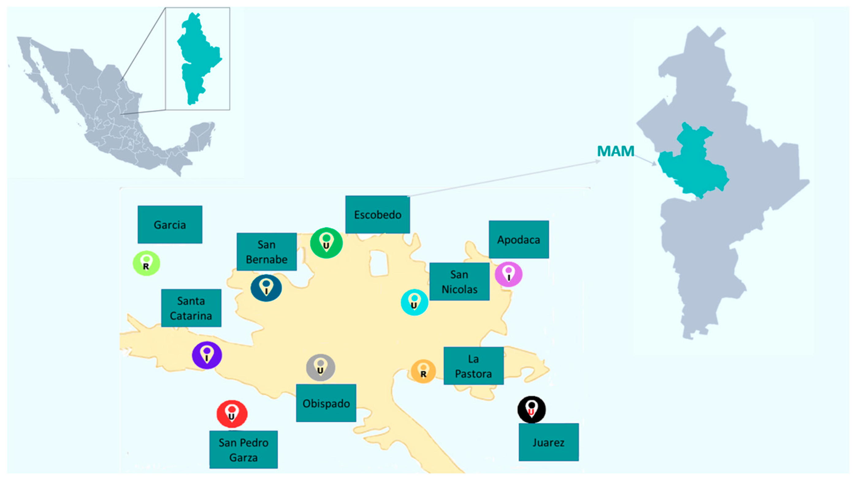
2.1. Study Area

The MAM is situated in the state of Nuevo Leon in northern Mexico. A total of ten sampling locations were chosen, each representing various types of land use: industrial, urban, and rural. These locations include Obispado, Escobedo, San Bernabe, Garcia, San Nicolas, Apodaca, Santa Catarina, San Pedro Garza, La Pastora, and Juarez (Figure 1).
The selection of sampling sites was based on several criteria, such as physical conditions, access, safety, electrical supply, and representativeness. In 2019, the National Institute of Statistics, Geography, and Informatics [7], along with the National Council of Population [14], identified the MAM as a region made up of 18 municipalities, housing a total of 4,689,601 residents across an area of 7657 km2, with a growth rate of 2.2% between 2010 and 2015, and an average urban density of 108.3 inhabitants per hectare [7,14].
The sampling points are located within the air quality monitoring stations managed by the Environmental Monitoring Integrated System (SIMA) of the Government of the State of Nuevo Leon, ensuring spatial consistency and data comparability with routine atmospheric monitoring protocols. These monitoring stations track key air pollutants (O3, CO, NO2, SO2, PM10, and PM2.5) along with meteorological data.

2.2. Sampling Method

Sampling was conducted using Radiello™ diffusive passive samplers installed in 10 different sites. These passive samplers are characterized by providing higher capacity and faster sampling rates than traditional passive samplers [15,16]. Diffusion cartridges of Sigma Aldrich ™ (St. Louis, MO, USA) model Radiello cartridge adsorbents of 60 mm length and 5.8 mm in diameter were used. Cartridges were built of stainless steel (100 mesh; 5.8 mm diameter), and packed with activated carbon (30–50 mesh). These devices were placed inside a polyethylene container (diffuser body) of 60 mm height × 16 mm diameter, in which there is a diffusion membrane of a 25 µm pore size, which allows the controlled diffusion of pollutant gases toward the adsorbent tube, at a diffusion rate of 80 mL min−1 [17,18,19]. The sampling period spanned 24 weeks, with 8 weeks designated for each climatic season (the rainy season of 2023, the cold front season of 2023, and the dry season of 2024) and was organized into 2-week intervals during which the sampling tubes were exposed for two weeks, being collected at the end of this period. Sampling for the 2023 rainy season began on 26 June 2023 and concluded on 20 August 2023. During the cold front season, samples were collected from 16 October to 4 December 2023. For the dry season, sampling took place between 4 March and 28 April 2024. A total of 120 samples were collected from 10 different sampling sites, with 40 samples collected for each climatic season. Immediately following the sampling, the sorbent tubes were sealed with end caps to ensure the integrity of the samples. Subsequently, these tubes were stored in airtight glass amber vials to safeguard the samples from environmental exposure and to prevent the photodegradation of the measured compounds. The vials were maintained in a padded cooler under cool and dark conditions to minimize the evaporation of volatile compounds and to mitigate the risk of photodegradation. Upon arrival in the laboratory, the samples were stored at a refrigeration temperature of 4 °C. An analysis of the samples was conducted within 48 h of collection to ensure the accuracy of the measurements.
After sampling, the analytes retained on the sorbent were desorbed by chemical extraction with 1 mL of Carbon Disulfide (CS2), and extracts were stored in amber vials of 2 mL with a threaded cap and septa. Subsequently, extracts were subjected to an ultrasonic bath for 10 min at 10 °C [13,17], stored under refrigeration, and analyzed by using a standard GC/FID instrument within a maximum of 72 h after desorption.

2.3. Sampling Quality Control/Quality Assurance (QA/QC)

Field blanks (additional Sigma Aldrich™ (St. Louis, MO, USA) model Radiello diffusive samplers) were included to assess contamination from handling or transportation and were set at the same conditions as the actual samples and analyzed using the same procedures. Duplicate samples were obtained for each sampling site (replicates) in each sampling period throughout the 14-day exposure period to assess precision and they were prepared and analyzed identically. The results were adjusted according to the blank values.
During the analysis, before starting the sampling, an equipment blank (empty sorbent tube) was run through the system to check for any contamination. Standard and QC samples were analyzed alongside field samples to ensure that the analytical system was functioning correctly. This process was carried out as part of the Sampling Quality Control/Quality Assurance (QA/QC) program.

2.4. Analysis Method

The samples were analyzed using the sampling and analysis method MTA/MA-030/A92 from the National Institute of Safety and Hygiene of Spain [17]. A Gas Chromatograph (TRACE GC Ultra Thermo Fisher Scientific Technologies, Inc., Waltham, MA, USA) coupled to a flame ionization detector (Thermo Fisher Scientific Technologies, Inc., Waltham, MA, USA) was used in a splitless mode to analyze the collected samples. The analytical conditions were as follows: (a) A fused silica methyl-type capillary column (30 m × 0.32 mm ID, with a film thickness of 0.5 µm, stationary phase: 5%-Phenyl-methylpolysiloxane) was used. (b) The oven temperature program was set to 40 °C for 4 min, and then the temperature was increased at a rate of 5 °C min−1 up to 100 °C and maintained for 10 min. (c) Ultra-pure nitrogen (99.999%) was used as the carrier gas at 1 mL min−1. (d) The flame ionization detector (FID) used ultra-pure hydrogen and extra-dried air at 35 mL min−1 and 350 mL min−1, respectively.
Table 1 outlines the method detection limits (MDLs), accuracy, precision, and linearity for the analytical method employed to quantify the measured aromatic hydrocarbons using gas chromatography with flame ionization detection (GC-FID) [20]. A seven-point calibration was conducted at concentrations of 0.05, 0.10, 1.00, 5.00, 15.00, 50.00, and 100.00 µg mL−1, utilizing 99.98% pure Sigma Aldrich™ analytical reagents (Sigma Aldrich Inc., St. Luois, MO, USA) for each compound. The limits of detection (LODs) were 0.05, 0.06, 0.06, and 0.05 µg mL−1 for benzene, toluene, ethylbenzene, and p-xylene, respectively. The corresponding R-squared values from this calibration are presented in Table 1.
The method detection limits (MDLs) were determined by calculating the standard deviation from seven replicate measurements at a concentration of 0.0.05 µg/mL and multiplying this by 1.943, based on the t-distribution for n = 7 at a 95% confidence level. The relative standard deviation (% RSD) was evaluated for each compound. Accuracy was assessed through repeated measurements of the solutions of the compounds of interest across the 0.10 to 100.00 µg mL−1 concentration range, with the results documented in Table 2. Detection limits are considered acceptable when the coefficient of variation remains below 10% for all measured compounds. It can be observed in Table 1 that the analytical method is both accurate and precise within the tested range. Linearity is regarded as acceptable when R2 values exceed 0.995, supported by a p-value in the ANOVA of less than 0.001.

2.5. Estimation of Aromatic Hydrocarbon Ratios

Aromatic hydrocarbon ratios consist of obtaining the quotient between toluene and benzene (T/B) and between p-xylene and ethylbenzene (X/E) and are used to identify the relative importance of the sources of these compounds during a given period. These ratios are useful to determine if the emissions are coming from mobile or area sources (T/B ratio) or the degree of aging of air masses (X/E ratio). Benzene and toluene are the main constituents of gasoline, and for this reason, T/B ratios are used as indicators of vehicular traffic. T/B ratio values between 2 and 3 suggest that vehicular emissions contributed significantly to the measured pollutants. T/B values greater than 3 mean that the measured compound levels can be associated with industrial sources or area sources such as evaporative, automotive paint, coking, and more [21]. The X/E ratio is used to identify the age of air masses in a given location [22,23]. Low values of this ratio indicate fresh air masses from recent emissions, while high values indicate aged emissions. Values for this ratio between 3.8 and 4.4 have been reported in sites influenced by fresh gasoline emissions [22].

2.6. Meteorological Analysis and Measurement of Criteria Air Pollutants

Meteorological variables (wind speed, wind direction, ambient temperature, relative humidity, solar radiation, atmospheric pressure, and precipitation) and criteria air pollutant concentrations (O3, CO, SO2, NO2, PM10, and PM2.5) were obtained from SIMA (Integrated System of Environmental Monitoring of Nuevo Leon State) for both study periods. Surface meteorology was assessed by using wind roses obtained from WRPLOT View v. 8.0.2 [24], and backward trajectories were built using the HYSPLIT Model [25] to track air masses to assess the transport and dispersion of pollutants in the study sites.

2.7. Statistical Analysis

The Friedman test was applied to investigate significant differences in BTEX concentrations across the different sampling sites and climatic seasons. This non-parametric statistical method is effective for detecting differences in treatments among multiple related groups. It is especially applicable when the assumptions of normality and the homogeneity of variances, required by repeated measures ANOVA, are not satisfied [26]. In this analysis, the Spearman correlations between the measured aromatic hydrocarbons (benzene, toluene, ethylbenzene, and p-xylene), air pollutants (CO, NO2, O3, PM10, PM2.5, SO2), and meteorological factors during the three climatic seasons were obtained to provide insights into pollution sources, atmospheric interactions, and potential health implications. Spearman’s rank correlation coefficient (ρ\rhoρ) is a non-parametric statistical measure that assesses the strength and direction of monotonic relationships between two variables [27,28]. Unlike the Pearson correlation, Spearman correlation does not assume a linear relationship and is more robust against non-normal data distributions common in air pollution studies.

2.8. Health Risk Assessment Method

The European Union recommends a limit of 5 μg m−3 for benzene in ambient air, with a minimal risk level (MRL) of cancer by inhalation of 1 in 10,000. On the other hand, the US EPA establishes a value of 9 μg m−3 for this pollutant [29]. In this research work, we used the methodology proposed by Zhang et al. [30] to determine the daily exposure (Exp), the lifetime risk of cancer (RCLT), and the potential of non-cancer risk (HzQ). The daily exposure of an individual was calculated as follows:
E x p = C o n c × I R a p × D e x p M B W
Here, Exp represents the daily exposure to benzene in milligrams per kilogram of body weight per day, Conc is the mean concentration of benzene in milligrams per cubic meter, IRap is the inhalation rate for an adult person (0.83 cubic meters per hour) [31], Dexp is the duration of the exposure for an adult person (24 h per day), and MBW is the mean body weight for an adult (65 kg).
The risk of developing cancer due to benzene exposure over a lifetime was calculated according to
R C L T = E x p × S L F
Here, RCLT is the risk of cancer in the lifetime; SLF is the risk slope factor by inhalation of toxics (2.98 × 10⁻² kg day mg−1), which means that the carcinogenic effects by exposure can be considered linear. A value for SLF of 2.98 × 10⁻² kg day mg−1 for benzene was considered according to the US EPA [31]. On the other hand, non-cancer risk was estimated as the risk quotient, and was calculated as follows:
H z Q = C o n c R f C
Here, HzQ is the non-cancer risk for benzene; Conc is the daily dose received as annual mean in mg m−3; RfC is the reference concentration of inhalation in mg m−3. Specific values of RfC (mg m−3) have been proposed for each pollutant [32]: 0.03 for benzene, 5.0 for toluene, 1.0 for ethylbenzene, and 0.1 for p-xylene. The obtained values of non-cancer risk (HzQ) and cancer risk (RCLT) are compared with the limit values established by the US EPA [32].

3. Results

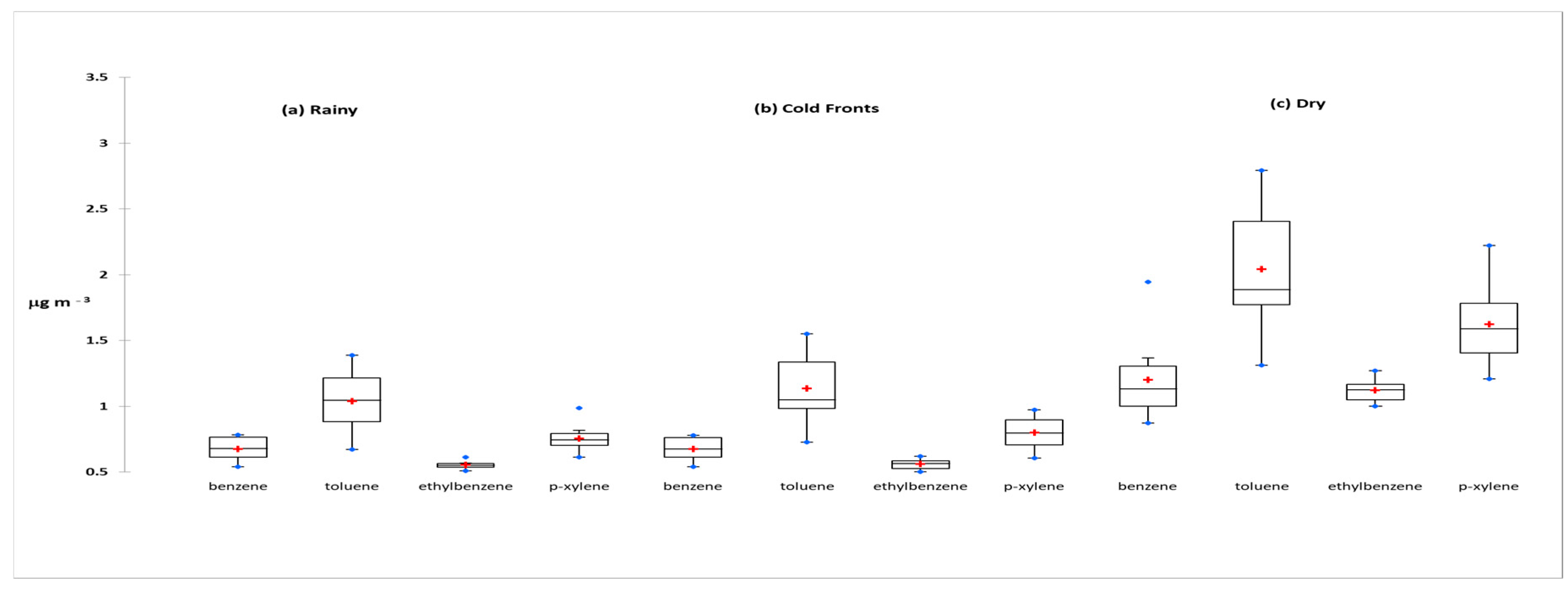
3.1. Seasonal Variation in Aromatic Hydrocarbon Concentrations

The relative abundance of the measured compounds was as follows: toluene (1.41 ± 0.30 µg m−3) > p-xylene (1.06 ± 0.15 µg m−3) > benzene (0.85 ± 0.16 µg m−3) > ethylbenzene (0.75 ± 0.10 µg m−3). Significant differences among these compounds were observed according to the Friedman test, with a significance level of alpha = 0.005, suggesting that the distribution of these compounds is influenced by various environmental and anthropogenic factors. Toluene’s predominance may be attributed to its widespread use in industrial and commercial applications, including solvents, gasoline additives, and coatings. Additionally, vehicular emissions and fuel evaporation are known to contribute significantly to atmospheric toluene levels. The presence of p-xylene and ethylbenzene in lower concentrations aligns with their typical emission sources, which include fuel combustion and industrial activities. Benzene, despite its high volatility and hazardous nature, was present at lower concentrations than toluene and p-xylene, possibly due to more stringent regulations on its use and emissions.
Figure 2 presents the descriptive statistics of the measured pollutant concentrations during three climatic seasons: the rainy season of 2023, the cold front season of 2023, and the dry season of 2024. All measured compounds exhibited the highest mean concentration values during the dry season, while lower mean concentrations were recorded during the cold fronts season, and the lowest levels were seen during the rainy season. Toluene, ethylbenzene, and p-xylene displayed significant differences in their concentrations across the different climatic seasons based on the Friedman test. Conversely, benzene did not show significant differences in concentration when comparing the rainy season with the cold fronts season.
During the rainy season, toluene had the highest average concentration (1.04 ± 0.26 µg m3), followed by p-xylene (0.75 ± 0.13 µg m3) and benzene (0.67 ± 0.09 µg m3), while ethylbenzene (0.55 ± 0.12 µg m3) had the lowest average concentration. The relative abundance of the measured compounds during the cold front season was toluene (1.13 ± 0.24 µg m3) > p-xylene (0.80 ± 0.09 µg m3) > benzene (0.68 ± 0.10 µg m3) > ethylbenzene (0.56 ± 0.08 µg m3), whereas the dry season showed the following relative abundance: toluene (2.04 ± 0.40 µg m3) > p-xylene (1.63 ± 0.24 µg m3) > benzene (1.20 ± 0.16 µg m3) > ethylbenzene (1.12 ± 0.11 µg m3).
The significantly higher levels of benzene, toluene, ethylbenzene, and p-xylene during the dry season can be attributed to meteorological conditions that promote the accumulation of pollutants. In this period, lower wind speeds and atmospheric stability limit the dispersion of pollutants [33]. Even though higher solar radiation and temperatures create conditions favorable for photochemical activity, aromatic hydrocarbons may not degrade efficiently if atmospheric mixing is limited due to stable layers or low winds or if the strength of the emissions sources is significant. Furthermore, the lower precipitation rates during the dry season reduce wet deposition [34], allowing the accumulation of these compounds in the air.
Conversely, the lowest concentrations were recorded during the rainy season. This is likely due to increased precipitation, which enhances the scavenging of pollutants through wet deposition. Higher humidity levels can influence the solubility and removal of these compounds from the air, and improved atmospheric mixing promotes the dispersion and dilution of these pollutants [35]. During the cold fronts season, intermediate levels were observed, reflecting the influence of stronger winds and temperature inversions. This behavior can be explained since during the rainy season, precipitation events promote the washout process along the atmospheric column, subsequently reducing the air pollutant concentrations at ground level [33]. It is important to highlight that in the MAM, since this is a zone with a semi-arid climate, the rains associated with the rainy season are considerably heavier in comparison with the rains associated with the cold fronts season, when only drizzles occur. This fact could explain why the dilution effect was more evident during the rainy season.

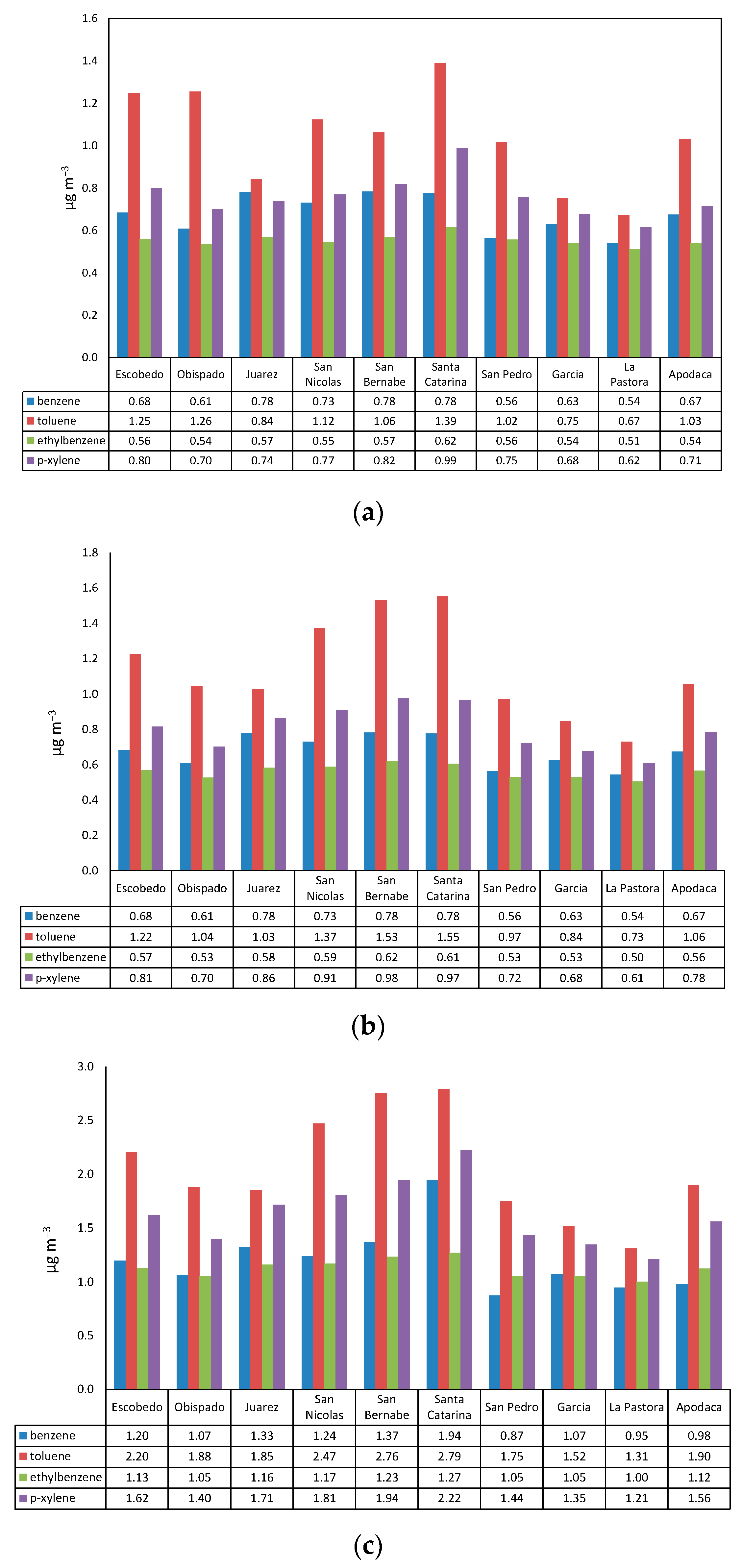
3.2. Aromatic Hydrocarbon Concentration Variations by Sampling Sites

In Figure 3a, the variability in the concentration of the measured pollutants by sampling sites during the rainy season can be observed, highlighting that the sites with the highest mean concentrations of benzene were San Bernabe with 0.78 μg m−3, Santa Catarina with 0.78 μg m−3, and Juarez with 0.78 μg m−3. The highest mean levels of toluene were found in Santa Catarina (1.39 μg m−3), Obispado (1.26 μg m−3), and Escobedo (1.25 μg m−3). The highest mean levels of ethylbenzene were found in Santa Catarina (0.62 μg m−3), followed by San Bernabe (0.57 μg m−3) and Escobedo (0.56 μg m−3). Finally, the highest concentrations of p-xylene were found in Santa Catarina (0.99 μg m−3), San Bernabe (0.82 μg m−3), and Escobedo (0.80 μg m−3).
Aromatic hydrocarbon concentrations obtained by the sampling site during the cold fronts season are shown in Figure 3b. The highest concentration of benzene was observed in San Bernabe (0.78 μg m−3), Santa Catarina (0.78 μg m−3), and Juarez (0.78 μg m−3). In the case of toluene, the highest levels were found in Santa Catarina with 1.55 μg m−3, San Bernabe with 1.53 μg m−3, and San Nicolas with 1.38 μg m−3. On the other hand, ethylbenzene showed its highest concentrations in San Bernabe with 0.62 μg m−3, followed by Santa Catarina with 0.61 μg m−3 and San Nicolas with 0.59 μg m−3. Finally, the highest values for p-xylene were obtained in San Bernabe with 0.98 μg m−3, Santa Catarina with 0.97 μg m−3, and San Nicolas with 0.91 μg m−3.
Figure 3c displays the concentrations of the measured compounds at various sampling sites during the dry season. Benzene concentrations were highest in Santa Catarina (1.94 μg m−3) and San Bernabe (1.37 μg m−3). Toluene showed elevated levels in Santa Catarina (2.79 μg m−3), San Bernabe (2.76 μg m−3), and San Nicolas (2.47 μg m−3). Additionally, ethylbenzene and p-xylene reached their peak concentrations in Santa Catarina and San Bernabe, measuring 1.27 μg m−3 and 1.23 μg m−3 for ethylbenzene and 2.22 μg m−3 and 1.94 μg m−3 for p-xylene, respectively. During all climatic seasons, the sites showing the lowest concentrations of BTEX were La Pastora and Garcia. This behavior was expected since they are rural sites.
The results reveal significant spatial variability in the concentrations of the measured compounds across different sampling sites in the Metropolitan Area of Monterrey (MAM). Notably, higher BTEX concentrations were consistently observed in Santa Catarina, San Bernabe, and San Nicolas, while lower concentrations were recorded in La Pastora and Garcia across all climatic seasons.
The elevated aromatic hydrocarbon levels in Santa Catarina, San Bernabe, and San Nicolas can be linked to the presence of major industrial activities (asphalt, cement, glass, chemical products, paintings, food, and so on), heavy vehicular traffic, and dense urban development. According to the socio-demographic profile of the MAM reported in the Population and Housing Census [36], these areas contain fuel storage facilities, manufacturing plants, and a high density of road vehicles, all of which contribute significantly to BTEX emissions [37,38]. Additionally, the prevalence of older vehicles in Monterrey [39] further exacerbates the emissions of these compounds due to inefficient combustion processes and inadequate emission control systems [40]. This situation is partly due to the proximity to the U.S. border, which results in a higher circulation of used vehicles that are older and less efficient.
San Bernabe is located in an area with a high population density to the west of an industrial zone characterized by heavy vehicular traffic.
In the case of Santa Catarina, there are 13 industrial parks, which feature major roadways like Avenida Morones Prieto and the Monterrey–Saltillo and Monterrey–Apodaca highways. Additionally, Santa Catarina is one of the main municipalities in the Metropolitan Area of Monterrey (MAM), representing approximately 7.1% of the total population in the MAM. For this reason, this area also experiences significant population mobility to and from other municipalities (the motorization rate for Santa Catarina is 345 vehicles per 1000 inhabitants). Santa Catarina’s orography could play an important role since this site is surrounded by hills (Mitras, La Silla, Las Escobas, Topo Chico, Las Tres Cruces, and Las Cuatro Piedras); in addition, most industries of the MAM are located in this zone [41].
San Nicolas, on the other hand, has experienced considerable business expansion in recent years, with retail and commerce being the primary activities, contributing 12.6% to the economy of the MAM. This municipality also has a robust industrial sector that produces metal products, machinery, transportation equipment, chemicals, plastics, construction materials, and food. In addition, San Nicolas has a high population density and faces significant mobility challenges, resulting in heavy vehicular traffic and increased emissions of volatile organic compounds (VOCs). These factors could contribute to elevated levels of aromatic hydrocarbons in the area.
In contrast, the rural areas of La Pastora and Garcia, characterized by lower traffic density, fewer industrial activities, and more vegetation, consistently exhibit lower levels of these compounds. This aligns with previous studies indicating that aromatic hydrocarbon concentrations are substantially lower in suburban and rural regions, where anthropogenic sources are reduced, and pollutant dispersion is greater [42].

3.3. Bivariate Analysis

The Spearman correlation matrix for the rainy season is shown in Table 2a, and it can be observed that the measured compounds have significant positive correlations among each other, suggesting that these compounds had their origin in common sources. Benzene showed a moderate positive correlation with SO2, suggesting that these compounds could have originated from common sources. It is worth noting that SO2 is often used as a tracer for industrial and vehicular emissions, particularly from diesel-powered vehicles. Benzene and SO2 may have common sources, such as industrial combustion sources that use fuels containing high levels of sulfur, as well as diesel vehicles. SO2 showed a significant negative correlation with ozone (−0.49). This can be explained due to SO2 being a substance that can lead to the formation of ozone in the atmosphere, since it reacts with nitrogen oxides in the presence of sunlight (these compounds are often released into the air by the burning of fossil fuels, industrial activities, and other anthropogenic activities) and form ozone in the troposphere [43]. Sulfur dioxide can also contribute to the formation of ozone through the production of particles that act as surfaces on which chemical reactions occur that generate ozone [44]. Toluene showed a significant negative correlation with ozone (−0.53), indicating that this compound could act as an ozone precursor in the study area. The oxidation reaction of toluene occurs via OH addition, forming organic peroxy radicals, converting NO to NO2 in an efficient way, and producing tropospheric ozone by the photolysis of NO2 [45]. Ethylbenzene and CO showed a negative correlation between each other (−0.58). Ethylbenzene is a chemical commonly used as an additive in gasoline to improve fuel quality and boost octane. It acts as an anti-knock agent, which helps prevent premature detonation in the engine, resulting in better engine efficiency and performance. Ethylbenzene can react with other compounds present in the atmosphere and produce carbon monoxide through oxidation; therefore, when it is released into the atmosphere, it can act as a precursor to carbon monoxide, explaining this negative correlation. In the presence of atmospheric oxygen, ethylbenzene can undergo oxidation by free radicals, such as hydroxyl radicals (·OH) or peroxyl radicals (RO·), which are produced from the decomposition of atmospheric pollutants like nitrogen oxides (NOx) or volatile organic compounds (VOCs). The process of oxidation involves breaking the carbon–hydrogen bonds of ethylbenzene, which results in the formation of alkyl radicals. These radicals can then react with oxygen to produce CO and other byproducts [46].
Table 2b presents the Spearman correlation matrix between aromatic hydrocarbons and criteria air pollutants during the cold fronts season. Statistically significant positive correlations were observed among benzene and its alkyl derivatives (toluene, ethylbenzene, and xylene), suggesting that these compounds likely originate from shared emission sources.
A strong negative correlation between O3 and PM10 (−0.68) was found. High concentrations of particulate matter in the atmosphere may attenuate solar radiation, limiting photochemical activity and, consequently, reducing ozone formation. These processes illustrate the complex, bidirectional interactions between O3 and PM10 under varying atmospheric conditions [47].
A significant negative correlation was also found between NO2 and PM2.5 (−0.72), which could indicate that under oxidizing atmospheric conditions, such as those observed during the MAM season (with elevated O3 and decreased NO2), the conversion of NO2 to nitric acid and other compounds promotes the formation of fine secondary aerosols.
Ozone and SO2 were positively correlated (0.72), a pattern reported in other studies [48]. However, this relationship is influenced by multiple factors, including gas-phase reactions involving NO2, water vapor, and photochemical activity, as well as variability in SO2 emission sources. Due to these overlapping influences, the interpretation of this correlation should be approached with caution.
PM10 and SO2 were negatively correlated (−0.69). While this may suggest a potential role for SO2 in sulfate aerosol formation through photochemical reactions, leading to its incorporation into particulate matter, as observed by Wilson et al. [49], other factors such as emission source variability and atmospheric dispersion should also be considered.
Benzene, ethylbenzene, and p-xylene showed moderate negative correlations with CO (−0.51, −0.48, and −0.45, respectively). These relationships could be attributed to differing formation and transformation pathways. For instance, CO is primarily produced through incomplete combustion, while BTEX compounds are also subject to atmospheric degradation through reactions with hydroxyl radicals (·OH), which, under specific conditions, may lead to CO formation as a byproduct [18,46].
Table 2c displays the correlations for the dry season. Strong positive correlations were found between benzene and toluene (0.75), benzene and ethylbenzene (0.86), and ethylbenzene and p-xylene (0.99), reinforcing the idea of common emission sources such as vehicular traffic, industrial processes, and fuel evaporation [37,50,51]. The very high correlation between ethylbenzene and p-xylene further suggests similarity in atmospheric behavior and degradation kinetics.
BTEX compounds also showed moderate positive correlations with NO2 (ranging from 0.47 to 0.53), which is consistent with their co-emission from combustion-related activities, including vehicle exhaust. In contrast, CO displayed weak or negative correlations with BTEX (from −0.15 to 0.04), highlighting potential differences in emission profiles. While CO is a marker of incomplete combustion, BTEX may be more associated with fuel-related evaporation and solvent use [52].
A moderate correlation between NO2 and O3 (0.30) indicates a partial influence of NO2 on ozone formation, although VOC concentrations, solar radiation, and meteorological conditions also play key roles [45,53]. Toluene’s stronger correlation with ozone (0.56) suggests a more direct involvement in photochemical ozone production via VOC oxidation.
Particulate matter (PM10 and PM2.5) showed mostly weak or negative correlations with BTEX compounds, supporting the idea that aerosol formation during this season is likely driven by regional or secondary processes rather than direct emissions. In particular, PM2.5 showed negative correlations with ethylbenzene (−0.58) and p-xylene (−0.59), while also showing a strong negative correlation with NO2 (−0.77), further indicating distinct formation mechanisms and chemical pathways [54,55].
SO2 showed a notable negative correlation with PM10 (−0.69), likely reflecting differences in emission sources. SO2 is predominantly released from industrial activities and fossil fuel combustion, whereas PM10 may result from mechanical resuspension, road dust, and non-exhaust traffic emissions [55].

3.4. Comparison with Other Urban Areas

The mean aromatic hydrocarbon levels obtained in the 10 municipalities of the MAM during the whole sampling period (mean of the three seasons: rainy, cold fronts, and dry) are compared with those obtained in other locations of the world (Table 3). As can be observed, in the case of benzene, values found in this study were slightly lower than those reported for Minnesota and Minneapolis, USA, and Florence, Italy, but similar to those found in Skopje, Macedonia, and in Central Park in New York City. However, compared with great cities in the world with heavy traffic and industrial activity, benzene levels found in the MAM were significantly lower than those found in gas stations in Salvador, Brazil, Korea, Jakarta, and South Africa, respectively.
Regarding toluene, values found in the MAM were lower than those reported in Skopje, Macedonia, and Minnesota and Minneapolis, USA. However, compared with heavily polluted sites, it can be observed that values found in the MAM were significantly lower than those found in Korea, Algiers, South Africa, Greece, Jakarta, and Brazil, respectively (Table 3). Comparing the ethylbenzene concentrations found in the MAM, from Table 2, it can be observed that the levels recorded were similar to those found in Korea and lower than those reported in Skopje, Macedonia. In addition, ethylbenzene levels in the MAM were significantly lower than those reported for South Africa, a gas station in Brazil, and Jakarta, respectively.
Finally, in the case of xylene levels found in the MAM, it can be observed from Table 2 that they were similar to those recorded in Minneapolis but lower than those reported for Skopje in Macedonia, Minnesota, Korea, and Algiers. Comparing our results with those found in urban and industrial sites, p-xylene concentrations in the MAM were significantly lower than those found in Jakarta, Athens, South Africa, and Brazil.

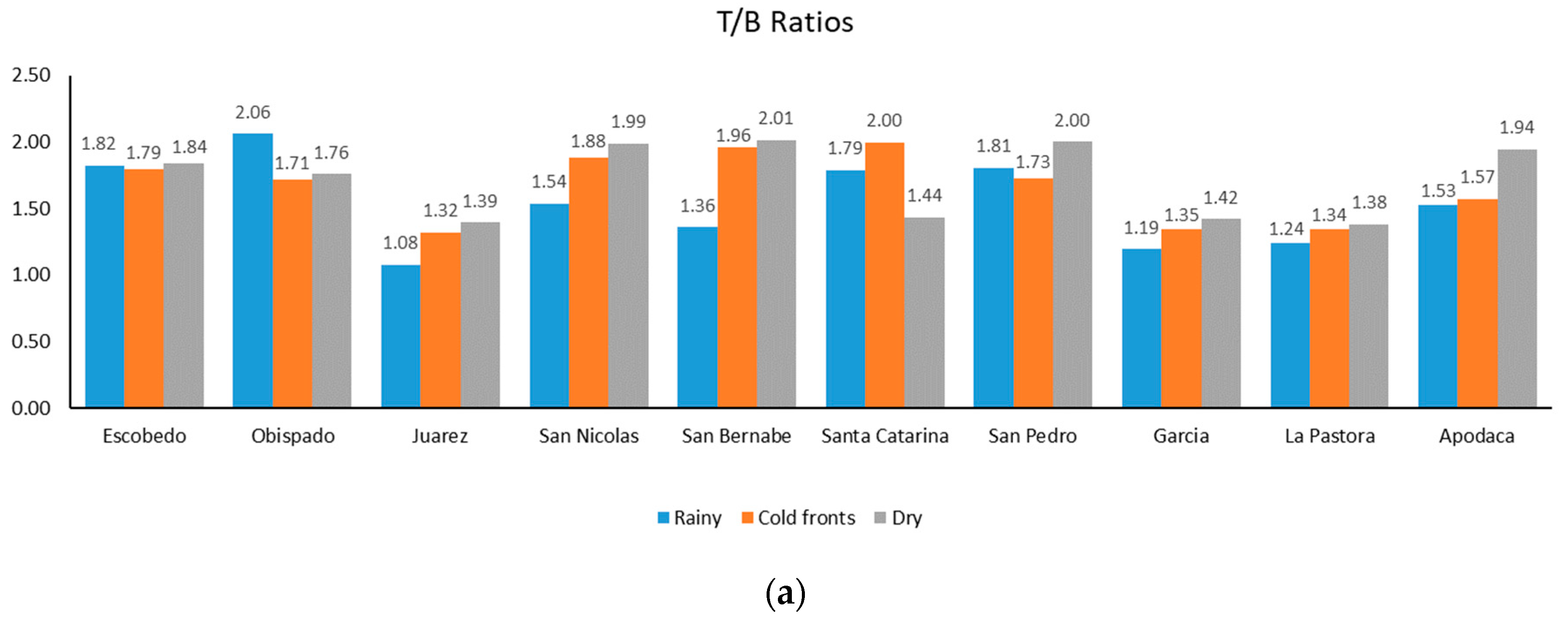
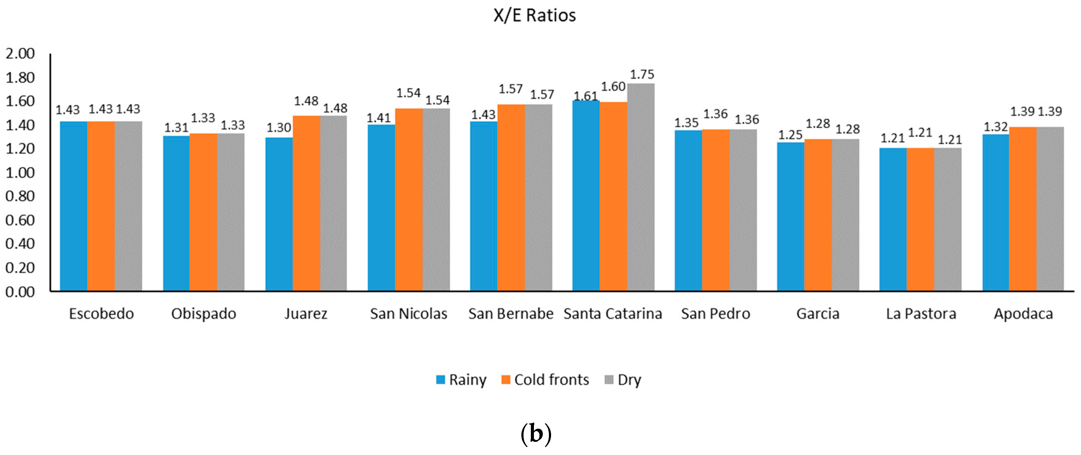
3.5. Aromatic Hydrocarbon Ratios

Aromatic hydrocarbon ratios were computed during the study period to identify the possible sources of the compounds and to gather information about the photochemical processes of air masses.
In a specific site, the toluene/benzene ratio (T/B) is an excellent indicator to determine the relative importance of vehicular emissions as the primary contributors of these compounds. Benzene, toluene, ethylbenzene, and xylene are common air pollutants in urban areas, and a major source of these pollutants is gasoline exhaust. Among these pollutants, both toluene and benzene are the most prevalent components of gasoline. However, toluene can also come from other sources, such as evaporative emissions from coated surfaces, solvent evaporation, service stations, and fuel storage, as well as industrial and area sources [62,63,64]. The T/B ratio is therefore an indicator of the contribution of emissions from vehicular traffic and other sources to the levels of these compounds at the study site.
If the ratio is low, it means that emissions from vehicular traffic are significant, while high values indicate a stronger contribution from sources other than vehicular traffic [65]. In urban environments, a T/B ratio around 1 to 2 is usually associated with fresh vehicular emissions [50].
A T/B ratio greater than 2 indicates that toluene is more abundant than benzene, suggesting the influence of non-traffic-related sources or significant atmospheric transformations. High T/B ratios (greater than 2) are often linked to emissions from industrial activities, solvent use, and painting, rather than direct vehicular exhaust [38]. Toluene is a major component in products such as paints, adhesives, and coatings, as well as in chemical manufacturing, which can lead to elevated emissions in industrial zones. Higher T/B ratios have been observed in areas near industrial facilities or fuel storage locations, where toluene emissions from chemical processes and storage losses dominate over those of benzene [66].
Research indicates that T/B ratios in urban areas with heavy traffic typically range from 1 to 2, as both benzene and toluene are co-emitted from gasoline combustion [67]. In contrast, in industrial zones, T/B ratios often exceed 2, reflecting higher toluene emissions resulting from manufacturing and solvent-related processes [38].
Figure 4a shows that most of the T/B ratios had lower values than 2, except for Obispado during the rainy season, Santa Catarina during the cold fronts season, and San Bernabe and San Pedro during the dry season. The T/B ratios exhibited a range of values from 1.07 to 2.06 for the rainy season, from 1.32 to 1.96 for the cold fronts season, and from 1.38 to 2.01 for the dry season, with mean values of 1.54, 1.66, and 1.72, respectively. The Friedman test was applied, and significant differences were found for these ratios for the three different climatic periods, indicating that this ratio exhibited seasonal behavior. These findings confirm that the aromatic hydrocarbon levels in the MAM are influenced by mixed sources (industrial and vehicular types).
The X/E ratio, first introduced by Nelson and Quigley [68], is widely used to explore aging in air masses. p-xylene and ethylbenzene have atmospheric lifetimes of about 3 h and 8 h, respectively [45]. Due to the faster photochemical disappearance of p-xylene, the X/E ratio decreases with aging. Therefore, higher X/E ratios indicate fresh local emissions, while lower ratios are more commonly associated with photochemical activity and emissions from sources located at a greater distance [64]. Ratios considered “high” are generally reported as approximately 3.0. Previous studies have shown that lower X/E ratios (approximately between 1.0 and 1.5) are typically observed in industrial areas, while higher ratios (approximately between 2.5 and 3.5) are found in traffic areas [37,69].
As can be observed in Figure 4b, the X/E ratio values in this study were lower than 3, ranging from 1.20 to 1.60 for the rainy season, from 1.20 to 1.59 for the cold fronts season, and from 1.20 to 1.74 for the dry season, with mean values of 1.36, 1.41, and 1.44, respectively. After using the Friedman test, it was found that there were no significant differences among the three climatic periods for this ratio. Therefore, it can be concluded that this ratio did not exhibit clear seasonal behavior. The results suggest that the study area was impacted by aged air masses and can be considered typical of industrial areas. Thus, based on this study, it can be inferred that the aromatic hydrocarbon levels in the three climatic seasons could be related not only to industrial and vehicular sources but also to aged emissions.

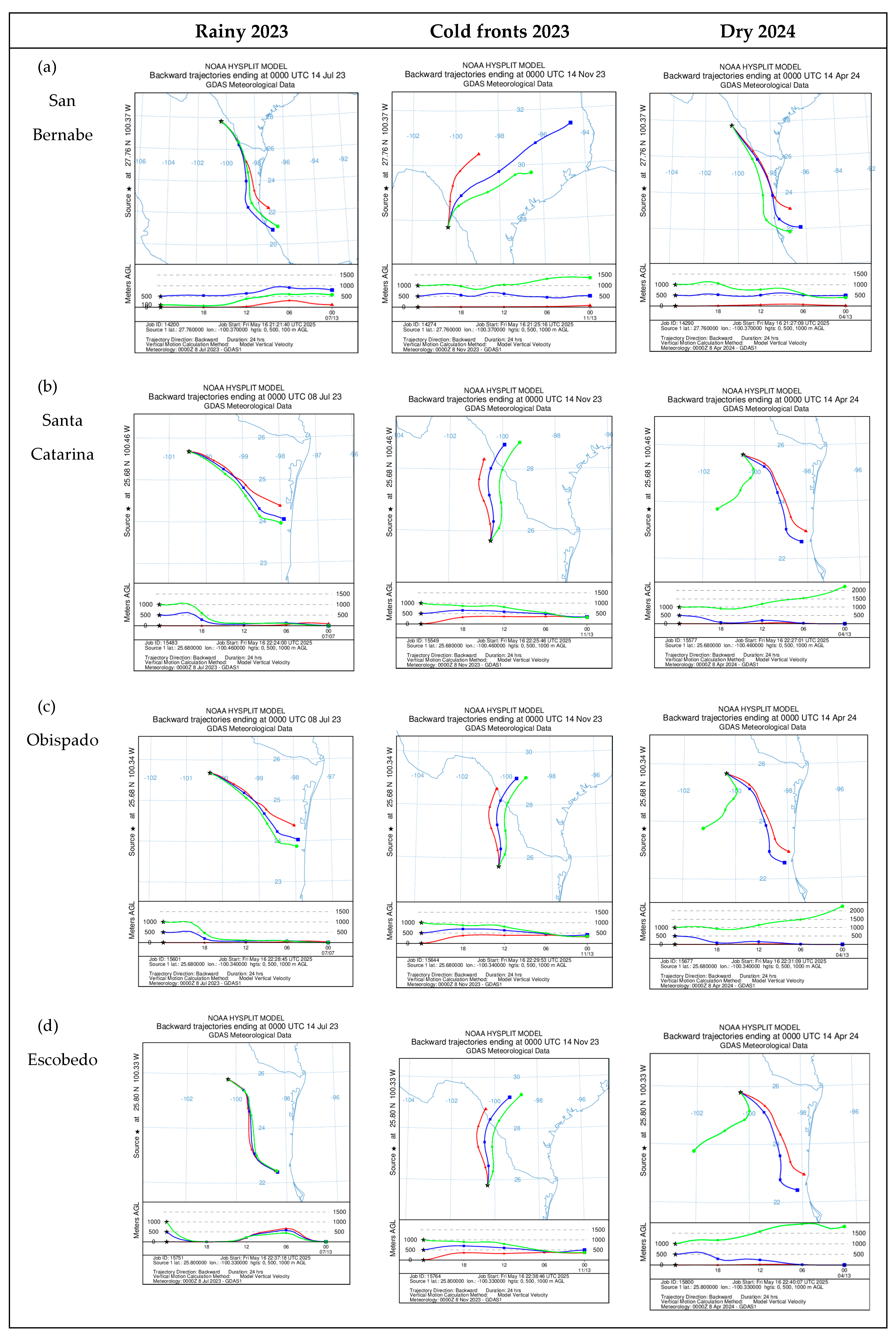
3.6. Backward Air Mass Trajectories

Backward air mass trajectories were calculated for all studied sites during the sampling periods of each climatic season (rainy season of 2023, cold fronts season of 2023, and dry season of 2024) to examine the influence of regional winds on measured air pollutant concentrations. A total of 450 trajectories (10 sites × 15 days × 3 climatic seasons) were computed using HYSPLIT from NOAA. Figure 5 displays representative backward air masses for the sites with the highest concentrations of aromatic hydrocarbons (San Bernabe, Santa Catarina, Obispado, and Escobedo) during the three climatic seasons.
San Bernabe: During the rainy season of 2023, the trajectories show a dominant influence from the southeast, likely associated with maritime air from the Gulf of Mexico. This suggests the presence of more humid air masses with lower pollutant content. In the cold fronts of 2023, transport from the north and northwest reflects the impact of polar air masses, which may reduce local pollutant concentrations due to increased ventilation. In the dry season of 2024, the trajectories indicate a return to a more localized/regional pattern, with recirculation within the valley that could facilitate the accumulation of pollutants.
Santa Catarina: In the rainy season of 2023, air entry is observed from the south and southwest, influenced by the Sierra Madre Oriental. These trajectories may involve cleaner air masses capable of dilution, although interaction with local sources remains possible. During the cold fronts of 2023, trajectories from the north and northeast indicate long-range transport events. In the dry season, recirculated/local trajectories are noted, which increases the potential for pollutant accumulation, particularly under thermal inversion conditions.
Obispado: In the rainy season of 2023, mixed trajectories from both the east and south are observed. Given its central location in the valley, Obispado is influenced by both regional and local factors. During the cold fronts of 2023, air from the northwest and north is noted, with direct trajectories that have a higher potential for transporting pollutants from industrial areas north of the city. In the dry season of 2024, local or stationary trajectories are apparent, reinforcing Obispado’s role as a recipient of aging air masses, which contain a higher proportion of secondary pollutants such as ozone and particles formed by photochemical reactions.
Escobedo: In the rainy season, tracks from the east and northeast are observed, which could bring humid air from the Gulf but might also mix with pollutants transported from industrial or agricultural regions. During the cold fronts in 2023, a dominant northern airflow was recorded, potentially leading to atmospheric clearing depending on wind speed. In the dry season, closed/local tracks are observed, favoring the accumulation of pollutants emitted by local sources (such as industry and traffic) and chemical transformation processes.
During the rainy season, concentrations of aromatic hydrocarbons were lower due to the influx of more humid air masses with reduced pollutant content, resulting from a washout effect. During the cold fronts of 2023, long-range transported air may have influenced the levels of toluene, benzene, and ethylbenzene, leading to higher concentrations of these pollutants since their atmospheric half-lives (at ~1.5 × 10⁶ molecules/cm3) are approximately 1.9–2.3 days for toluene, 9–12 days for benzene, and 1.4–1.6 days for ethylbenzene. High levels of p-xylene (atmospheric half-life 6–8 h), combined with local winds during the dry season of 2024, indicate that recent local sources played a significant role during this sampling period.

3.7. Health Risk Assessment Results

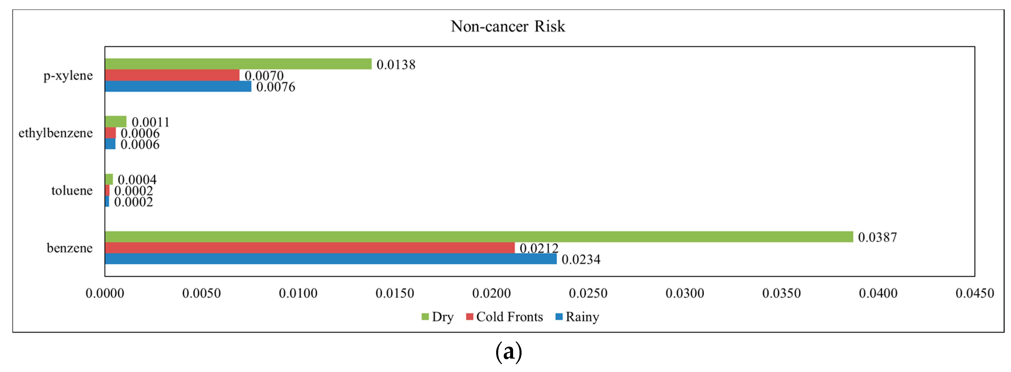
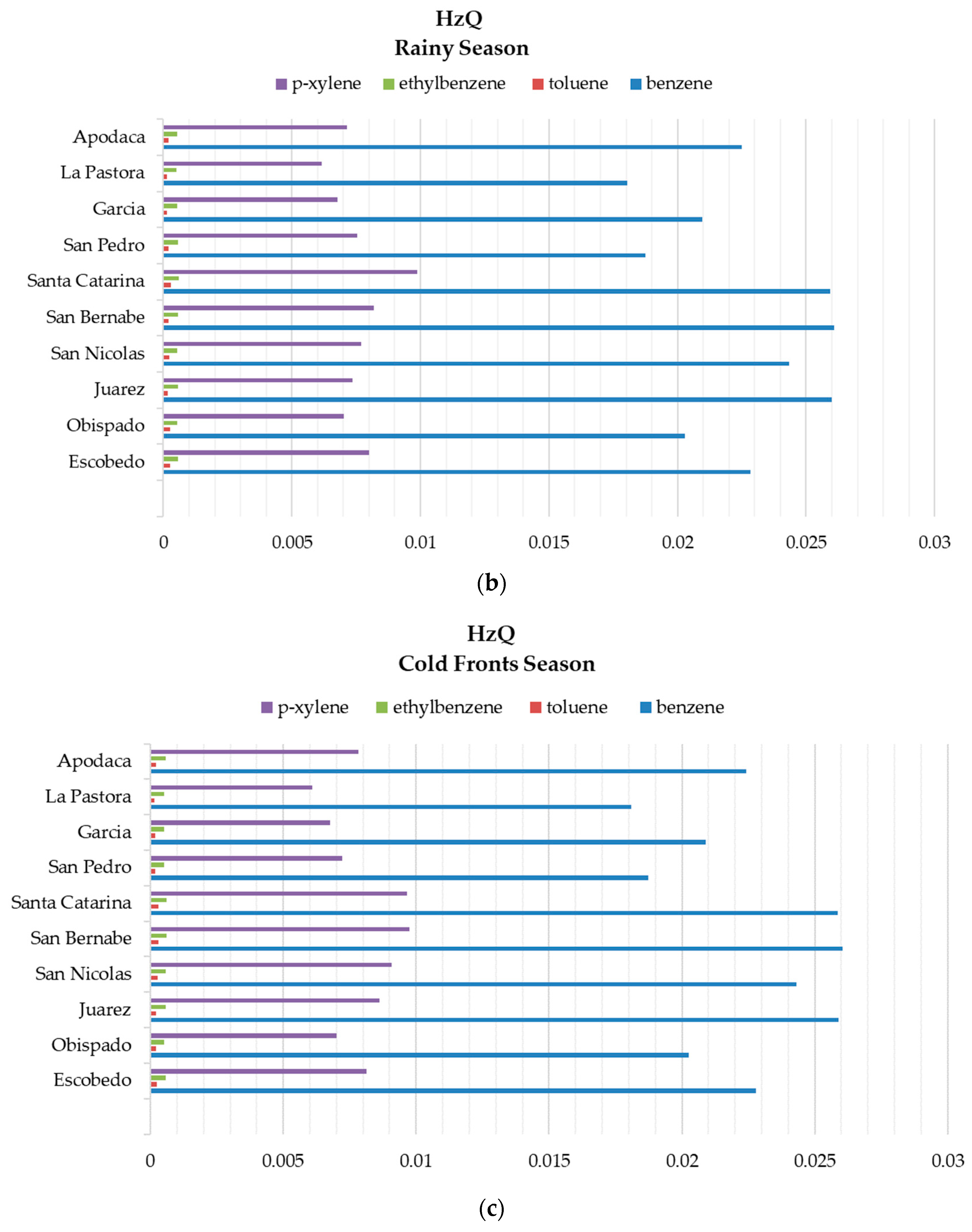
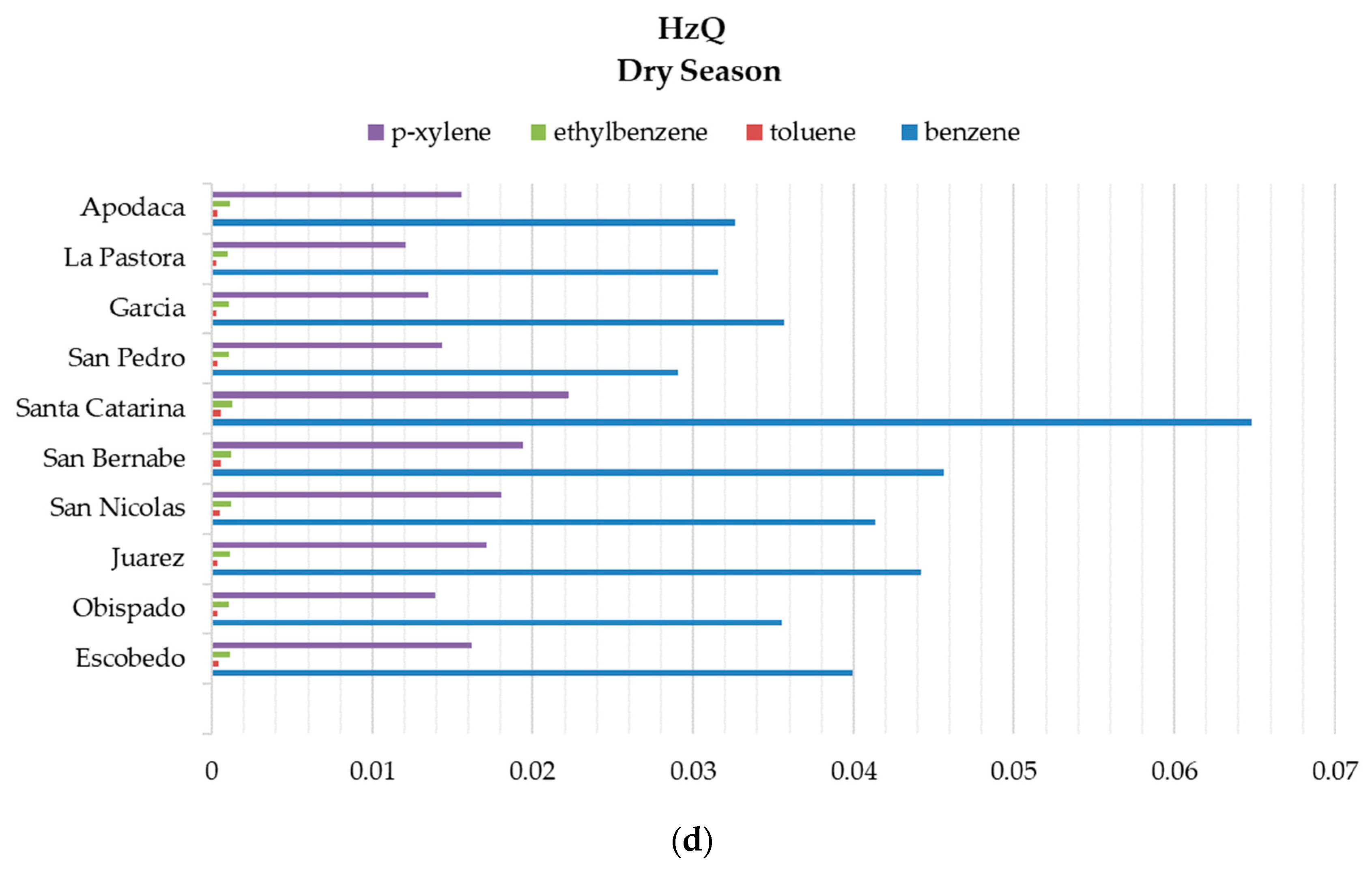
3.7.1. Non-Cancer Risk

The HzQ quotient is a tool used to estimate whether a population is exposed to a daily dose of pollutants exceeding the maximum safe levels set to protect their health. A HzQ value greater than 1 indicates that the population may suffer from chronic diseases, such as respiratory and circulatory diseases, due to long-term exposure to these pollutant levels [70]. In the case of the MAM, the values for each climatic season are shown in Figure 6, with all of them lower than 1, which means that the population in the MAM is not at risk of suffering from chronic diseases. It should be noted that benzene had the highest HzQ values during the three climatic seasons. In this study, the integrated non-cancer risk index (HzQ) values (sum of the individual HzQ values for each compound) were 0.031 (rainy season), 0.029 (cold fronts season), and 0.054 (dry season), with the highest values observed during the dry season. The results indicate that the non-carcinogenic health risk presents a seasonal variation, with the highest risk observed during the dry season (HzQ = 0.054). In this season, high-pressure systems reduce atmospheric dispersion, causing air pollutants to accumulate [71]. Additionally, the lack of rainfall limits the removal of airborne pollutants, which increases exposure risks [72]. Higher temperatures can enhance the evaporation of volatile organic compounds (VOCs), contributing to respiratory and neurological effects [73].
During the rainy season, an integrated HzQ value of 0.031 was recorded, indicating a moderate risk. Lower temperatures and frequent rainfalls facilitate the better dispersion of pollutants, thereby reducing their accumulation in the air [35]. However, thermal inversions can trap pollutants near the ground, potentially leading to localized increases in HzQ values [33].
The lowest integrated HzQ value was found during the cold front season, with a value of 0.029, indicating the lowest risk. Stronger winds occurring in this season remove pollutants from the atmosphere. Higher humidity levels and greater atmospheric mixing promote dilution, which further lowers exposure risks [34].
It can be inferred that vulnerable populations—such as children, the elderly, and individuals with respiratory diseases—are at greater risk of adverse effects during the dry season [35].
The integrated values for HzQ were higher than those reported in Iran (0.0186) [74] and in Delhi, India (0.02576) [75] but lower than those reported for Kuala Lumpur, Malaysia (0.6221) [76]. HzQ values showed the following ranges: from 0.01805 to 0.0648 for benzene; from 0.00013 to 0.00055 for toluene; from 0.00050 to 0.00127 for ethylbenzene; and from 0.0060 to 0.02223 for p-xylene.
As mentioned above, HzQ did not exceed the value of 1.0; however, it is important to assess the variability found in sampling sites, climatic seasons, and each compound. HzQ values were lower during the rainy season (Figure 6a), which agrees with the exposure doses found, considering that during the rainy season, the dilution effect decreases the concentrations in ambient air and therefore decreases the associated risk. In Figure 6b, HzQ values for each sampling site are shown for the rainy season. It can be observed that risk values for benzene were higher in Juarez, San Bernabe, and Santa Catarina; this agrees with the exposure doses observed since the highest benzene concentrations were found in these sites. For toluene, the highest values for HzQ were observed in Obispado, Santa Catarina, and Escobedo. HzQ values during the rainy season were higher for ethylbenzene in Santa Catarina, Juarez, and Escobedo. p-xylene showed the highest values for HzQ during the rainy season for Santa Catarina, San Bernabe, and Escobedo. Figure 6c shows the HzQ values for each sampling site during the cold fronts season. Benzene showed the highest HzQ values in Santa Catarina, San Bernabe, and Juarez. Toluene, ethylbenzene, and xylene showed the same behavior, presenting the highest values for HzQ in Santa Catarina, San Bernabe, and San Nicolas. Figure 6d shows the HzQ values for each sampling site during the dry season. Santa Catarina and San Bernabe showed the highest HzQ values for benzene and toluene. In the case of ethylbenzene, Santa Catarina, San Bernabe, Apodaca, Juarez, and Escobedo registered the highest HzQ values. Finally, Santa Catarina and San Nicolas registered the highest non-cancer risk coefficients for p-xylene.

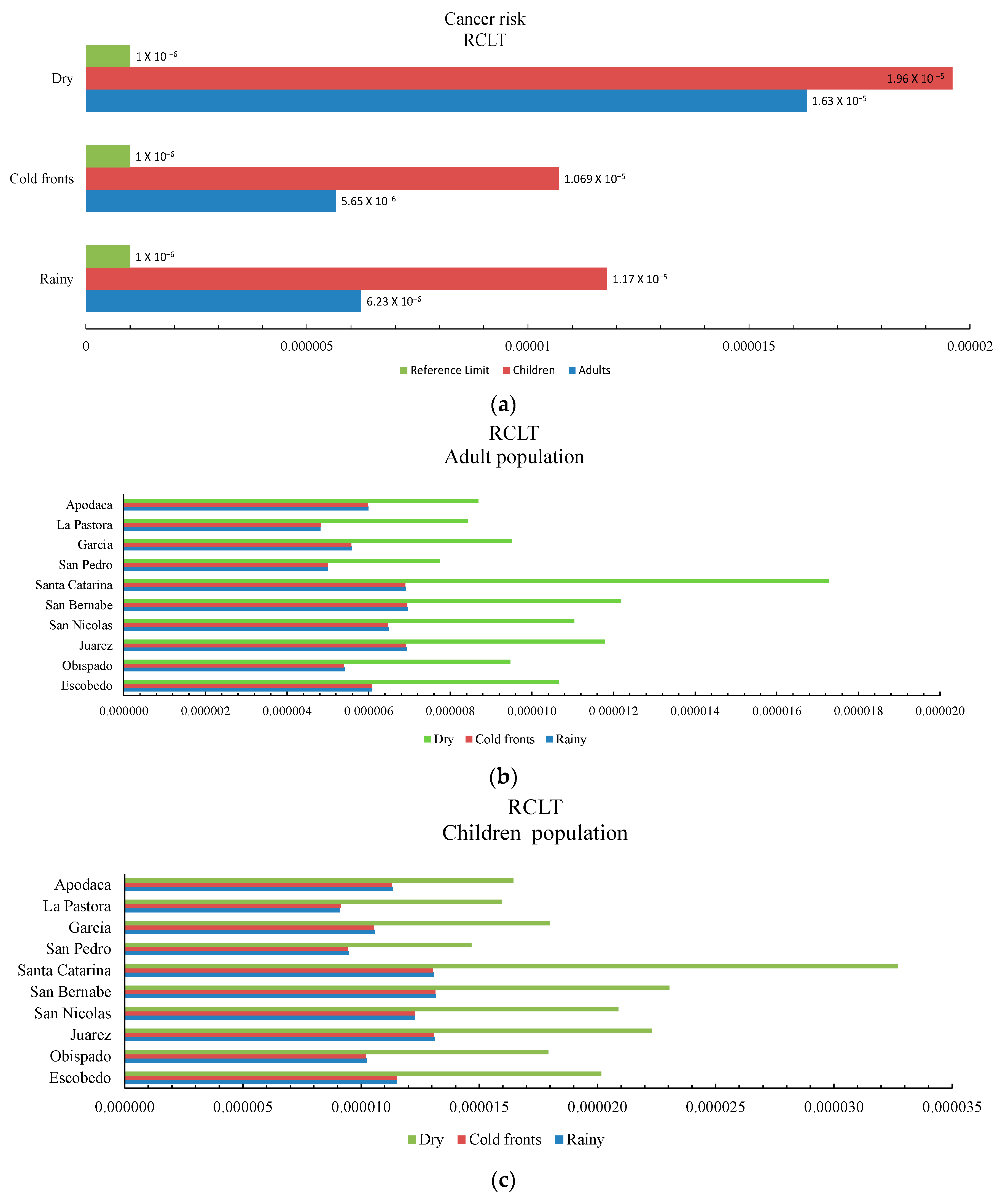
3.7.2. Carcinogenic Risk

In Figure 7a, the values obtained for cancer risk (RCLT) from benzene are shown by sampling season. As can be observed, in all climatic seasons and in both population groups, benzene levels exceeded the reference limit established by the EPA [28] for cancer risk (1 × 10⁻⁶). RCLT values ranged from 9.11 × 10⁻⁶ to 1.32 × 10⁻⁵, from 9.13 × 10⁻⁶ to 1.31 × 10⁻⁵, and from 1.47 × 10⁻⁵ to 3.27 × 10⁻⁵ for the rainy, the cold fronts, and the dry seasons, respectively, for the child population. Whereas for the adult population, RCLT values ranged from 4.81 × 10⁻⁶ to 6.96 × 10⁻⁶, from 4.82 × 10⁻⁶ to 6.94 × 10⁻⁶, and from 7.75 × 10⁻⁶ to 1.73 × 10⁻⁵ for the rainy, the cold fronts, and the dry seasons, respectively. Applying the Friedman test, we found significant differences between the rainy and the cold fronts seasons compared to the dry season in RCLT values for both children and adults. The mean values estimated in this study for RCLT were 7.56 × 10⁻⁶ and 1.43 × 10⁻⁵, for the adult and child populations, respectively. These values are higher than those reported in Tehran, Iran (3.97 × 10⁻⁷) [74], Düzce, Turkey (9 × 10⁻⁶ for a rural area) [77], and Aliaga, Turkey (12.9 × 10⁻⁶) [77], and lower than those found in Delhi, India (6.1 × 10⁻⁵) [75], Düzce, Turkey (2 × 10⁻⁵ for an industrial area) [77], and Tehran, Iran (2 × 10⁻⁵) [78].
As can be observed from Figure 7b, the cancer risk for adults exceeded the reference limit established by the US EPA [26] in all municipalities, being higher in San Nicolas, San Bernabe, Juarez, and Santa Catarina, whereas the risk was lower in rural sites like La Pastora. In Figure 7c, it can be observed that cancer risk values for the child population had a seasonal behavior, showing higher values of RCLT in the dry season. The highest values of the cancer risk coefficient were found in Juarez, San Nicolas, San Bernabe, and Santa Catarina, which agrees with industrial activities and vehicular traffic prevailing in these municipalities. It can be observed that, in all sampling sites and climatic seasons, the cancer risk values were significantly higher for the child population, in particular, in Juarez, San Nicolas, San Bernabe, and Santa Catarina. This is an important finding from the point of view of public health.

4. Conclusions

This study examined the spatiotemporal distribution of aromatic hydrocarbons (benzene, toluene, ethylbenzene, and p-xylene) across ten locations in the Metropolitan Area of Monterrey (MAM), Mexico. Passive sampling techniques were employed during three distinct climatic seasons: the rainy season of 2023, the cold front season of 2023, and the dry season of 2024. The relative abundance of the measured compounds in the MAM for the three climatic seasons (the rainy, the cold fronts, and the dry seasons) was toluene > p-xylene > benzene > ethylbenzene.
The results indicated that the aromatic hydrocarbon concentrations were highest during the dry season. This increase is likely due to lower wind speeds, atmospheric stagnation, higher emissions, and reduced wet deposition. In contrast, the rainy season exhibited the lowest levels of these compounds in the atmosphere. This suggests that the heavy rains during the rainy season played a significant role in diluting air pollutant concentrations. Wet seasons (both rainy and cold fronts) typically involve heavy rainfall and drizzle. These conditions contribute to the dilution and reduction in the aromatic hydrocarbon levels at ground level. Moreover, unstable atmospheric conditions during these periods promote mixing and aid in the dispersion of pollutants in the atmosphere. Consequently, we can conclude that the seasonal and spatial variability in aromatic hydrocarbon concentrations can be attributed to the following factors: the dilution effect during the rainy season, increased atmospheric stability during the dry season, industrial and vehicular emissions, and the presence of aged air masses.
Benzene and its alkyl derivatives (toluene, ethylbenzene, and p-xylene) were found to be higher in areas with high industrial and commercial activity, where heavy vehicular traffic is common. Santa Catarina and San Bernabe consistently exhibited the highest levels of these compounds, indicating significant impacts from industrial activities, heavy vehicular traffic, and urban emissions.
This study indicates that there were correlations between the aromatic hydrocarbons, suggesting that their sources were likely common during the study period. The aromatic hydrocarbon ratios identified in this research suggest that the measured compounds were linked to a mix of sources, including both industrial and vehicular emissions. The ratios fell within the typical range associated with vehicular emissions in urban areas; however, some sampling sites revealed influences from sources beyond just vehicular traffic. Specifically, these influences were noted at Obispado during the rainy season, Santa Catarina during cold fronts, and San Pedro and San Bernabe during the dry season. On the other hand, the values found for the X/E ratio indicate that the measured pollutants were associated with aged air masses and industrial emissions. It is important to note that the study area is a complex area in which different types of emission sources co-exist.
There was a marked spatial variability in the concentration of aromatic hydrocarbons, except for benzene, which was found to be very uniform in all municipalities of the MAM. This variability indicates that the industrial activities and vehicular traffic associated with each municipality played a significant role in this behavior. An analysis of the toluene/benzene (T/B) ratio indicated mixed pollution sources, with certain locations showing values greater than 2. This suggests contributions from industrial and solvent-related sources, in addition to vehicular emissions.
According to the health risk assessment, the residents in the vicinity of the MAM were not exposed to any significant health risks, other than cancer, during the sampling period. However, benzene was found to be the most hazardous compound, with the highest HzQ values, especially in areas like Juarez, San Bernabe, and Santa Catarina. It was found that the cancer risk values (RCLT) in both children and adults due to long-term exposure to benzene during all seasons surpassed the limit set by the EPA for cancer risk (1 × 10⁻⁶). These values were significantly higher in areas with high industrial and vehicular traffic, such as San Nicolas, San Bernabe, Juarez, and Santa Catarina. It is worth noting that cancer risk values were much higher in children as compared to adults, indicating that children are at a higher risk of developing cancer due to atmospheric pollution, particularly due to benzene exposure in the MAM. This study highlights the necessity for the continuous monitoring of the levels of these air pollutants, as current air quality monitoring networks in the MAM do not measure these pollutants, leading to an underestimation of their impact on health and the environment. The high concentrations of aromatic hydrocarbons in industrial and high-traffic areas underline the pressing need for regulatory measures, emission control strategies, and enhanced monitoring networks.

Author Contributions

Conceptualization, J.G.C.B. and R.M.C.B.; data curation, C.M.R. and A.A.E.G.; formal analysis, C.A.A.U. and M.d.l.L.E.F.; investigation, R.M.C.B.; methodology, C.A.A.U. and M.P.U.C.; project administration, J.G.C.B. and R.M.C.B.; resources, J.G.C.B.; software, C.A.A.U., C.M.R. and A.A.E.G.; supervision, S.E.C.L. and M.d.l.L.E.F.; validation, C.M.R. and S.E.C.L.; visualization, A.A.E.G.; writing—original draft, J.G.C.B., R.M.C.B. and E.R.L.; writing—review and editing, J.G.C.B. and R.M.C.B. All authors have read and agreed to the published version of the manuscript.

Funding

This research received no external funding.

Institutional Review Board Statement

Not applicable.

Informed Consent Statement

Not applicable.

Data Availability Statement

The datasets generated for the current study are not publicly available but are available from the corresponding author on reasonable request.

Acknowledgments

The authors thank the Atmospheric Monitoring System of Monterrey (SIMA) for its logistical and technical support.

Conflicts of Interest

The authors declare no conflicts of interest.

References

  1. Alford, K.L.; Kumar, N. Pulmonary Health Effects of Indoor Volatile Organic Compounds-A Meta-Analysis. Int. J. Environ. Res. Public Health 2021, 18, 1578. [Google Scholar] [CrossRef] [PubMed] [PubMed Central]
  2. Hawari, N.S.L.L.; Latif, M.T.; Hamid, H.H.; Leng, T.H.; Othman, M.; Mohtar, A.A.A.; Azhar, A.; Dominick, D. The concentration of BTEX in selected urban areas of Malaysia during the COVID-19 pandemic lockdown. Urban Clim. 2022, 45, 101238. [Google Scholar] [CrossRef] [PubMed]
  3. Atkinson, R. Gas-phase tropospheric chemistry of organic compounds: A review. Atmos. Environ. 2007, 41, 200–240. [Google Scholar] [CrossRef]
  4. US EPA, Environmental Protection Agency. Technical Overview of Volatile Organic Compounds (VOCs). 2022. Available online: https://www.epa.gov/indoor-air-quality-iaq/technical-overview-volatile-organic-compounds (accessed on 30 October 2024).
  5. IARC, International Agency for Research on Cancer. Benzene–IARC Monographs on the Evaluation of Carcinogenic Risks to Humans; World Health Organization: Geneva, Switzerland, 2018; Volume 120, Available online: https://publications.iarc.fr/Book-And-Report-Series/Iarc-Monographs-On-The-Identification-Of-Carcinogenic-Hazards-To-Humans/Benzene-2018 (accessed on 30 November 2024).
  6. Civan, M.Y.; Elbir, T.; Seyfioglu, R.; Kuntasal, O.O.; Bayram, A.; Dogan, G.; Yurdakul, S.; Andic, O.; Muezzinoglu, A.; Sofuoglu, S.C.; et al. Spatial and temporal variations in atmospheric VOCs, NO2, SO2, and O3 concentrations at a heavily industrialized region in Western Turkey, and assessment of the carcinogenic risk levels of benzene. Atmos. Environ. 2015, 103, 102–113. [Google Scholar] [CrossRef]
  7. INECC, Instituto Nacional de Ecología y Cambio Climático; National Institute of Ecology and Climatic Change. Informe Nacional de Calidad del Aire 2018; Coordinación General de Contaminación y Salud Ambiental, Dirección de Investigación de Calidad del Aire y Contaminantes: Ciudad de México, México, 2019; Available online: http://140.84.163.2:8080/xmlui/handle/publicaciones/346 (accessed on 25 November 2024).
  8. INEGI, Instituto Nacional de Estadística, Geografía e Informática; National Institute of Statistics, Geography and Informatics. Registered Motor Vehicles in Circulation (VMRC). Estado de Nuevo León. 2025. Available online: https://en.www.inegi.org.mx/programas/vehiculosmotor/ (accessed on 29 November 2024).
  9. Cocheo, V.; Boaretto, C.; Sacco, P. High uptake rate radial diffusive sampler suitable for both solvent and thermal desorption. Am. Ind. Hyg. Assoc. J. 1996, 57, 897–909. [Google Scholar] [CrossRef]
  10. Healy, R.M.; Bennett, J.; Wang, J.M.; Karellas, N.S.; Wong, C.; Todd, A.; Sofowote, U.; Su, Y.; Di Federico, L.; Munoz, A.; et al. Evaluation of a passive sampling method for long-term continuous monitoring of volatile organic compounds in urban environments. Environ. Sci. Technol. 2018, 52, 10580–10589. [Google Scholar] [CrossRef]
  11. Sekar, A.; Varghese, G.K.; Varma, M.R. Analysis of benzene air quality standards, monitoring methods and concentrations in indoor and outdoor environment. Heliyon 2019, 5, e02918. [Google Scholar] [CrossRef]
  12. Chaiklieng, S.; Suggaravetsiri, P.; Kaminski, N.; Autrup, H. Exposure to benzene and toluene of gasoline station workers in Khon Kaen, Thailand and adverse effects. Hum. Ecol. Risk Assess. Int. J. 2021, 27, 1823–1837. [Google Scholar] [CrossRef]
  13. Cruz, L.P.; Alves, L.P.; Santos, A.V.; Esteves, M.B.; Gomes, I.V.; Nunes, L.S. Assessment of BTEX concentrations in air ambient of gas stations using passive sampling and the health risks for workers. J. Environ. Prot. 2017, 8, 12–21. [Google Scholar] [CrossRef]
  14. CONAPO, Consejo Nacional de Población. National Council of Population. Delimitación de Zonas Metropolitanas de México 2015, México. 2015. Available online: https://www.gob.mx/cms/uploads/attachment/file/305634/Delimitacion_Zonas_Metropolitanas_2015.pdf (accessed on 25 November 2024).
  15. Safronievska, I.; Petrska, J.; Bogdanov, J.; Stefova, M. Assay of volatile organic compounds in urban air using passive sampling and gas chromatography coupled to mass spectrometry. Maced. J. Ecol. Environ. 2022, 24, 103–113. [Google Scholar] [CrossRef]
  16. Huang, C.; Tang, L.; Dai, X.; Xiao, H. Evaluation and application of a passive air sampler for atmospheric volatile organic compounds. Aerosol Air Qual. Res. 2018, 18, 3047–3055. [Google Scholar] [CrossRef]
  17. INSHT, Instituto Nacional de Seguridad e Higiene en el Trabajo; National Institute of Safety and Hygiene. Determinación de Hidrocarburos Aromáticos (Benceno, Tolueno, Etilbenceno, p-Xileno, 1,2,4-Trimetilbenceno) en Aire-Método de Adsorción en Carbón Activo/Cromatografía de Gases; MTA/MA-030/A92; Ministerio del Trabajo y Asuntos Sociales de España: Madrid, Spain, 1992. [Google Scholar]
  18. EN 14662-5:2005; Ambient Air Quality. Standard Method for Measurement Of Benzene Concentrations. Diffusive Sampling Followed By Solvent Desorption And Gas Chromatography. British Standard: London, UK, 2010.
  19. Fondelli, M.C.; Bavazzano, P.; Grechi, D.; Gorini, G.; Miligi, L.; Marchese, G.; Cenni, I.; Scala, D.; Chellini, E.; Constantini, A.S. Benzene exposure in a sample of population residing in a district of Florence, Italy. Sci. Total Environ. 2008, 392, 41–49. [Google Scholar] [CrossRef] [PubMed]
  20. Cerón, J.G.; Cerón, R.M.; Martínez, S.; Kahl, J.; Guarnaccia, C.; Lara, R.C.; Rangel, M.; Ramírez, E.; Espinosa, M.L.; Uc, M.P.; et al. Health risk assessment of the levels of BTEX in ambient air of one urban site located in Leon, Guanajuato, Mexico during two climatic seasons. Atmosphere 2020, 11, 165. [Google Scholar] [CrossRef]
  21. Pekey, B.; Yılmaz, H. The use of passive sampling to monitor spatial trends of volatile organic compounds (VOCs) at an industrial city of Turkey. Microchem. J. 2011, 97, 213–219. [Google Scholar] [CrossRef]
  22. Keymeulen, R. Benzene, toluene, ethyl benzene and xylenes in ambient air and Pinus sylvestris L. needles: A comparative study between Belgium, Hungary, and Latvia. Atmos. Environ. 2001, 35, 6327–6335. [Google Scholar] [CrossRef]
  23. Li, Y.; Yan, Y.; Hu, D.; Li, Z.; Hao, A.; Li, R.; Peng, L. Source apportionment of atmospheric volatile aromatic compounds (BTEX) by stable carbon isotope analysis: A case study during heating period in Taiyuan, northern China. Atmos. Environ. 2020, 225, 117369. [Google Scholar] [CrossRef]
  24. WRPLOT View, v.8.0.2, Lakes Environmental Software; Lakes Environmental Inc.: Waterloo, ON, Canada, 2018.
  25. U.S. NOAA, HYSPLIT Model. Hybrid Single-Particle Lagrangian Integrated Trajectory Model. 2021. Available online: https://www.arl.noaa.gov/hysplit (accessed on 20 November 2024).
  26. Shaw, R.G.; Mitchell-Olds, T. ANOVA for unbalanced data: An overview. Ecology 1993, 74, 1638–1645. [Google Scholar] [CrossRef]
  27. Helsel, D.R.; Hirsch, R.M. Statistical Methods in Water Resources. U.S. Geological Survey Techniques of Water-Resources Investigations; U.S. Geological Survey: Reston, VA, USA, 2002. [Google Scholar]
  28. Hair, J.F.; Anderson, R.E.; Tatham, R.L.; Black, W.C. Multivariate Data Analysis, 5th ed.; Prentice Hall: Upper Saddle River, NJ, USA, 1998. [Google Scholar]
  29. US EPA, Environmental Protection Agency. Integrated Risk Information System (IRIS). Toxicological Review of Benzene (Non-Cancer Effects) (EPA/635/R-02/001F). 2014. Available online: https://iris.epa.gov/static/pdfs/0276tr.pdf (accessed on 25 November 2024).
  30. Zhang, Z.; Wang, X.; Zhang, Y.; Lu, S.; Huang, Z.; Huang, X.; Wang, Y. Ambient air benzene at background sites in China’s most developed coastal regions: Exposure levels, source implications and health risks. Sci. Total Environ. 2015, 511, 792–800. [Google Scholar] [CrossRef]
  31. US EPA, Environmental Protection Agency. Compendium Method TO-14A. Determination of Volatile Organic Compounds (VOCs) in Ambient Air Using Specially Prepared Canisters with Subsequent Analysis by Gas Chromatography. 1999. Available online: https://www.epa.gov/sites/default/files/2019-11/documents/to-14ar.pdf (accessed on 25 November 2024).
  32. US EPA, Environmental Protection Agency. Passive Samplers for Investigations of Air Quality: Method Description, Implementation, and Comparison to Alternative Sampling Methods. 1999. Available online: https://nepis.epa.gov/Adobe/PDF/P100MK4Z.pdf (accessed on 25 November 2024).
  33. Nejad, M.T.; Ghalehteimouri, K.J.; Talkhabi, H.; Dolatshahi, Z. The relationship between atmospheric temperature inversion and urban air pollution characteristics: A case study of Tehran, Iran. Discov. Environ. 2023, 1, 1–17. [Google Scholar] [CrossRef]
  34. Elminir, H.K. Dependence of urban air pollutants on meteorology. Sci. Total Environ. 2005, 350, 225–237. [Google Scholar] [CrossRef]
  35. Yang, J.; Shi, B.; Shi, Y.; Marvin, S.; Zheng, Y.; Xia, G. Air pollution dispersal in high density urban areas: Research on the triadic relation of wind, air pollution, and urban form. Sustain. Cities Soc. 2020, 54, 101941. [Google Scholar] [CrossRef]
  36. INEGI, Instituto Nacional de Estadística, Geografía e Informática. National Institute of Statistics, Geography and Informatics. Cuéntame INEGI, Información por Entidad. Estado de Nuevo León. 2020. Available online: http://cuentame.inegi.org.mx/monografias/informacion/nl/default.aspx?tema=me&e=19 (accessed on 10 December 2024).
  37. Monod, A.; Sive, B.C.; Avino, P.; Chen, T.; Blake, D.R.; Rowland, F.S. Monoaromatic compounds in ambient air of various cities: A focus on correlations between the xylenes and ethylbenzene. Atmos. Environ. 2001, 35, 135–149. [Google Scholar] [CrossRef]
  38. Wang, H.; Qiao, Y.; Chen, C.; Lu, J.; Dai, H.; Qiao, L.; Lou, S.; Huang, C.; Li, L.; Jing, S.; et al. Source profiles and chemical reactivity of volatile organic compounds from solvent use in Shanghai, China. Aerosol Air Qual. Res. 2014, 14, 301–310. [Google Scholar] [CrossRef]
  39. INECC, Instituto Nacional de Ecología y Cambio Climático. National Institute of Ecology and Climate Change. Emissions inventory of Monterrey Metropolitan Area. 2019. Available online: http://aire.nl.gob.mx/docs/reportes/PIGECA_2023_2033.pdf (accessed on 15 November 2024).
  40. Galindo, J.; Climent, H.; de la Morena, J.; González-Domínguez, D.; Guilain, S.; Besançon, T. Assessment of air-management strategies to improve the transient performance of a gasoline engine under high EGR conditions during load-decrease operation. Int. J. Engine Res. 2023, 24, 506–520. [Google Scholar] [CrossRef]
  41. INECC, Instituto Nacional de Ecología y Cambio Climático. National Institute of Ecology and Climatic Change. Evaluación de Compuestos Orgánicos Volátiles en el Área Metropolitana de Monterrey. 2015. Available online: https://www.gob.mx/cms/uploads/attachment/file/370440/8._Informe_Final_de_COVs_Monterrey.pdf (accessed on 16 November 2022).
  42. Hamid, H.H.A.; Latif, M.T.; Nadzir, M.S.M.; Uning, R.; Khan, F.; Kannan, N. Ambient BTEX levels over urban, suburban, and rural areas in Malaysia. Air Qual. Atmos. Health 2019, 12, 341–351. [Google Scholar] [CrossRef]
  43. Hatakeyama, S.; Kobayashi, H.; Akimoto, H. Gas-phase oxidation of sulfur dioxide in the ozone-olefin reactions. J. Phys. Chem. 1984, 88, 4736–4739. [Google Scholar] [CrossRef]
  44. Liu, T.; Chan, A.W.H.; Abbatt, J.P.D. Multiphase Oxidation of Sulfur Dioxide in Aerosol Particles: Implications for Sulfate Formation in Polluted Environments. Environ. Sci. Technol. 2021, 55, 4227–4242. [Google Scholar] [CrossRef]
  45. Atkinson, R. Atmospheric chemistry of VOCs and NOx. Atmos. Environ. 2000, 34, 2063–2101. [Google Scholar] [CrossRef]
  46. Słomińska, M.; Konieczka, P.; Namieśnik, J. The Fate of BTEX Compounds in Ambient Air. Crit. Rev. Environ. Sci. Technol. 2014, 44, 455–472. [Google Scholar] [CrossRef]
  47. Jia, M.; Zhao, T.; Cheng, X.; Gong, S.; Zhang, X.; Tang, L.; Liu, D.; Wu, X.; Wang, L.; Chen, Y. Inverse relations of PM2.5 and O3 in air compound pollution between cold and hot seasons over an urban area of East China. Atmosphere 2017, 8, 59. [Google Scholar] [CrossRef]
  48. Ballard, L.P.; Matus, L.K. A Study of Correlations of Ozone and Sulfur Dioxide; Report EPA-R3-72-013; Research Triangle Institute: Research Triangle Park, NC, USA, 1972. [Google Scholar]
  49. Wilson, W.E.; Levy, A.; Wimmer, D.B. A study of sulfur dioxide in photochemical smog II. Effect of sulfur dioxide on oxidant formation in photochemical smog. J. Air Pollut. Control Ass. 1972, 22, 27–32. [Google Scholar] [CrossRef] [PubMed]
  50. Khoder, M.I. Ambient levels of volatile organic compounds in the atmosphere of Greater Cairo. Atmos. Environ. 2007, 41, 554–566. [Google Scholar] [CrossRef]
  51. Liu, A.; Hong, N.; Zhu, P.; Guan, Y. Understanding benzene series (BTEX) pollutant load characteristics in the urban environment. Sci. Total Environ. 2018, 619, 938–945. [Google Scholar] [CrossRef]
  52. Yu, B.; Yuan, Z.; Yu, Z.; Xue, F. BTEX in the environment: An update on sources, fate, distribution, pretreatment, analysis, and removal techniques. Chem. Eng. J. 2022, 435, 134825. [Google Scholar] [CrossRef]
  53. Liu, C.; Xin, Y.; Zhang, C.; Liu, J.; Liu, P.; He, X.; Mu, Y. Ambient volatile organic compounds in urban and industrial regions in Beijing: Characteristics, source apportionment, secondary transformation and health risk assessment. Sci. Total Environ. 2023, 855, 158873. [Google Scholar] [CrossRef]
  54. Li, G.; Deng, S.; Li, J.; Gao, J.; Lu, Z.; Yi, X.; Liu, J. Levels, ozone and secondary organic aerosol formation potentials of BTEX and their health risks during autumn and winter in the Guanzhong Plain, China. Air Qual. Atmos. Health 2022, 15, 1941–1952. [Google Scholar] [CrossRef]
  55. Kerminen, V.-M.; Pirjola, L.; Boy, M.; Eskola, A.; Teinilä, K.; Laakso, L.; Asmi, A.; Hienola, J.; Lauri, A.; Vainio, V.; et al. Interaction between SO2 and submicron atmospheric particles. Atmos. Res. 2000, 54, 41–57. [Google Scholar] [CrossRef]
  56. Yudison, A.; Driejona, D. Determination of BTEX concentration using passive samplers in a heavy traffic area of Jakarta, Indonesia. Int. J. Geomate 2020, 19, 180–187. [Google Scholar] [CrossRef]
  57. Kheirbek, I.; Johnson, S.; Ross, Z.; Pezeshki, G.; Ho, K.; Eisl, H.; Matte, T. Spatial variability in levels of benzene, formaldehyde, and total benzene, toluene, ethylbenzene and xylenes in New York City: A land-use regression study. Environ. Health 2012, 11, 51. [Google Scholar] [CrossRef]
  58. Moolla, R.; Johnson, R.S. Spatial distribution of ambient BTEX concentrations at an International Airport in South Africa. Int. J. Environ. Ecol. Eng. 2019, 13, 43–50. [Google Scholar]
  59. Son, B.; Breysse, P.; Yong, W. Volatile organic compounds concentrations in residential indoor and outdoor and its personal exposure in Korea. Environ. Int. 2003, 29, 79–85. [Google Scholar] [CrossRef] [PubMed]
  60. Alexopoulos, E.C.; Chatzis, C.; Linos, A. An analysis of factors that influence personal exposure to toluene and xylene in residents of Athens, Greece. BMC Public Health 2006, 6, 50. [Google Scholar] [CrossRef] [PubMed]
  61. Kerchich, Y.; Kerbachi, R. Measurement of BTEX (Benzene, Toluene, Ethylbenzene and Xylenes) levels at urban and semirural areas of Algiers City using passive air samplers. J. Air Waste Manag. Assoc. 2012, 62, 1370–1379. [Google Scholar] [CrossRef]
  62. Yurdakul, S.; Civan, M.; Kuntasal, O.; Dogan, G.; Pekey, H.; Tuncel, G. Temporal variations of VOC concentrations in Bursa atmosphere. Atmos. Pollut. Res. 2018, 9, 189–206. [Google Scholar] [CrossRef]
  63. Alghamdi, M.; Khoder, M.; Abdelmaksoud, A.; Harrison, R.; Hussein, T.; Lihavainen, H.; Al-Jeelani, H.; Goknil, M.; Shabbaj, I.; Almehmadi, F. Seasonal and diurnal variations of BTEX and their potential for ozone formation in the urban background atmosphere of the coastal city Jeddah, Saudi Arabia. Air Qual. Atmos. Health 2014, 7, 467–480. [Google Scholar] [CrossRef]
  64. Tiwari, V.; Hanai, Y.; Masunaga, S. Ambient levels of volatile organic compounds in the vicinity of petrochemical industrial area of Yokohama, Japan. Air Qual. Atmos. Health 2010, 3, 65–75. [Google Scholar] [CrossRef]
  65. Jia, C.; Batterman, S.; Godwin, C. VOCs in industrial, urban and suburban neighborhoods: Part 1: Indoor and outdoor concentrations, variation, and risk drivers. Atmos. Environ. 2008, 42, 2083–2100. [Google Scholar] [CrossRef]
  66. Gelencsér, A.; Siszler, K.; Hlavay, J. Toluene−benzene concentration ratio as a tool for characterizing the distance from vehicular emission sources. Environ. Sci. Technol. 1997, 31, 2869–2872. [Google Scholar] [CrossRef]
  67. Liu, Y.; Shao, M.; Fu, L.; Lu, S.; Zeng, L.; Tang, D. Source profiles of volatile organic compounds (VOCs) measured in China: Part I. Atmos. Environ. 2008, 42, 6247–6260. [Google Scholar] [CrossRef]
  68. Nelson, R.E.; Quigley, S.M. The m,p-xylenes: Ethylbenzene ratio. A technique for estimating hydrocarbon age in ambient atmospheres. Atmos. Environ. 1986, 17, 659–662. [Google Scholar] [CrossRef]
  69. Hsieh, L.T.; Wang, Y.F.; Yang, H.H.; Mi, H.H. Measurements and Correlations of MTBE and BETX in Traffic Tunnels. Aerosol Air Qual. Res. 2011, 11, 763–775. [Google Scholar] [CrossRef]
  70. US EPA, Environmental Protection Agency. Risk Assessment Guidance for Superfund Volume I: Human Health Evaluation Manual (Part F, Supplemental Guidance for Inhalation Risk Assessment) (EPA/540/-R-070/002). 2009. Available online: https://nepis.epa.gov/Exe/ZyPURL.cgi?Dockey=P1002UOM.txt (accessed on 25 November 2024).
  71. Nakhjirgan, P.; Fanaei, F.; Jonidi Jafari, A.; Gholami, M.; Shahsavani, A.; Kermani, M. Extensive investigation of seasonal and spatial fluctuations of BTEX in an industrial city with a health risk assessment. Sci. Rep. 2024, 14, 23662. [Google Scholar] [CrossRef] [PubMed]
  72. Li, D.; Zheng, J.; Yang, M.; Meng, Y.; Yu, X.; Zhou, H.; Tong, L.; Wang, K.; Li, Y.-F.; Wang, X.; et al. Atmospheric wet deposition of trace metal elements: Monitoring and modeling. Sci. Total Environ. 2023, 893, 164880. [Google Scholar] [CrossRef] [PubMed]
  73. Khan, A.; Kanwal, H.; Bibi, S.; Mushtaq, S.; Khan, A.; Khan, Y.H.; Mallhi, T.H. Volatile organic compounds and neurological disorders: From exposure to preventive interventions. In Environmental Contaminants and Neurological Disorders; Springer International Publishing: Cham, Switzerland, 2021; pp. 201–230. [Google Scholar]
  74. Deghani, M.H.; Baghani, A.N.; Fazizadeh, M.; Ghaffari, H.R. Exposure and risk assessment of BTEX in indoor air of gyms in Tehran, Iran. Microchem. J. 2019, 150, 104135. [Google Scholar] [CrossRef]
  75. Kumar, A.; Singh, D.; Kumar, K.; Singh, B.B.; Jain, V.K. Distribution of VOCs in urban and rural atmospheres of subtropical India: Temporal variation, source attribution, ratios, OFP and risk assessment. Sci. Total Environ. 2018, 613–614, 492–501. [Google Scholar] [CrossRef]
  76. Latif, M.T.; Abd Hamid, H.H.; Ahamad, F.; Khan, M.F.; Mohd Nadzir, M.S.; Othman, M.; Sahani, M.; Abdul Wahab, M.I.; Mohamad, N.; Uning, R.; et al. BTEX compositions and its potential health impacts in Malaysia. Chemosphere 2019, 237, 124451. [Google Scholar] [CrossRef]
  77. Bozkurt, Z.; Üzmez, Ö.Ö.; Döğeroğlu, T.; Artun, G.; Gaga, E.O. Atmospheric concentrations of SO2, NO2, ozone and VOCs in Düzce, Turkey using passive air samplers: Sources, spatial and seasonal variations and health risk estimation. Atmos. Pollut. Res. 2018, 9, 1146–1156. [Google Scholar] [CrossRef]
  78. Nabizadeh, R.; Sorooshian, A.; Delikhoon, M.; Baghani, A.N.; Golbaz, S.; Aghael, M. Dataset on specifications, carcinogenic and non-carcinogenic risk of volatile organic compounds during recycling paper and cardboard. Data Brief 2020, 29, 105296. [Google Scholar] [CrossRef]
Figure 1. Locations of sampling sites in the MAM, Nuevo Leon State, Mexico. Land use type: U (urban), R (rural), and I (industrial).
Atmosphere 16 00649 g001
Figure 2. Descriptive statistics for the measured aromatic hydrocarbon levels (µg m−3) in the MAM during (a) the rainy season, (b) the cold fronts season, and (c) the dry season. Note: represents the maximum and minimum values, + represents the mean value, the central line represents the median, and the limits of the boxplots constitute the first and the third quartile.
Atmosphere 16 00649 g002
Figure 3. Aromatic hydrocarbon concentrations for each sampling site for (a) the rainy season, (b) the cold front season, and (c) the dry season.
Atmosphere 16 00649 g003
Figure 4. Aromatic hydrocarbon ratios for each sampling site and climatic season: (a) T/B and (b) X/E.
Atmosphere 16 00649 g004aAtmosphere 16 00649 g004b
Figure 5. The 24 h backward air mass trajectories for each climatic season for (a) the San Bernabe, (b) Santa Catarina, (c) Obispado, and (d) Escobedo sampling sites.
Atmosphere 16 00649 g005
Figure 6. Non-cancer risk (HzQ) (a) for the three climatic seasons, (b) for each sampling site during the rainy season, (c) for each sampling site during the cold front season, and (d) for each sampling site during the dry season.
Atmosphere 16 00649 g006aAtmosphere 16 00649 g006bAtmosphere 16 00649 g006c
Figure 7. Cancer risk (RCLT) for (a) climatic season, (b) for each sampling site for adults, and (c) for each sampling site for children.
Atmosphere 16 00649 g007
Table 1. Performance of analytical methods (detection limits, accuracy, precision, and linearity).
Parameter/CompoundBenzeneTolueneEthylbenzenep-Xylene
MDL (µg mL−1)0.050.060.060.05
% RSD6.075.288.087.15
Accuracy and Precision (0.05–100 µg m L−1)
Average1.021.061.031.09
% RSD2.25.14.76.3
% Average error2.34.93.95.1
Linearity (0.05–100 µg mL−1)
R20.99960.99820.99980.9992
Table 2. Spearman correlation matrix between the measured compounds and criteria air pollutants during (a) the rainy season, (b) the cold front season, and (c) the dry season. B: benzene, T: toluene, E: ethylbenzene, and X: p-xylene.
(a)
BTEXCONO2O3PM10PM2.5SO2
B1
T0.641
E0.730.631
X0.680.770.951
CO−0.42−0.21−0.58−0.611
NO2−0.33−0.006−0.10−0.090.321
O3−0.30−0.530.07−0.11−0.290.0061
PM100.230.260.130.19−0.14−0.17−0.091
PM2.5−0.230.28−0.13−0.120.15−0.39−0.090.301
SO20.420.05−0.020.07−0.39−0.10−0.50−0.08−0.301
(b)
BTEXCONO2O3PM10PM2.5SO2
B1
T0.801
E0.960.911
X0.930.940.991
CO0.51−0.40−0.48−0.451
NO2−0.27−0.001−0.06−0.020.391
O3−0.09−0.13−0.12−0.190.10−0.101
PM10−0.09−0.19−0.23−0.140.10−0.27−0.681
PM2.5−0.41−0.51−0.58−0.59−0.11−0.720.200.341
SO20.15−0.090.09−0.02−0.28−0.260.72−0.690.201
(c)
BTEXCONO2O3PM10PM2.5SO2
B1
T0.751
E0.860.871
X0.840.900.991
CO−0.150.04−0.070.041
NO20.0060.530.470.500.261
O30.310.560.310.370.430.301
PM100.08−0.19−0.07−0.030.06−0.350.061
PM2.5−0.22−0.41−0.58−0.59−0.29−0.770.050.331
SO20.490.680.730.63−0.28−0.18−0.06−0.690.091
Note: Bold values correspond to significant correlations at α = 0.05.
Table 3. Comparison of aromatic hydrocarbon concentrations (µg m−3) obtained in this study with other works. B: benzene, T: toluene, EB: ethylbenzene, and X: p-xylene.
LocationBTEBXReference
Heavy traffic area. Jakarta, Indonesia.21.9073.4023.9017.10[56]
Urban site. Skopje, Macedonia.0.815.881.743.37[15]
Heavy traffic area. New York, USA.0.82---[57]
Parks. New York, USA.0.52---[57]
International Airport. South Africa.17.954.216.8075.01[58]
Urban site. Korea.24.511.100.896.60[59]
Urban site. Minnesota, USA.3.108.80-1.50[57]
Urban site. Minneapolis, USA.1.303.00-0.70[57]
Urban site. Athens, Greece.-63.3-72.3[60]
Urban site. Florence, Italy.5.50---[19]
Area close to a gas station. Salvador, Brazil.211.8107.517.4889.73[13]
Urban site. Algiers, Algeria.16.740.56.87.4[61]
Urban site. Escobedo, MAM.0.561.560.700.93This study
Urban site. Obispado, MAM.0.761.390.530.70This study
Urban site. Juarez, MAM.0.961.230.771.10This study
Urban site. San Nicolas, MAM.0.901.660.771.16This study
Industrial site. San Bernabe, MAM.0.981.780.801.24This study
Industrial site. Santa Catarina, MAM.1.161.910.831.39This study
Urban site. San Pedro, MAM.0.661.250.710.97This study
Rural site. Garcia, MAM.0.781.040.710.90This study
Rural site. La Pastora, MAM.0.680.900.670.81This study
Urban and Industrial site. Apodaca, MAM.0.781.330.741.01This study
Disclaimer/Publisher’s Note: The statements, opinions and data contained in all publications are solely those of the individual author(s) and contributor(s) and not of MDPI and/or the editor(s). MDPI and/or the editor(s) disclaim responsibility for any injury to people or property resulting from any ideas, methods, instructions or products referred to in the content.

