Abstract
A multifractal formalism relates multiscale quantities to the multifractal spectrum. The multifractal framework provides significant analytical advantages by incorporating a wide range of statistical moment orders , thereby enabling a more comprehensive characterization of the intrinsic structural variability embedded in the dataset. The scaling properties of the analyzed rainfall time series was studied using Legendre transformation. This tool is effective for detecting multifractality in the time series of interest and for extracting information on scaling behavior. The obtained parameters may ultimately aid in performing multifractal modeling. The 50-year-long daily rainfall time series shows multifractal properties. The analysis of the generalized Hurst exponent ) enabled the classification of time series’ temporal dynamics, distinguishing between persistent, anti-persistent, and uncorrelated behavior. The multifractal analysis proves to be an effective and robust tool to characterize precipitation time series in the context of climate change research. Ultimately, the parameters and features derived from the multifractal spectrum—such as singularity strengths and spectrum width—serve as both quantitative and qualitative metrics for characterizing the spatiotemporal dynamics of rainfall in the semi-arid region of the Central Mexican Plateau.
1. Introduction
Precipitation as a climatic variable shows a high spatial-temporal variability, influenced by climatic factors such as wind, temperature, and atmospheric pressure. It can manifest itself in small, short-lived convective cells or in frontal systems that cover larger areas and that last for days. This complexity has driven research focused on understanding the physical mechanisms of rain generation and its representation in stochastic models [1,2,3,4].
The need to extrapolate data between different time scales in hydrology has highlighted the significance of scale theories such as the fractal and the multifractal theories. The fractal theory and its subsequent evolution towards multifractal theory studies this scale invariance mathematically, and it is used to describe overly complex phenomena with simple power laws characterized by their exponents. The multifractals describe processes for which multiple scale exponents are needed. In the case of rain, the fractal or mono-fractal theory would only serve to analyze its occurrence [5,6,7,8,9,10]. Nonetheless, since rainfall is a highly variable nonlinear process over a wide range of time scales, it is necessary to use multifractal theory to decompose the series into a spectrum of singularity exponents or multifractal spectrum that provides detailed information on the distribution and intensity of irregularities at different temporal and spatial scales. The multifractal analysis captures heterogeneous and long-range dynamics, which provide a detailed description of both regular patterns and extreme events, such as intense rainfall and droughts [11,12]. These capabilities make it an indispensable approach to model the hierarchical and nonlinear structure of the precipitation, where events interact across multiple time scales [13,14,15].
Within the scope of climate change, extreme events are becoming more frequent and intense, posing significant challenges for water management, conservation of natural resources, and critical infrastructure protection [16]. This scenario highlights the relevance of advanced analytical approaches such as multifractal analysis, allowing for the identification of intermittencies and scales of variability not detected by traditional models. Additionally, its ability to describe the complex dynamics of precipitation contributes directly to the Sustainable Development Goals (SDGs), more specifically the ones related to climate action, sustainable water management, and disaster resilience.
Integrating these tools into climate research has significant implications on the design of policies for the mitigation and adaptation of climate change. Under the sustainable development goal (SDG) 13: Climate Action, multifractal analysis contributes to the understanding of changes in precipitation regimes, easing decision-making based on more robust and predictable data. This is essential to improve the management of hydrological risk, to optimize water resource planning, and strengthen community resilience to extreme weather events [17,18,19,20].
One of the most relevant methods in multifractal analysis is Legendre transformation [21,22], which converts the moments of measurements into a continuous multifractal spectrum. This spectrum offers a detailed representation of the precipitation fluctuations, highlighting the singularities present in its distribution and allowing to characterize both regularities and extreme events [23,24]. This analytical capability is essential to understand and predict the occurrence of extreme events, providing a robust scientific basis for improving management and mitigation strategies under changing climate scenarios [25,26,27,28].
Succinctly, multifractal analysis not only enriches the comprehension of the complex precipitation dynamics but also offers a valuable tool to address challenges related to climate change, aligned with global sustainability and resilience goals. Its integration into hydrological and climate studies represents a significant advance towards the effective prediction and management of extreme events in an environment of increasing uncertainty. Furthermore, multifractal analysis serves as a validation tool for stochastic precipitation models by comparing the spectrum of the dimensions of the observed series and the generated synthetic series [29,30]
Incidentally, inferences about global warming are based on the first moment of temperature and consequently on the first moment of precipitation. Higher-order moments have hardly been explored. Thus, conclusions about climate change could be strengthened if moments of any order were linked to the time scale under study. Consequently, to fill this gap, multifractal theory is the appropriate tool for conceptualizing changes in precipitation moments over time.
This paper analyzes the temporal precipitation structure using multifractal measurements, exploring its behavior at different time scales. By applying Legendre transformation, fluctuations in precipitation were identified to characterize the spectrum of singularities, using data observed at the Centenario Dam station, located in the semi-desert region of the central Mexican highlands.
2. Theory
2.1. Multifractal Formalism
Numerous signals exhibit self-similarity, meaning they retain consistent statistical properties across multiple scales. This characteristic is typically associated with fractal geometry, wherein the relationship between the measure of the domain and that of the signal’s graph deviates from linear proportionality.
Multifractal analysis has been extensively employed across diverse scientific disciplines to characterize the complex scaling behavior of natural and synthetic signals. Central to the multifractal framework is the formulation of the partition function , which serves as the foundational tool for quantifying the distribution of singularities within a dataset [31,32,33],
The quantity represents a measure that varies with the box size , which defines the scale used to cover the dataset. Each box is indexed by , and denotes the total number of boxes of size required to fully encompass the sample. The parameter is a real-valued exponent that determines the moment order of the measure. While the specific form of may be chosen flexibly, it must satisfy the fundamental constraint .
The moment order q acts analogously to a magnifying lens, amplifying subtle differences between highly similar spatial distributions. It functions as a selective parameter: large values emphasize regions with higher measure values , whereas negative or low values accentuate contributions from regions with smaller . The scale parameter operates as a filtering mechanism, with larger values corresponding to coarse-scale observation and smaller values enabling fine-resolution analysis. By systematically varying the underlying structure of the dataset is probed across multiple scales. Consequently, the partition function encapsulates multiscale information across different moment orders [32,34].
The generalized dimensions are defined by the following equation, which captures the scaling behavior of the partition function as a function of the moment order and the scale . These dimensions—commonly denoted as —quantify the complexity of the measure’s distribution across scales and provide insight into the multifractal structure of the dataset.
The parameters , and correspond to the capacity dimension, information dimension, and correlation dimension, respectively. A system is classified as monofractal when the generalized dimension remains invariant across all moment orders ; conversely, variability in indicates a multifractal structure. In most real-world scenarios, the theoretical limit defined in Equation (2) cannot be rigorously evaluated due to the absence of data at very small scales, or because scaling behavior breaks down below a certain physical threshold [34]. Instead, a scaling regime is typically identified, within which the partition function exhibits power-law behavior, thereby allowing a reliable estimation of multifractal properties.
The functional dependence between the scaling exponent and the generalized dimension is formally expressed through the following relation:
A standard metric for characterizing multifractal systems is the singularity spectrum, also known as the Legendre spectrum . This spectrum is defined by examining the local scaling behavior of the measure. Specifically, for a given box , the measure is assumed to follow the power-law scaling relation:
The exponent , associated with each box , is referred to as the Hölder exponent. In the case where all boxes exhibit identical scaling behavior characterized by a single value, the system is considered monofractal. Conversely, a multifractal structure arises when distinct boxes exhibit varying Hölder exponents, reflecting a spectrum of scaling intensities across the measure. Defining as the subset of boxes sharing a common and as the number of such boxes at a given scale , the multifractal formalism assumes the following scaling relationships:
By means of Legendre transformation, the quantities and can be related with and [35,36,37]:
The curve is a single-humped function for a multifractal, while for a monofractal it is reduced to a point.
2.2. Multifractal Detrended Fluctuation Analysis
As outlined in [11,29,38,39,40,41], the Multifractal Detrended Fluctuation Analysis (MFDFA) method involves a systematic five-step procedure. Let denote a time series of length , assumed to be of compact support—that is, for only a negligible portion of the series.
Step 1: Construct the profile of the time series using the following expression, which represents the cumulative sum of the demeaned signal:
where is the mean average of the series, meaning that
Step 2: Partition the profile into non-overlapping segments of equal length . Given that the total series length is not necessarily an exact multiple of the scale , a residual portion may remain at the end of the series. To incorporate this information, the segmentation procedure is repeated from the opposite end of the profile, yielding a total of segments for subsequent analysis.
Step 3: For each of the segments, estimate the local trend by fitting a polynomial to the profile using a least-squares regression. Subsequently, compute the variance between the original profile and the fitted trend within each segment:
For each segment , and
For , the local trend within each segment is represented by the fitted polynomial . The fitting can be performed using polynomials of varying degrees—linear, quadratic, cubic, or higher—depending on the desired level of detrending. Since the detrending process involves subtracting the local polynomial fit from the profile, the order of the DFA determines its effectiveness in removing trends of corresponding polynomial order from the time series.
Step 4: Compute the th-order fluctuation function by averaging the variances over all segments, for , using the following expression. This step yields the mean fluctuation amplitude at a given scale , weighted according to the moment order :
In this context, the parameter may assume any real value except zero. Notably, when , the formulation reduces to the conventional DFA method. The primary focus lies in examining how the generalized fluctuation functions vary as a function of the timescale for different values of . To this end, Steps 2 through 4 must be repeated across multiple values of . As expected, increases with larger . It is important to note that also depends on the detrending polynomial order , and, by definition, it is only valid for timescales satisfying , where denotes the degree of the polynomial used to remove local trends in each segment.
Step 5: Evaluate the scaling behavior of the fluctuation functions by examining the log–log relationship between and the timescale for each value of . If the time series exhibits long-range power-law correlations, then follows a power-law dependence for sufficiently large , indicating scale-invariant dynamics.
where denotes the generalized Hurst exponent characterizing the correlation structure of the time series at different moment orders.
Finally, function is obtained by taking the logarithm on both sides of Equation (14), resulting in
As a direct consequence, from the established relations between Equations (3), (7) and (8), we found that
where is the mass scaling exponent, represents the generalized Hurst exponents, is the singularity strength or Holder exponent, while denotes the dimension of the subset of the series characterized by [11].
The spectrum width serves as a quantitative measure of the degree of multifractality, reflecting the extent of variability in the Hölder exponents across the series. A larger implies a higher degree of structural complexity and heterogeneity in the signal. The parameter corresponds to the most irregular or singular fluctuations, whereas captures the smoothest components of the process. The central parameter , which identifies the value of at which the multifractal spectrum attains its maximum, offers insight into the dominant scaling behavior of the system. Higher values of indicate reduced temporal correlation and the presence of fine-scale variability, while lower values suggest increased regularity and stronger correlations within the process [41,42,43].
As part of the multifractal analysis of the rainfall time series, the fluctuation function, generalized Hurst exponent ), mass scaling exponent , multifractal spectrum , and the characteristic multifractal parameters () were computed in accordance with the formulations provided in Equations (9) to (16).
A critical aspect of the MFDFA procedure involves the selection of the segment size , as the th-order fluctuation function is inherently dependent on this parameter. For this analysis, two s were selected, s = 50 and s = 100. For the q parameter, two scenarios were considered: one with q values ranging from −10 to 10, and another with q values ranging from −6 to 6. This study considered four scenarios for multifractal analysis: two ranges for the moment order q (−10 to 10 and −6 to 6), each applied to two different temporal scales. The analysis was performed on the full precipitation series from 1951 to 2001 and was replicated for each of the five individual decades within that period.
3. Results and Discussion
3.1. MFDFA Results
The Multifractal Detrended Fluctuation Analysis was applied to rainfall time series which comprises data records between 1951 to 2001.
The structure of a rainfall event used for this analysis was conceptualized as (i) a sequence of non-null quantities of rainfall which size is represented by a column of accumulated water, starting from the beginning of the rainfall until its end. Hence, each value conforming to a rainfall time series results in the accumulation of a rainfall event. However, it is important to mention that null spaces and days without any rainfall record were eliminated in the calculation, resulting in a continuous time series conformed by rainfall events with values greater than zero.
We present the results obtained once the Multifractal Detrended Fluctuation Analysis method has been applied (as shown in Section 2).
The objective is to derive the singularity spectrum as evidence of the multifractal characteristics inherent in the rainfall time series. To verify this behavior, the statistical moment parameter q must be defined; in this study, was varied from −10 to 10. The time series profile was constructed using Equation (9). with . Based on this profile, fluctuation functions were subsequently evaluated for and , as illustrated in Figure 1. It is noteworthy that the fluctuation analysis was performed using 100 non-overlapping segments or window sizes in this particular case.
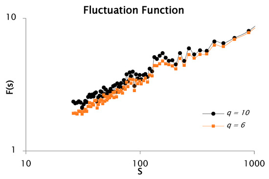
Figure 1.
Log–log representation for the fluctuation function coming from rainfall data with q = 10 and q = 6.
Figure 1 presents the fluctuation function , which reflects the scaling behavior of the signal based on a fixed number of analysis windows. The plot exhibits multiple slope variations and irregular fluctuations, indicating the presence of multiple scaling regimes. Such variations in slope are characteristic of multifractal processes. This behavior is consistent across the examined statistical moments, particularly and , further confirming the multifractal nature of the rainfall time series.
This procedure is systematically applied across multiple temporal scales (segment sizes) of the time series to establish the relationship between the fluctuation function and the segment length , for various values of the statistical moment . Moreover, the slope of the log–log plot of versus corresponds to the generalized Hurst exponent associated with the -order moment, as defined in Equation (14).
The Logarithmic transformation of Equation (15) provides the generalized Hurst exponent for q = 10, as shown in Figure 2.
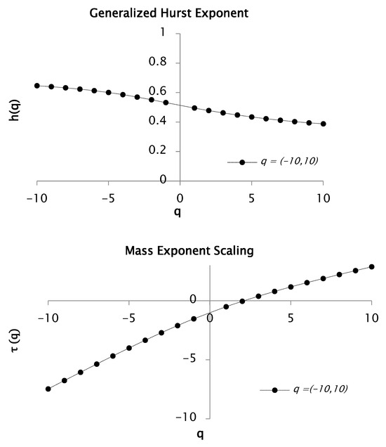
Figure 2.
Function and for values between −10 and 10. This function generates a multifractal spectrum.
Figure 2 provides further evidence that the rainfall time series exhibits multifractal characteristics, as indicated by the pronounced dependence of the mass exponent function on the statistical moment . The asymmetric behavior observed for and reflects distinct variations in the slope of the connecting segments, suggesting differing scaling properties for small and large fluctuations. Based on the relation , the estimated Hurst exponent is 0.38, yielding a corresponding fractal dimension of . For negative values of , the slope of is approximately 0.69, whereas for positive values it is approximately 0.34. Additionally, the convex shape of the curve supports the multifractal nature of the time series.
The multifractal—or singularity—spectrum was derived via Equation (16), which represents the Legendre transform pair used to relate the mass exponent function to the singularity strength and fractal dimension. Figure 3 presents the resulting multifractal spectrum of the rainfall time series for statistical moment values and .
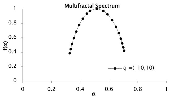
Figure 3.
Multifractal spectrum of rainfall series recorded between 1951 and 2001. was obtained from functions and for values of q from −10 to 10.
The multifractal spectrum displayed in Figure 3 exhibits a concave shape, indicative of a heterogeneous structure composed of regions characterized by distinct Hölder exponents . This heterogeneity gives rise to the multifractal spectrum , where the inverse parabolic form of the curve confirms the multifractal nature of the rainfall time series. The width of the spectrum, defined as , quantifies the variability or complexity of the signal. In this study, serves as a direct measure of the degree of multifractality present in the precipitation data. For the analyzed series, the estimated values of and yield a spectral width of , reflecting the range of singularities and underscoring the multifractal strength inherent to the rainfall process.
The presence of a dense clustering of points at both extremes of the multifractal spectrum typically suggests the occurrence of extreme events that deviate substantially from the mean. This behavior is particularly informative when analyzing higher-order moments across a broad range of values. Conversely, an asymmetry in the spectrum, where one branch is noticeably shorter than the other, may reflect a more homogeneous distribution of values within the dataset.
Keeping up with the results, we carried out a similar analysis to the previous moment but with . Multifractal spectrums for values ranging from −6 to 6 were obtained from functions and , proving multifractal behavior in rainfall for this order of moment. The results are shown in Figure 4.
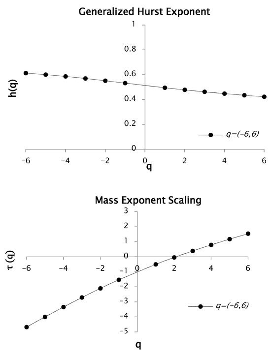
Figure 4.
Function and for values between −6 and 6. This function generates a multifractal spectrum.
Figure 4 illustrates the multifractal behavior of the rainfall time series, evidenced by the marked dependence between the statistical moment and the mass exponent . The asymmetric scaling response for positive and negative values—reflected in the distinct slopes across the curve—demonstrates that small- and large-magnitude fluctuations contribute differently to the overall dynamics. Based on the relationship between the Hurst exponent and the scaling exponent , the Hurst exponent was estimated as 0.38. Consequently, the fractal dimension was calculated as 1.58.
For this case, we obtained a slope of 0.62 with negative values of q, whereas for positive values we obtained 0.38. Curve is also a convex curve, hence, it presents multifractal characteristics.
As previously outlined, the multifractal—or singularity—spectrum was computed using Equation (16), which represents the Legendre transform pair. Figure 5 displays the resulting multifractal spectrum for the rainfall time series corresponding to q values of −6 and 6.
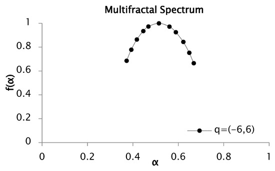
Figure 5.
Multifractal spectrum of rainfall series recorded between 1951 and 2001 for values of between −6 and 6.
The spectrum illustrated in Figure 5 exhibits a maximum singularity strength of 0.67 and a minimum value of 0.36, yielding a spectral width of 0.29.
In this case, the multifractal spectra presented in Figure 3 and Figure 5 exhibit a relatively symmetric shape, with comparable lengths of the left and right branches, indicating a homogeneous distribution of singularity strengths and their corresponding fractal dimensions .
Moreover, a multifractal analysis of the previous time series is presented with the difference that, in this analysis, the number of segments or windows is down to 50, but with the same statistical moments for as the previous analysis. Following the application of Equation (9) to construct the cumulative profile of the rainfall series, a subsequent fluctuation function analysis was performed for and , utilizing window sizes of 50 segments, as illustrated in Figure 6.
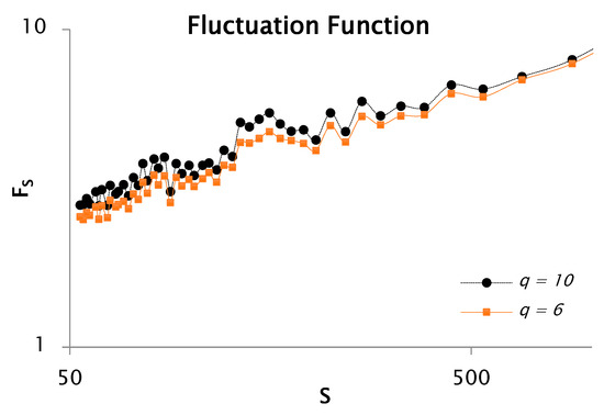
Figure 6.
Log–log representation for the function of rainfall data fluctuation for 10 and 6, with 50 segments or windows.
Figure 6 represents the evolution of the fluctuation function when analyzing only 50 segments or windows. The figure also reveals notable variations and slope transitions in the fluctuation function for both and , indicative of scale-dependent behavior. By contrasting the fluctuation functions showed in Figure 1 and Figure 6, it can be noticed that, in the latter, the fluctuation function presents less oscillations due to less analyzed windows. Hence, we obtained a better (intermittency of the discretize) signal. As mentioned in the previous analysis, changes in slope are signals of multiple scaling, (i.e., multifractal nature). This pattern is highly consistent across both analyzed moments, and . Moreover, the slope of the fluctuation function corresponds to the generalized Hurst exponent associated with each moment order. Figure 7 shows that the rainfall time series has clear multifractal characteristics, as reflected in the strong dependence between the generalized exponent and . The analysis resulted in a Hurst exponent of 0.38 and a corresponding fractal dimension of 1.6. The slope was estimated to be 0.69 for negative values of and 0.35 for positive values. In addition, the convex profile of the curve further proves the multifractal behavior of the dataset.
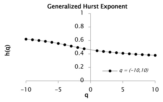
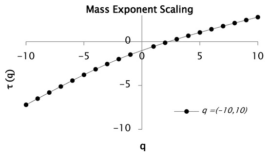
Figure 7.
Function and for values between and with 50 segments or windows.
Figure 8 displays the multifractal spectrum of the rainfall time series computed over a full range of moment orders, with q varying from −10 to 10.
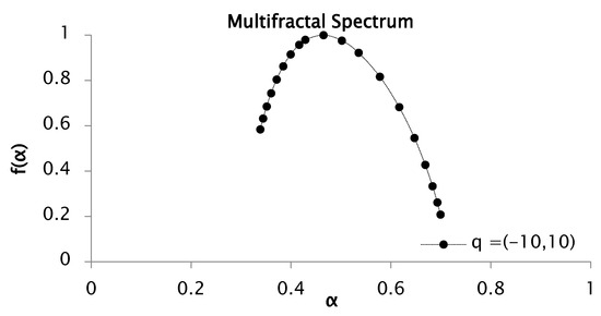
Figure 8.
Multifractal spectrum of rainfall series recorded between 1951 and 2001, for values of between −10 to 10, with 50 segments or windows.
The multifractal spectrum depicted in Figure 8 exhibits a concave profile, with distinct segments of the structure characterized by varying Hölder exponents , thereby confirming the multifractal nature of the signal through the corresponding distribution. In this study, the spectrum width was computed for the rainfall time series, yielding and . Consequently, the spectral width was estimated as , which reflects the range of fluctuation intensities present in the dataset.
This multifractal spectrum shows the right branch to be longer than the one on the left. This is an indicator of great heterogeneity between the values of the rainfall series.
Keeping up with the results, we carried out a similar analysis as the previous moment 10 but with 6. Multifractal spectrums for values ranging from −6 to 6 were obtained from functions , and . The results are shown in Figure 9.
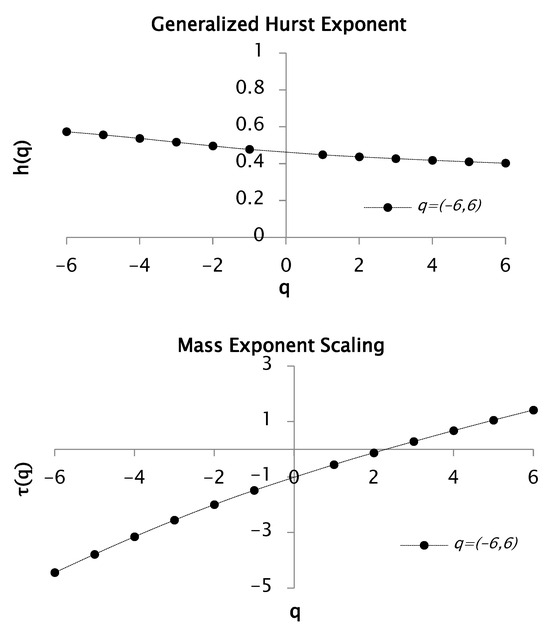
Figure 9.
Functions and for values between −6 and 6 with 50 segments or windows. This function generates a multifractal spectrum.
In Figure 9 the multifractal nature of the rainfall time series is proved, with a Hurst exponent of 0.40 and a fractal dimension of 1.60. The convexity of the curve further supports this behavior. Additionally, a concave spectrum with notable heterogeneity is revealed in Figure 10.
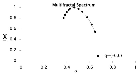
Figure 10.
Multifractal spectrum of rainfall series recorded between 1951 and 2001 for values of from −6 to 6 with 50 segments or windows.
The multifractal spectrum shown in Figure 10 is concave, with and , resulting in a spectrum width of . The asymmetry of the spectrum, with a broader right branch, reflects significant heterogeneity in the rainfall data.
3.2. Multifractal Analysis of Precipitation Series by Decades
The decades considered for the multifractal analysis were from 1951 to 2001.
As previously stated, the objective was to derive the singularity spectrum to verify the presence of multifractal scaling behavior in the decadal precipitation time series and to examine how the characteristics of one series vary relative to another. Therefore, the statistical moment “.” was required to be defined. As an example, it was between −10 and 10. For a and applying Equation (9, the profile of the series was determined. Now, with this defined profile, the fluctuation analysis was conducted for as shown in Figure 11. This procedure was conducted in the same way for a moment . It is necessary to highlight that in this case the fluctuation analysis was given from 100 segments or windows. Subsequently, another analysis was introduced for 50 segments, for the moments and .
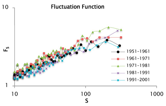
Figure 11.
Log–log plot for the fluctuation function by decades of precipitation data taking a and 100 segments or windows.
As previously noted, the variations in the slope of the fluctuation functions across decades provide evidence of multiple scaling behavior, thereby confirming the multifractal nature of the signal in each analyzed period. Accordingly, the slope of the fluctuation function represents the generalized Hurst exponent associated with the moment of order , denoted as .
If we take logarithms on both sides of Equation (15 we obtain the graph of the Hurst exponent generalized for values of , in this case between −10 and 10. The results can be seen in Figure 12, where the functions and for each of the decades are shown.
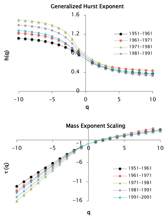
Figure 12.
and functions for values of between −10 and 10 per decades of precipitation data taking a value of 100 segments or windows.
Figure 12 illustrates that the decadal precipitation time series exhibits multifractal characteristics, as evidenced by the pronounced dependence between the generalized moment order and the scaling exponent . Distinct behaviors are observed for negative and positive values of , reflected in the variation in the slope connecting the respective data points. Based on the relationship between the generalized Hurst exponent and the classical Hurst exponent , the Hurst exponent was estimated for each decade. Subsequently, the fractal dimension was derived using the expression . These results are summarized in Table 1.

Table 1.
Values of the Hurst exponent and fractal dimension for a time and 100 segments or windows.
The previous table shows the values of the Hurst exponent and the fractal dimension by decades, taking 100 windows as a partition of the support set and a . Remarkably, similar values were found for the following decades: [1951–1961], [1971–1981], [1981–1991] and [1991–2001]. For the [1961–1971] decade there is a slightly higher value. On the other hand, the exponent values are less than 0.5, which allows us to infer that the precipitation series shows anti-persistence. Therefore, if in a small time range the precipitation increases, there is a high probability that in the following time range the precipitation will decrease.
In Figure 12, for negative values of there are slopes, and for positive values, there are also slopes. Therefore, the curves are convex, indicating the presence of multifractal characteristics. It can also be noticed that the curves corresponding to the precipitation series over the decades are overlapped for values of . Nonetheless, for values there is a different situation that can be explained with the help of multifractal spectra.
Again, using Equation (16), corresponding to the pair of Legendre transformations, the multifractal or singularity spectra were determined. In Figure 13, the multifractal spectrum of precipitation can be seen for values of between −10 and 10.
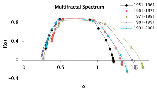
Figure 13.
Multifractal spectrum of the precipitation series recorded by decades, from the and functions for values of from −10 to 10, and 100 segments or windows.
Figure 13 displays a concave multifractal spectrum, consistent with the presence of multifractality in the precipitation time series. The various segments of the curve are defined by distinct Hölder exponent values , which collectively give rise to the singularity spectrum . The values are associated with the variation coefficient of the precipitation series. In this analysis, was estimated for the precipitation data series whose values are reported in Table 2. The range or width of the multifractal spectrum can be seen in this table, it increases in order of the series [1951–1961] < [1961–1971] < [1991–2001] < [1981–1991] < [1971–1981]. The values represent the range between the maximum and minimum precipitation values. The series for the years [1971–1981] have the maximum value of , indicating greater variability in the precipitations for this decade. On the other hand, the above spectra have a longer right branch than the left one, which indicates a great heterogeneity between the precipitation values of the series. When a branch of a spectrum is overlapped with respect to another multifractal spectrum, it indicates similarity in the data. As an example, there are the spectra of the series of [1951–1961], [1971–1981], and [1981–1991]; the left branches of these spectra are overlapped, therefore the first years of these decades show similarities in the behavior of the precipitations.
Table 2.
Values of and to obtain the width of the multifractal spectrum for and 100 segments or windows.
Now, the previous analysis was conducted for a moment . Just as in the previous case, the analysis of fluctuations was given from 100 segments or windows. The behavior of the series was very similar to Figure 11, therefore the results were shown directly for .
From Equation (15), the graph of the Hurst exponent, generalized for values of , was obtained, in this case between −6 and 6. The results are observed in Figure 14, where the functions and are shown for each of the decades.
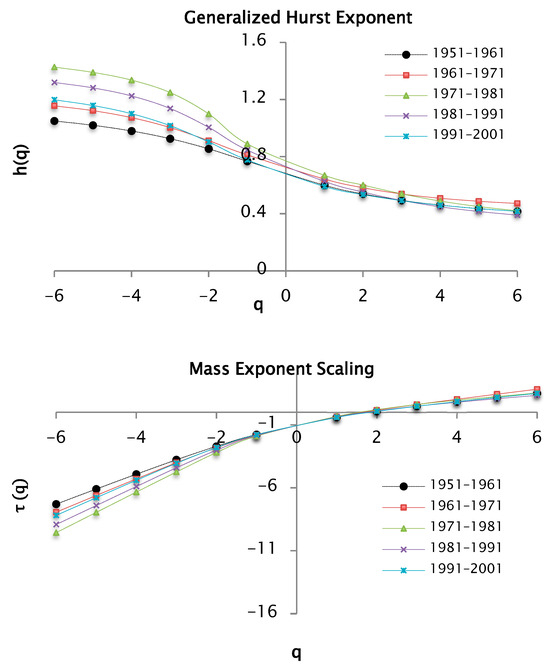
Figure 14.
and functions for values of between −6 and 6 for decades of precipitation data taking a value of 100 segments or windows.
The multifractal behavior of the precipitation series is shown in Figure 14 and the results in Table 3.
Table 3.
Values of the Hurst exponent and fractal dimension for a moment 6 and 100 segments or windows.
Table 3 shows the values of the Hurst exponent and the fractal dimension by decade, taking 100 windows as a partition of the support set and a . As for the analysis of , similar values were maintained for the following decades: [1951–1961], [1971–1981] and [1991–2001]. For the [1981–1991] decade, there is a value of 0.39, and for 1961–1971, there is a value of 0.47. Compared to Table 1, the values for increased. In this case, the exponent values were also less than 0.5, allowing us to infer that the precipitation series shows anti-persistence character. Thus, convex curves can be seen in Figure 14, which indicates multifractal behavior. For , the curves overlap, while for , there are some differences, explained by the multifractal spectrum from Figure 15.
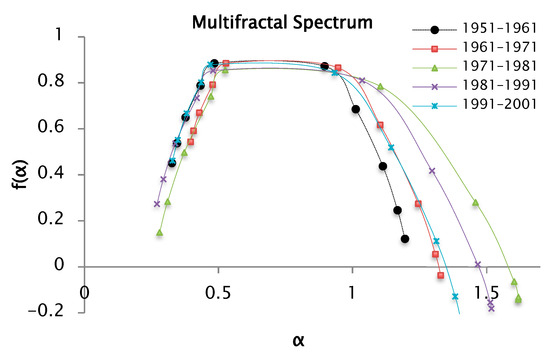
Figure 15.
Multifractal spectrum of the precipitation series recorded by decades, from the and functions for values of from −6 to 6 and 100 segments or windows.
The multifractal spectrum shown in Figure 15 is also a concave function like the other introduced spectra. The distinct parts of the structure are characterized by different values of , leading to the existence of the multifractal spectrum . The values are associated with the coefficient of variation in the precipitation series. In this analysis, was estimated for the precipitation data series and these values are reported in Table 4, in which the range or width of the multifractal spectrum can be seen. It increases in order of the series [1951–1961] < [1961–1971] < [1991–2001] < [1981–1991] < [1971–1981]. This behavior is like the analysis for a . The values represent the range between the maximum and minimum precipitation values. The series from [1971–1981] have the maximum value of , which indicates a greater variability in the precipitations that correspond to this decade.
Table 4.
Values of and to obtain the width of the multifractal spectrum for and 100 segments or windows.
Finally, making a comparative analysis between the widths corresponding to the multifractal spectra for and , it can be seen that increases as the moment is greater.
We introduce a similar analysis below for the same moments and , with the difference that in this case 50 segments are used to divide the support set.
Previously, it has been shown that the functions and corresponding to the precipitation series by decades have multifractal behavior. These results are shown in Figure 16.
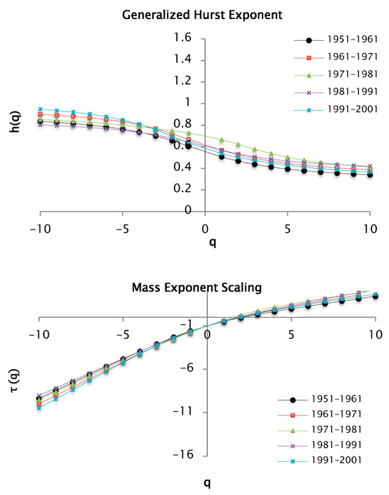
Figure 16.
Functions and for values of for decades of precipitation data taking a value of 50 segments or windows.
The Hurst exponent and fractal dimension by decade are shown in Table 5.
Table 5.
Values of the Hurst exponent and fractal dimension for a moment q = 10 and 50 segments or windows.
Table 5 shows the values of the Hurst exponent and the fractal dimension by decades, taking 50 windows as a partition of the support set and a . The values of the Hurst exponent are slightly variable between the series under study, and are less than 0.5, allowing us to infer that the precipitation series show anti-persistence.
The multifractal spectra of precipitation for values of from −10 to 10 is shown in Figure 17.
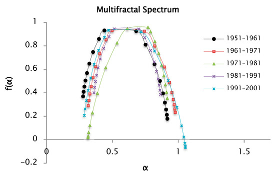
Figure 17.
Multifractal spectrum of the series of precipitations recorded by decades, from the and functions for values of from −10 to 10 and 50 segments or windows.
The multifractal spectrum introduced in Figure 17 is also a concave function like the other presented spectra. The different parts of the structure are characterized by different values of , leading to the existence of the multifractal spectrum ; the values are associated with the coefficient of variation in the precipitation series. In this analysis, is estimated for the precipitation data series. These values are reported in Table 6 where the range or width of the multifractal spectrum can be seen. It increases in order of series [1981–1991] < [1951–1961] < [1991–2001]. The series of [1961–1971] and [1971–1981] show similar values. It is important to highlight that in estimations with fluctuation analysis from fifty segments or windows, values of are lower than those obtained in the analysis with 100 windows. Therefore, in this case, the variability of the precipitation at this scale is lower.
Table 6.
Values of and to determine the width of the multifractal spectrum for 10 and 50 segments or windows.
The series of the years [1991–2001] have the maximum value of . This indicates a greater variability in the precipitations corresponding to this decade. The right branch of the spectrum is longer, which indicates heterogeneity, and the overlapping branches, such as for 1951–1961 and 1981–1991, suggest similar precipitation behavior.
Another important aspect to mention is the accumulation of points at the extremes of the spectrum, when it is more pronounced it indicates the existence of extreme values far from the mean. This behavior can be seen in the left branches, corresponding to the series of 1961–1971 and 1991–2001.
Finally, the analysis for the moment is introduced, remembering that 50 segments are used to divide the support set.
According to Equation (15), the generalized Hurst exponent was computed for values of ranging from −6 to 6. The resulting scaling behavior is illustrated in Figure 18.
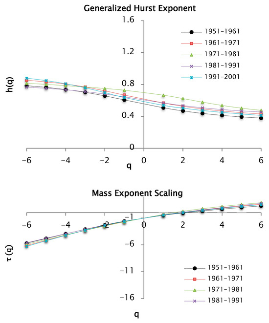
Figure 18.
h(q) and τ(q) functions for q = −6 and q = 6, calculated from decadal precipitation data using 50 segments (or windows).
The values of the Hurst exponent and the fractal dimension by decades are shown in Table 7, considering 50 windows as a partition of the support set, and a . The values of the Hurst exponent are slightly variable between the series under study, and are less than 0.5, which allows us to infer that the precipitation series show anti-persistence character.
Table 7.
Values of the Hurst exponent and fractal dimension for a moment and 50 segments or windows.
The multifractal spectra of precipitation for q values of −6 and 6 are shown in Figure 19.
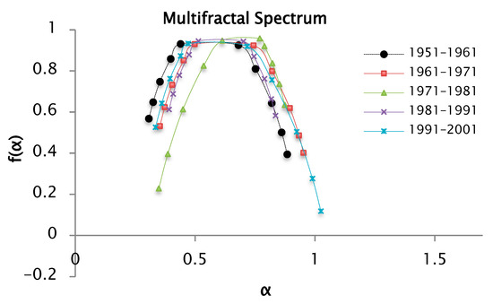
Figure 19.
Multifractal spectrum f(α) of precipitation data by decades, based on h(q) and τ(q) functions for q = −6 and q = 6, with 50 segments.
The multifractal spectrum introduced in Figure 19 is also a concave function like the other introduced spectra. The different parts of the structure are characterized by different values of , leading to the existence of the multifractal spectrum . The values are associated with the coefficient of variation in the precipitation series. In this analysis is also estimated for the precipitation data series. These values are reported in Table 8. In this table the range or width of the multifractal spectrum can be seen, increases in order of series [1981–1991] < [1971–1981] < [1951–1961] < [1961–1971] < [1991–2001]. It is important to highlight that in estimations with fluctuation analysis from 50 segments or windows, values are lower than those obtained in the analysis from 100 segments or windows.
Table 8.
Values of and to obtain the width of the multifractal spectrum for and 50 segments or windows.
The series of the years [1991–2001] continued to have the maximum value of , indicating a greater variability in the precipitations corresponding to this decade. On the other hand, the multifractal spectra had a similar behavior to the analysis for a , where the branch on the right kept being longer than the one on the left, indicating a great heterogeneity between the precipitation values of the series. When a branch of a spectrum overlapped with respect to that of another multifractal spectrum, it indicated similarity in the data. The branches on the right in the multifractal spectra of the series corresponding to [1951–1961] and [1981–1991] were overlapped, therefore there are similarities in the behavior of the precipitations.
In the previous analysis for a , there is no accumulation of points at the ends of the multifractal spectra, contrary to the case for a and with the same resolution in the partition of the support set.
Finally, making a comparative analysis between corresponding to the multifractal spectra for a and , and considering the obtaining of the fluctuation function from a number of windows or segments equal to 100 and 50; it was found that increases as the moment is greater than and the analysis of windows is greater.
Following [31], the adjustment of the experimental multifractal spectra could be carried out, in this case for moments of order . The binomial spectrum was used as a theoretical spectrum, given a probability , a resolution , and moments , defined by the following pair of parametric equations:
and
The binomial spectra used were transformed as and , where and are two adjustment factors. The theoretical and experimental graphs are compared in Figure 20, Figure 21, Figure 22, Figure 23 and Figure 24, corresponding to the decades [1981–1991], [1991–2001], [1951–1961], [1961–1971] and [1971–1981], respectively. The values of , , , and , as well as the fractal dimensions of the support and information , respectively, are presented in the figures. The good agreement between the equivalent and experimental binomial spectra was clearly demonstrated.
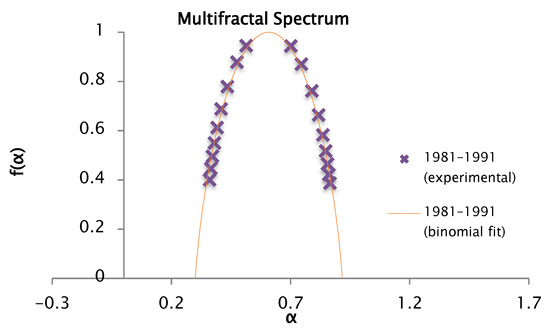
Figure 20.
Comparison of the experimental and binomial spectra for the values of , , and . With fractal dimension and information 0.90.
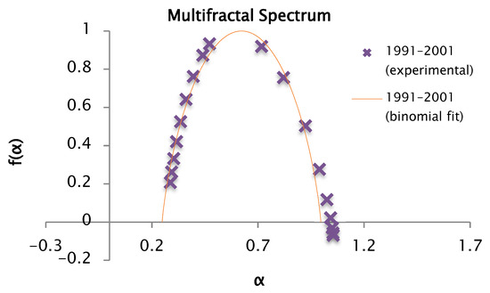
Figure 21.
Comparison of the experimental and binomial spectra for the values of , , and , with fractal dimension and information 0.85.
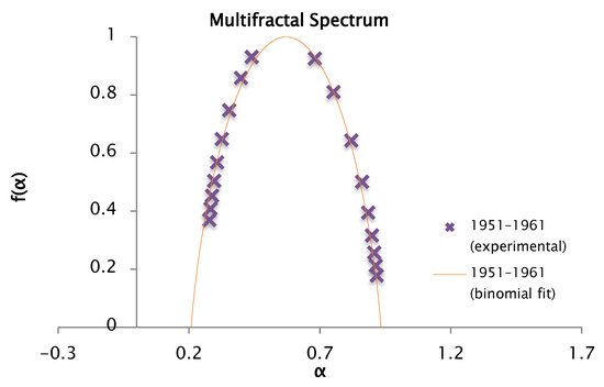
Figure 22.
Comparison of the experimental and binomial spectra for the values of , , and , with fractal dimension and information 0.83.
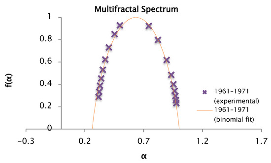
Figure 23.
Comparison of the experimental and binomial spectra for the values of , , and , with fractal dimension and information 0.86.
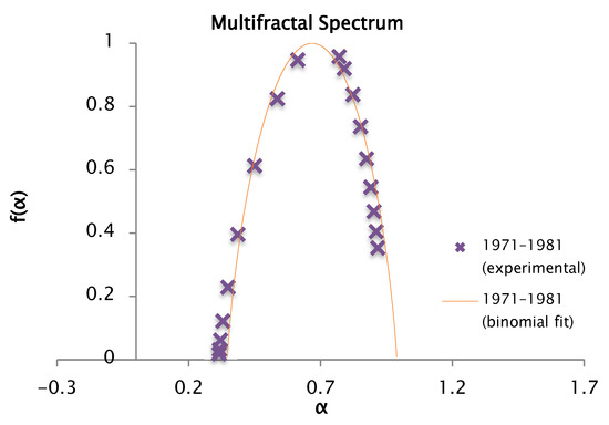
Figure 24.
Comparison of the experimental and binomial spectra for the values of , , and , with fractal dimension and information 0.91.
The theoretical mean and the experimental mean graphs are compared in Figure 25 corresponding to the average of the decades [1951–1961], [1961–1971], [1971–1981], [1981–1991] and [1991–2001], respectively. The figures show the values of , , , and , as well as the fractal dimensions of the support and information , respectively.
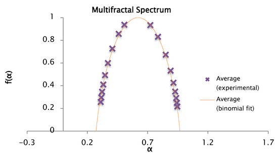
Figure 25.
Comparison of the experimental and binomial spectra for the values of , , and , with fractal dimension and information 0.87.
4. Conclusions
The present study confirmed the multifractal characteristics of daily precipitation time series through the application of the Multifractal Detrended Fluctuation Analysis (MFDFA) method. This approach enabled the extraction of key multifractal complexity parameters, namely and , and facilitated the construction of multifractal spectra based on observations from a single climatological monitoring station.
Furthermore, the estimation of the generalized Hurst exponent allowed for the characterization of the precipitation time series in terms of its temporal dynamics, distinguishing persistent, anti-persistent, and stochastic behaviors across different scales.
Secondly, the application of the Multifractal Detrended Fluctuation (MFDFA) further validated the multifractal nature of the precipitation time series. The pronounced linear relationship between versus , together with the consistent shapes of the resulting multifractal spectra, supports the suitability of the data for multifractal interpretation. Moreover, the strong dependence between the moment order and the scaling mass exponent confirms the multifractal behavior of the signal. Distinct responses for and reflect asymmetries in the slope connecting both regions, indicative of structural heterogeneity. The derived multifractal spectra also enabled the accurate estimation of the fractal dimension of the support set and the information dimension, providing further quantitative insight into the complexity of the precipitation process.
The value of the Hurts exponent of a synthetic monthly series is like that obtained from the observed monthly data. Similarly, the fractal analysis of precipitation at the considered climatic station allows us to conclude that
The preliminary results show that the series under study are persistent (i.e., there is a high probability that precipitation will increase in a time range immediately after a range where a decrease is observed).
The fractal dimension of the precipitation series is close to the unit, indicating that it is a signal of limited and highly persistent variation. The information dimension of less than the unit indicates that the subset where the measurement is concentrated is not equal to the interval of variation in the same.
Regarding multifractal analysis, it has been shown to be an adequate and efficient tool to characterize precipitation series. The multifractal spectra derived from the Centenario Dam climatological station exhibit pronounced asymmetry, with extended right-hand branches in most cases. This pattern reflects substantial heterogeneity in the temporal distribution of precipitation.
In some multifractal analyses conducted by decades, the spectrum presents values less than zero, which are not a product of the characteristics of the series itself, but of numerical instabilities due to divergence of the moments, given the proximity to zero.
The experimental multifractal spectra were well fitted with a theoretical binomial spectrum, which has allowed the estimation of the fractal dimension of the precipitation support set while maintaining a good precision in the calculation of the information dimension
Consequently, due to the similarity of the different multifractal spectra obtained for each of the five decades of precipitation observations, the precipitation can be estimated at different time scales with an average multifractal spectrum. Therefore, the application of multifractal theory is encouraged in future studies, as it offers a robust mathematical framework to explore scale invariance and to characterize the behavior of climatic variables through scaling laws defined by their associated exponents.
Finally, this study enhances the understanding of hydroclimatic dynamics in the Semi-Arid Central Mexican Plateau and provides a scientific basis for developing precipitation forecasting models. Such predictive tools are essential for designing climate change adaptation strategies, particularly in regions vulnerable to drought and water scarcity. Future research could focus on integrating multifractal analysis with climate models and remote sensing data to improve both spatial resolution and predictive accuracy. Applying these methods to short- and medium-term precipitation forecasting under various climate scenarios, and conducting comparative studies across regions and time scales, could inform early warning systems and strengthen evidence-based water resource planning. These advances support the goals of Sustainable Development Goal 13 (Climate Action).
Author Contributions
Conceptualization, A.A.L.-L., C.F. and A.L.-R.; methodology, A.A.L.-L. and Y.S.-U.; software, A.A.L.-L.; validation, C.F. and A.L.-R.; formal analysis, A.A.L.-L.; investigation, A.A.L.-L. and C.F.; resources, A.A.L.-L. and N.M.G.T.; data curation, C.F.; writing—original draft preparation, A.A.L.-L.; writing—review and editing, Y.S.-U.; visualization, A.A.L.-L. and A.L.-R.; supervision, C.F.; project administration, A.L.-R.; funding acquisition, A.A.L.-L. and N.M.G.T. All authors have read and agreed to the published version of the manuscript.
Funding
This research was funded by HIDRUS S.A. de C.V. and Grupo HIDRUS S.A.S. The APC was funded by HIDRUS S.A. de C.V., Grupo HIDRUS S.A.S and Universidad Pontificia Bolivariana Campus Montería. The funders had no roles in the design of the study; in the collection, analysis, or interpretation of data; in the writing of the manuscript, or in the decision to publish the articles. The paper reflects the views of the scientists and not those of the funders.
Institutional Review Board Statement
Not applicable.
Informed Consent Statement
Not applicable.
Data Availability Statement
The data presented in this study are available on request from the corresponding author. The data are not publicly available due to privacy restrictions.
Conflicts of Interest
Author Alvaro Alberto López-Lambraño was employed by the company Hidrus S.A. de C.V. and Grupo Hidrus S.A.S. The remaining authors declare that the research was conducted in the absence of any commercial or financial relationships that could be construed as a potential conflict of interest.
References
- Gao, C.; Guan, X.; Booij, M.J.; Meng, Y.; Xu, Y.-P. A New Framework for a Multi-Site Stochastic Daily Rainfall Model: Coupling a Univariate Markov Chain Model with a Multi-Site Rainfall Event Model. J. Hydrol. 2021, 598, 126478. [Google Scholar] [CrossRef]
- Nguyen, T.H.T.; Bennett, B.; Leonard, M. Evaluating Stochastic Rainfall Models for Hydrological Modelling. J. Hydrol. 2023, 627, 130381. [Google Scholar] [CrossRef]
- Zheng, W.; Zhou, X.; Wang, H.; Luo, J.; Kou, B.; Tang, Z. Integrated Hydrological Model Based on Undirected MDPM: A Case Study of Rainfall Process Simulation for Mountain Highways. J. Hydrol. 2025, 660, 133130. [Google Scholar] [CrossRef]
- Martínez-Acosta, L.; Medrano-Barboza, J.P.; López-Ramos, Á.; Remolina López, J.F.; López-Lambraño, Á.A. SARIMA Approach to Generating Synthetic Monthly Rainfall in the Sinú River Watershed in Colombia. Atmosphere 2020, 11, 602. [Google Scholar] [CrossRef]
- Adarsh, S.; Nourani, V.; Archana, D.S.; Dharan, D.S. Multifractal Description of Daily Rainfall Fields over India. J. Hydrol. 2020, 586, 124913. [Google Scholar] [CrossRef]
- da Silva, A.S.A.; Stosic, T.; Arsenić, I.; Menezes, R.S.C.; Stosic, B. Multifractal Analysis of Standardized Precipitation Index in Northeast Brazil. Chaos Solitons Fractals 2023, 172, 113600. [Google Scholar] [CrossRef]
- Gómez-Gómez, J.; Plocoste, T.; Alexis, E.; Jiménez-Hornero, F.J.; de Ravé, E.G.; Nuiro, S.P. Multifractal Detrended Fluctuation Analysis of Rainfall Time Series in the Guadeloupe Archipelago. J. Hydrol. 2023, 626, 130377. [Google Scholar] [CrossRef]
- Sarker, A.; Mali, P. Detrended Multifractal Characterization of Indian Rainfall Records. Chaos Solitons Fractals 2021, 151, 111297. [Google Scholar] [CrossRef]
- Langousis, A.; Veneziano, D.; Furcolo, P.; Lepore, C. Multifractal Rainfall Extremes: Theoretical Analysis and Practical Estimation. Chaos Solitons Fractals 2009, 39, 1182–1194. [Google Scholar] [CrossRef]
- Monjo, R.; Locatelli, L.; Milligan, J.; Torres, L.; Velasco, M.; Gaitán, E.; Pórtoles, J.; Redolat, D.; Russo, B.; Ribalaygua, J. Estimation of Future Extreme Rainfall in Barcelona (Spain) under Monofractal Hypothesis. Int. J. Climatol. 2023, 43, 4047–4068. [Google Scholar] [CrossRef]
- Kantelhardt, J.W.; Zschiegner, S.A.; Koscielny-Bunde, E.; Havlin, S.; Bunde, A.; Stanley, H.E. Multifractal Detrended Fluctuation Analysis of Nonstationary Time Series. Phys. A Stat. Mech. Its Appl. 2002, 316, 87–114. [Google Scholar] [CrossRef]
- Mandelbrot, B.B. The Fractal Geometry of Nature; Freeman: San Francisco, CA, USA, 1982. [Google Scholar]
- Serinaldi, F. Use and Misuse of Some Hurst Parameter Estimators Applied to Stationary and Non-Stationary Financial Time Series. Phys. A Stat. Mech. Its Appl. 2010, 389, 2770–2781. [Google Scholar] [CrossRef]
- Wolfensberger, D.; Gires, A.; Tchiguirinskaia, I.; Schertzer, D.; Berne, A. Multifractal Evaluation of Simulated Precipitation Intensities from the COSMO NWP Model. Atmos. Chem. Phys. 2017, 17, 14253–14273. [Google Scholar] [CrossRef]
- Vahab, S.; Sankaran, A. Multifractal Applications in Hydro-Climatology: A Comprehensive Review of Modern Methods. Fractal Fract. 2025, 9, 27. [Google Scholar] [CrossRef]
- Lovejoy, S.; Schertzer, D. The Weather and Climate: Emergent Laws and Multifractal Cascades; Cambridge University Press: Cambridge, UK, 2013; pp. 113–175. [Google Scholar] [CrossRef]
- Intergovernmental Panel on Climate Change (IPCC). Climate Change 2022: Impacts, Adaptation and Vulnerability. Sixth Assessment Report. Available online: https://www.ipcc.ch/report/ar6/wg2/ (accessed on 10 December 2024).
- Campbell, B.M.; Hansen, J.; Rioux, J.; Stirling, C.M.; Twomlow, S.; Wollenberg, E. Urgent Action to Combat Climate Change and Its Impacts (SDG 13): Transforming Agriculture and Food Systems. Curr. Opin. Environ. Sustain. 2018, 34, 13–20. [Google Scholar] [CrossRef]
- Yong, Y.; Ahmed, Z.; Wang, S.; Rjoub, H.; Bilan, Y. Minerals, Natural Resources, Government Instability, and Growing Ecological Challenges: Can We Achieve SDGs 12 and 13? Resour. Policy 2024, 88, 104507. [Google Scholar] [CrossRef]
- Sherif, M.; Abrar, M.; Baig, F.; Kabeer, S. Gulf Cooperation Council Countries’ Water and Climate Research to Strengthen UN’s SDGs 6 and 13. Heliyon 2023, 9, e14584. [Google Scholar] [CrossRef]
- Achour, R.; Li, Z.; Selmi, B.; Wang, T. A Multifractal Formalism for New General Fractal Measures. Chaos Solitons Fractals 2024, 181, 114655. [Google Scholar] [CrossRef]
- Halsey, T.C.; Jensen, M.H.; Kadanoff, L.P.; Procaccia, I.; Shraiman, B.I. Fractal Measures and Their Singularities: The Characterization of Strange Sets. Phys. Rev. A 1986, 33, 1141. [Google Scholar] [CrossRef]
- Frisch, U.; Parisi, G. On the Singularity Structure of Fully Developed Turbulence. In Turbulence and Predictability in Geophysical Fluid Dynamics and Climate Dynamics; North-Holland: Amsterdam, The Netherlands, 1985; pp. 84–88. [Google Scholar]
- Leonarduzzi, R.; Touchette, H.; Wendt, H.; Abry, P.; Jaffard, S. Generalized Legendre Transform Multifractal Formalism for Nonconcave Spectrum Estimation. In Proceedings of the 2016 IEEE Statistical Signal Processing Workshop (SSP), Palma de Mallorca, Spain, 26–29 June 2016; p. 5. [Google Scholar] [CrossRef]
- Emmanouil, S.; Langousis, A.; Nikolopoulos, E.I.; Anagnostou, E.N. The Spatiotemporal Evolution of Rainfall Extremes in a Changing Climate: A CONUS-Wide Assessment Based on Multifractal Scaling Arguments. Earth’s Future 2022, 10, e2021EF002539. [Google Scholar] [CrossRef]
- Gómez-Gómez, J.; Ariza-Villaverde, A.B.; Gutiérrez De Ravé, E.; Jiménez-Hornero, F.J. Relationships between Reference Evapotranspiration and Meteorological Variables in the Middle Zone of the Guadalquivir River Valley Explained by Multifractal Detrended Cross-Correlation Analysis. Fractal Fract 2023, 7, 54. [Google Scholar] [CrossRef]
- Baranowski, P.; Krzyszczak, J.; Slawinski, C.; Hoffmann, H.; Kozyra, J.; Nieróbca, A.; Siwek, K.; Gluza, A. Multifractal Analysis of Meteorological Time Series to Assess Climate Impacts. Clim. Res. 2015, 65, 39–52. [Google Scholar] [CrossRef]
- Stosic, B.; Stosic, T.; Tošić, I.; Djurdjević, V. Multifractal Analysis of Temperature in Europe: Climate Change Effect. Chaos Solitons Fractals 2025, 196, 116386. [Google Scholar] [CrossRef]
- López Lambraño, A. Análisis Multifractal y Modelación de La Precipitación. Ph.D. Thesis, Universidad Autónoma de Querétaro, Santiago de Querétaro, Mexico, 2012. [Google Scholar]
- López, A.; Carrillo, E.; Fuentes, C.; López, A.; López, M. Una Revisión de Los Métodos Para Estimar El Exponente de Hurst y La Dimensión Fractal En Series de Precipitación y Temperatura. Rev. Mex. Fis. 2017, 63, 244–267. [Google Scholar]
- Falconer, K. Fractal Geometry Mathematical Foundations and Applications; John Wiley and Sons: Hoboken, NJ, USA, 1990. [Google Scholar]
- Telesca, L.; Colangelo, G.; Lapenna, V.; Macchiato, M. Monofractal and Multifractal Characterization of Geoelectrical Signals Measured in Southern Italy. Chaos Solitons Fractals 2003, 18, 385–399. [Google Scholar] [CrossRef]
- Telesca, L.; Balasco, M.; Colangelo, G.; Lapenna, V.; Macchiato, M. Investigating the Multifractal Properties of Geoelectrical Signals Measured in Southern Italy. Phys. Chem. Earth Parts A/B/C 2004, 29, 295–303. [Google Scholar] [CrossRef]
- Diego, J.M.; Martínez-González, E.; Sanz, J.L.; Mollerach, S.; Martínez, V.J. Partition Function Based Analysis of Cosmic Microwave Background Maps. Mon. Not. R. Astron. Soc. 1999, 306, 427–436. [Google Scholar] [CrossRef]
- Falconer, K. Techniques in Fractal Geometry; John Wiley and Sons: Hoboken, NJ, USA, 1997. [Google Scholar]
- Jaffard, S. Multifractal Formalism for Functions Part I: Results Valid For All Functions. SIAM J. Math. Anal. 1997, 28, 944–970. [Google Scholar] [CrossRef]
- Jaffard, S. Multifractal Formalism for Functions Part II: Self-Similar Functions. SIAM J. Math. Anal. 1997, 28, 971–998. [Google Scholar] [CrossRef]
- Yuval; Broday, D.M. Studying the Time Scale Dependence of Environmental Variables Predictability Using Fractal Analysis. Environ. Sci. Technol. 2010, 44, 4629–4634. [Google Scholar] [CrossRef]
- Sadegh Movahed, M.; Jafari, G.R.; Ghasemi, F.; Rahvar, S.; Reza Rahimi Tabar, M. Multifractal Detrended Fluctuation Analysis of Sunspot Time Series. J. Stat. Mech. Theory Exp. 2006, 2006, P02003. [Google Scholar] [CrossRef]
- López, A.; Fuentes, C.; López Ramos, A.; Mata, J.; López, M. Spatial and Temporal Hurst Exponent Variability of Rainfall Series Based on the Climatological Distribution in a Semiarid Region in Mexico. Atmosfera 2018, 31, 199–219. [Google Scholar] [CrossRef]
- Serpa-Usta, Y.; López-Lambraño, A.A.; Fuentes, C.; Flores, D.-L.; González-Durán, M.; López-Ramos, A. Santa Ana Winds: Multifractal Measures and Singularity Spectrum. Atmosphere 2023, 14, 1751. [Google Scholar] [CrossRef]
- Baranowski, P.; Gos, M.; Krzyszczak, J.; Siwek, K.; Kieliszek, A.; Tkaczyk, P. Multifractality of Meteorological Time Series for Poland on the Base of MERRA-2 Data. Chaos Solitons Fractals 2019, 127, 318–333. [Google Scholar] [CrossRef]
- Krzyszczak, J.; Baranowski, P.; Zubik, M.; Kazandjiev, V.; Georgieva, V.; Sławiński, C.; Siwek, K.; Kozyra, J.; Nieróbca, A. Multifractal Characterization and Comparison of Meteorological Time Series from Two Climatic Zones. Theor. Appl. Clim. 2019, 137, 1811–1824. [Google Scholar] [CrossRef]
Disclaimer/Publisher’s Note: The statements, opinions and data contained in all publications are solely those of the individual author(s) and contributor(s) and not of MDPI and/or the editor(s). MDPI and/or the editor(s) disclaim responsibility for any injury to people or property resulting from any ideas, methods, instructions or products referred to in the content. |
© 2025 by the authors. Licensee MDPI, Basel, Switzerland. This article is an open access article distributed under the terms and conditions of the Creative Commons Attribution (CC BY) license (https://creativecommons.org/licenses/by/4.0/).