Article

Prediction of Atmospheric Bioaerosol Number Concentration Based on PKO–AGA–SVM Fusion Algorithm and Fluorescence Lidar Telemetry

School of Electrical and Information Engineering, North Minzu University, Yinchuan 750021, China
*
Author to whom correspondence should be addressed.
Atmosphere 2025, 16(6), 638; https://doi.org/10.3390/atmos16060638
Submission received: 28 March 2025 / Revised: 13 May 2025 / Accepted: 19 May 2025 / Published: 23 May 2025
(This article belongs to the Section Atmospheric Techniques, Instruments, and Modeling)

Abstract

In order to realize early warning prediction of the distribution characteristics of atmospheric bioaerosol content, this paper proposes using fluorescence lidar as a technical means to establish a prediction model of atmospheric bioaerosol concentration by obtaining the observation data set of bioaerosol concentration, combining it with the data set of atmospheric environmental parameters related to bioaerosol content, and utilizing the fusion algorithm PKO–AGA–SVM. The trained model was then used to predict the atmospheric bioaerosol concentration and compared with the bioaerosol concentration detected by fluorescence lidar to analyze the relative error of the model in predicting the bioaerosol number concentration with different algorithms as well as the bioaerosol number concentration at different pollution levels of atmospheric environmental quality. The experimental results show that the model prediction using the PKO–AGA–SVM fusion algorithm is better than the SVM, AGA–SVM, and PKO–SVM algorithms, with mean relative errors of 25.79, 20.75, 16.93, and 11.57%, respectively. Then, environmental data with different pollution levels were introduced for model prediction experiments, and the results show that the mean relative error of prediction was 12.75% when the air quality was excellent, the mean relative error of prediction was 13.01% when the air quality was good, the mean error of prediction was 10.53% when the air quality was mildly polluted, and the mean error of prediction was 13.72% when the air quality was moderately polluted. When the air quality was heavily polluted, the mean prediction error was 11.83%. The experimental results show that the prediction model has high accuracy and stability under different atmospheric conditions, which can provide a new research approach and technical support for the early warning system of atmospheric bioaerosol concentration.

1. Introduction

The sources of bioaerosols in the air are diverse, such as environmental pollution and human activities such as sewage treatment processes, all of which can lead to the formation of bioaerosols. Bioaerosols contain a variety of biological particles, which are small in size and light in weight. As the particle size of bioaerosols decreases, the air viscosity becomes more pronounced, and the settling speed slows down in the air. They spread everywhere with the flow of air currents in the atmospheric environment, resulting in the diffusion and transmission of pathogenic bioaerosols, which cause impacts on human health. For example, bioaerosols such as bacteria, fungi, viruses, and pollen can cause allergic respiratory diseases when inhaled by humans [1,2,3]. In addition, the content and distribution of bioaerosols in the air are susceptible to variations in the type and level of atmospheric pollution. Compared to unpolluted air, there is an increase in the concentration and type of bioaerosols in polluted air [4,5]. Therefore, real-time monitoring and early warning prediction of bioaerosols in the air, as well as in-depth study of their distribution characteristics, are crucial for the prevention and control of diseases related to bioaerosols.
With the continuous progress and development of human activities, the degree of atmospheric pollution has also increased. Therefore, how to achieve effective early warning and prediction of pollution status is one of the key factors in atmospheric pollution control and governance. As an efficient computational method, the neural network model has a strong nonlinear prediction capability. By analyzing and calculating factors such as atmospheric pollutants and meteorological conditions, it is widely used in early warning and prediction of atmospheric environmental pollution levels. Xiaonan Li et al. [6] developed a backpropagation neural network model based on wavelet denoising to predict bioaerosol concentration, and experimentally validated the model using datasets collected by fixed-point instruments, demonstrating the effectiveness of the backpropagation neural network model in predicting atmospheric bioaerosol concentrations. Gholamreza Goudarzi et al. [7] predicted the total pollen concentration in an urban area by establishing an artificial neural network model, and evaluated the distribution of pollen in the air throughout the city as well as the correlation between pollen concentration and environmental parameters. Therefore, by establishing a prediction model to comprehensively analyze the numerous factors that affect the content of bioaerosols, it is feasible to predict the distribution of bioaerosols for an extended period, providing a scientific basis for the control and management of atmospheric environmental pollution [8,9,10,11,12,13,14].
Given the potential threat of bioaerosols and the urgent need for real-time remote monitoring, the application of artificial intelligence technology to bioaerosol prediction has become a new research solution in the field of remote sensing detection and detection in atmospheric science. In this paper, a prediction model incorporating PKO (pied kingfisher optimizer), AGA (adaptive genetic algorithm), and SVM (support vector machine) is built, and the prediction model is trained by taking the data set of atmospheric environmental parameters as the input and the data set of bioaerosol concentration profiles as the output. During the training process, the support vector machine optimized by PKO–AGA automatically adjusts the relevant parameters so that the prediction model reaches the global search for the optimal solution and improves the prediction model stability. Subsequently, atmospheric bioaerosol concentration prediction was conducted using datasets with air quality levels of excellent, good, mild pollution, moderate pollution, and severe pollution, and the mean relative error was analyzed separately.

2. Establishment of a Prediction Model for the Number Concentration of Atmospheric Bioaerosols

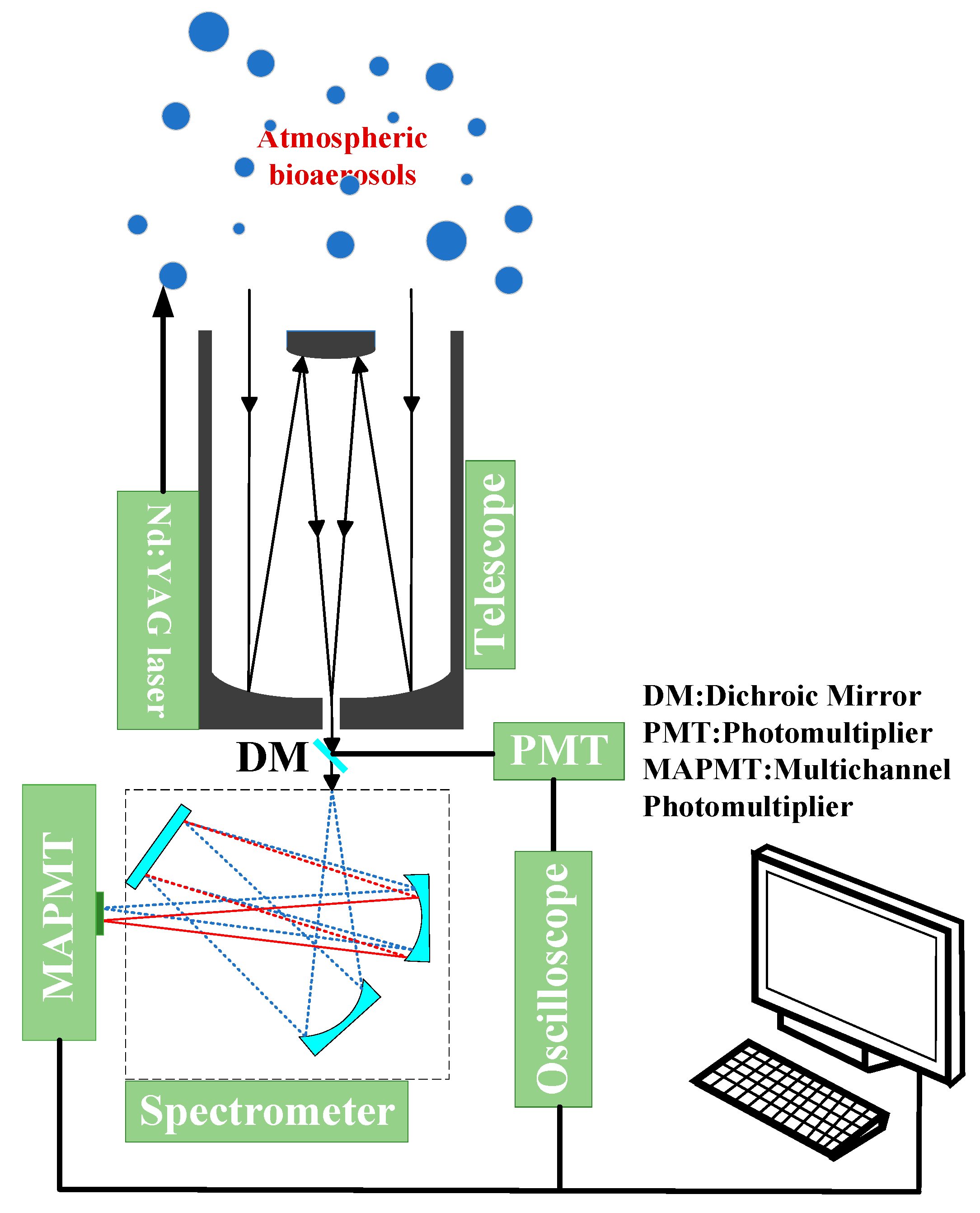
2.1. Bioaerosol Fluorescence Lidar System

Fluorescence lidar detection technology excites biological substances in the atmosphere to produce fluorescence signals by emitting laser pulses of specific wavelengths, and identifies and quantifies target substances by receiving and analyzing these fluorescence signals. Through laser-induced fluorescence, signal reception and processing, and data analysis, we are able to obtain information on the concentration, distribution, and chemical composition of the target substance, thus realizing the detection function [15,16]. Figure 1 shows the basic structure and working principle of atmospheric bioaerosol fluorescence lidar. The fluorescence lidar system uses a digital oscilloscope for data acquisition, and in the process of data acquisition, 11,000 average samples are performed to improve the data stability. The measurement time of each set of data is about 20 min, with a sampling rate of 100 MS/s and an analog bandwidth of 50 MHz. At the same time, the system adopts a 266 nm UV laser pulse as the excitation wavelength of bioaerosol fluorescence, and chooses a 130 nm bandwidth filter to filter and extract the fluorescence signals in the wavelength range of 310 nm–440 nm so that the system’s bioaerosol detection distance can reach 0.8 km.
The power equation for the atmospheric bioaerosol fluorescence lidar echo is shown below.
P ( R ) = 1 2 E 0 η 0 c A 0 R 2 e [ α 1 ( λ 1 , R ) + α 2 ( λ 2 , R ) ] R ξ ( R ) S N B i o ( R )
where P(R) is expressed as the fluorescence signal strength, E0 is the laser pulse output from the laser, c is the speed of light ( m s 1 ), A0 is the receiving area (m2) of the telescope used in the radar system, R is the lidar detection distance (km), α1(λ1,R) is the total extinction coefficient of the excitation wavelength in the atmosphere (km−1), and α2(λ2,R) is the total atmospheric extinction coefficient (km−1) of the fluorescence wavelength. In addition, e [ α 1 ( λ 1 , R ) + α 2 ( λ 2 , R ) ] R in the formula is the transmittance of the excitation and fluorescence wavelengths in the atmosphere. λ1 is the excitation wavelength (nm), λ2 is the fluorescence wavelength (nm), ξ(R) is the geometric overlap factor, S is the effective cross-sectional area for inelastic scattering of the fluorescence, NBio(R) is the concentration of the bioaerosol particles, and η0 is the reception efficiency of the entire optical system for the fluorescence wavelength. The main parameters of the fluorescence lidar system are shown in Table 1.

2.2. PKO–AGA–SVM Fusion Algorithm

2.2.1. Support Vector Machine (SVM)

SVM-based regression estimation approximates any nonlinear function with controllable accuracy, and at the same time, it shows superior performance such as global optimality and good generalization ability [17,18]. Therefore, the application of the support vector machine regression (SVR) algorithm is widely used. For a training sample set (xi, yi), where xiRn is the input vector and yiRn is the output vector, a linear function is fitted to the samples by introducing a nonlinear mapping φ(xi), which realizes the transformation of the sample space to higher dimensions, while for the nonlinear sample, the estimation function f(x) is transformed into the following form:
f ( x ) = W × ϕ ( x ) + b
where W is the weight coefficient, b is the function bias term, and φ(x) is a nonlinear mapping function that serves to map the samples to a higher dimensional space. The introduction of an estimation function in SVM can solve nonlinear regression problems. Assuming that the training samples are fitted linearly with a certain degree of accuracy, and after introducing a relaxation factor into the fitting, the problem of finding the bias term and the weight coefficients is transformed into:
min Q = 1 2 ω 2 + c i = 1 n ( δ i + δ i * )
s . t . y i ω ϕ ( x i ) b ε + δ i * y i + ω ϕ ( x i ) + b ε + δ i * δ i 0 , δ i * 0
where ||ω||2 is used as a descriptive function to react to the complexity of the model, c (cost) is the penalty factor, ε is the fitting error ε > 0, δi and δi* are the relaxation factors, and yi is the output vector. The Lagrange multipliers are introduced in the case of satisfying the constraints, where αi*, αi, υi*, υi ≥ 0. The Lagrange function is defined as:
L = 1 2 ω 2 + C i = 1 n ( δ i + δ i * ) i = 1 n α i ( ω ϕ ( x i ) + b y i + ε + δ i ) i = 1 n α i * ( y i ω ϕ ( x i ) b + ε + δ i * ) i = 1 n ( υ i δ i + υ i * δ i * )
According to the Karush–Kuhn–Tucker (KKT) condition, the partial derivatives of the Lagrange function with respect to the variables ω, b, δi, and δi* are zero. According to duality, the following can be obtained:
ω = i = 1 n ( α i * α i ) x i
The SVM modeling function is:
f ( x ) = i , j = 1 n ( a i a i * ) K ( x i , x j ) + b
b = y i + ε i = 1 n ( α i α i * ) x i
In the model designed in this paper, we chose the radial basis function (RBF) as the kernel function, and its expression is:
K ( x i , x j ) = exp ( | | x i x j | | 2 2 g 2 )
where g (gamma) is the kernel function parameter. The core of SVM is to find the appropriate penalty factor c and the kernel function parameter g to improve the performance of the model. However, manual search often makes the model fall into the local optimal solution, and algorithm optimization can make the results more accurate.

2.2.2. Adaptive Genetic Algorithm (AGA)

The traditional GA with a fixed crossover rate pc and a mutation rate pm shows good robustness in solving general optimal parameters but still has poor stability in dealing with complex problems [19,20]. Therefore, Srinivas et al. [21] proposed a novel algorithm with the name of adaptive genetic algorithm (AGA). AGA could dynamically adjust important parameters such as crossover probability and mutation probability according to the fitness of the population or the characteristics of the problem so as to better explore the solution space, avoid premature or slow convergence, and improve the overall efficiency of the algorithm. Genetic algorithms need to have the ability to converge to an optimal solution after finding the region containing the optimal solution as well as the ability to explore new regions of the solution space when searching for the global optimal solution [22,23]. These two points in the genetic algorithm, on the other hand, are limited to a fixed pc and pm and do not guarantee global convergence of the algorithm. AGA can adaptively change according to the individual fitness, where pc and pm increase as the population falls into the local extreme and decrease as the individuals disperse all over the solution space. The specific calculation process is as follows:
p c = a 1 ( f max f a v g ) f , ( f max f a v g ) f a 2 , ( f max f a v g ) > f
p m = a 3 ( f max f ) f max f a v g , f f a v g a 4 , f < f a v g
In the formula, fmax is the maximum fitness of the population, favg is the mean fitness of the population, f’ is the fitness of the individual with greater fitness on both sides of the crossover process, f is the individual fitness, and a1, a2, a3, and a4 ≤ 0 are constant values.

2.2.3. Pied Kingfisher Optimizer

The pied kingfisher optimizer is inspired by the spotted kingfisher’s perching, hovering, and diving, and its unique symbiotic relationship with the Eurasian otter [24].
The algorithm is implemented as follows:
(1) The pied kingfisher optimizer is similar to other population algorithms, initiating the search process by randomly generating a set of initial solutions in the search space:
X i j = l b + ( u b l b ) × R i = 1 , 2 , , N j = 1 , 2 , , D I M
i = 1 , 2 , , N ; j = 1 , 2 , , D I M ;
where Xi,j denotes the position of the ith individual in the jth dimension; ub and lb denote the upper and lower bounds of the search range, respectively; R denotes a random value of 0–1; N is the total number of scales; and DIM is the total number of dimensions of the currently considered problem. After the first initial population is generated, the fitness function is used to evaluate the ability of each individual, and individuals with higher fitness values are selected to construct a new generation.
(2) Candidate solutions are generated by setting the objective function value based on a random factor R. When R < 0.8, the algorithm enters the exploration phase, which is inspired by the perching and hovering behaviors of the pied kingfisher, and the location of the population is based on the foraging activities. The population update formula is as follows:
X i ( t + 1 ) = X i ( t ) + ( 2 × R n ( 1 , D I M ) 1 ) T × ( X j ( t ) X i ( t ) )
i , j = 1 , 2 , , N ; i j ;
where Xi(t + 1) denotes the solution of the next iteration, Xi(t) denotes the solution of the current iteration, Rn(1, DIM) denotes a normally distributed random factor within 1-DIM, and T is a state parameter. The T-value varies depending on different states, that is, perching and hovering behaviors of the pied kingfisher.
When 0.8 > R > 0.5, the pied kingfisher is in a perched state, keeping its plumage crown vertical to search for prey. Once a potential prey is detected, the pied kingfisher will lower the crown, utilize binocular vision to focus, and make precise movements to capture the prey, at which time the expression for T is:
T = exp ( 1 ) exp t 1 I max 1 b cos ( 2 π R )
where Imax denotes the maximum number of iterations, and b denotes the beat frequency factor, which is usually constant and set to 8.
When R < 0.5, the pied kingfisher is in the hovering phase, and the pied kingfisher flaps its wings frequently to maintain a stable position while hunting, at which time the expression for T is:
T = R F i t n e s s ( j ) F i t n e s s ( i ) t I max 1 b
where Fitness(j) and Fitness(i) denote the fitness of the jth and ith pied kingfisher, respectively.
When R > 0.5, the pied kingfisher enters the hunting stage, relying on its sharp beak, and dives to depths of several meters quickly and accurately, catching a fish and returning safely to its habitat with the fish. The data model at this point is as follows:
X i ( t + 1 ) = X i ( t ) + H o ( 2 × R n ( 1 , D I M ) 1 ) ( d X b e s t ( t ) ) H = R F i t n e s s ( i ) F i t n e s s b e s t o = exp t I max 2 d = X i ( t ) + o 2 R n X b e s t ( t ) i = 1 , 2 , N
where H and o denote the hunting ability of pied kingfishers, d is the fitness influence parameter, Xbest(t) denotes the current best iteration position, and Fitnessbest denotes the best fitness value for all iteration positions.
The pied kingfisher shows a symbiotic relationship with many species of otters, including Eurasian otters. The hunting behavior of the pied kingfisher will startle more fish, allowing the otter to catch more fish, and the fish harassed by the otter will also give the pied kingfisher more hunting opportunities. The mathematical model expression is:
X i ( t + 1 ) = X m ( t ) + o ( 2 × R n ( 1 , D I M ) 1 ) X i ( t ) X n ( t ) ) ; R > ( 1 P ) X i ( t ) ; o t h e r w i s e
P = P max ( P max P min ) t I max
where Xm and Xn denote two randomly selected individual positions from the population, P is the predation efficiency, and Pmax and Pmin are the maximum and minimum predation efficiency of the pied kingfishers, respectively.
In order to verify the superiority of the PKO algorithm, this study compared it with particle swarm optimization (PSO), differential evolution (DE), and the standard genetic algorithm (GA). The algorithms were tested by some test functions in the CEC2005 standard test function set [14]. The population size of all algorithms was set to 30, and the maximum number of iterations was 1000. The algorithm-specific parameters were set to 0.7 inertia weight for PSO; 1.5 individual learning factor, 1.8 social learning factor, 0.6 variance factor, and 0.9 crossover probability for DE; and 0.8 crossover rate, 0.8 variance rate, and 0.9 crossover probability for GA. The rate was 0.8 and the variance rate was 0.05 for PKO, and the factor threshold was 0.8 and the predation efficiency parameter was 0.9. Some of the test results are shown in Figure 2. The results show that the mean number of iterations for the PSO algorithm to reach the optimal solution was only 423, compared to 505 for PSO, 632 for DE, and 750 for GA which had faster iterations and higher stability.
The overall algorithm flowchart after incorporating the pied kingfisher optimizer into the AGA–SVM algorithm is shown in Figure 3.

3. Establishment of Prediction Model Based on PKO–AGA–SVM Fusion Algorithm

3.1. Data Composition

For the prediction of atmospheric bioaerosol concentrations, the environmental parameters published by the Meteorological Office were used as input data sets and the bioaerosol concentrations detected by fluorescence lidar were used as output data sets. We selected 9 of the atmospheric environmental parameters as inputs and 11 sets of bioaerosol concentrations at different heights as output data to train the prediction model. The reasons for selecting these atmospheric environmental parameters are as follows [24,25,26]:
(1) Temperature: Temperature affects the growth and activity of microorganisms, and different microorganisms are more active at specific temperatures. Therefore, temperature changes affect the amount of bioaerosols in the air.
(2) Humidity: Humidity directly affects the survival of microorganisms. Higher humidity helps to promote their growth, while low humidity may lead to their inactivation or death. Meanwhile, humidity also affects the settling rate of particulate matter.
(3) PM2.5 and PM10: Fine particulate matter can carry microorganisms (such as bacteria and viruses) to spread in the air, and higher levels of PM2.5 and PM10 are associated with higher levels of bioaerosols.
(4) CO, SO2, NO2, O3: These pollutants indirectly affect the existence of bioaerosols and their health hazards by altering environmental conditions (such as acid rain, photochemical smog, etc.).
(5) Wind speed: Wind speed affects the distribution of bioaerosols. Strong winds help to disperse bioaerosols, while weak winds may lead to local aggregation.
The input atmospheric parameter variables and output variables of the bioaerosol concentration prediction model based on the PKO–AGA–SVM fusion algorithm are shown in Table 2.

3.2. Data Processing

Data preprocessing is required to improve the bioaerosol concentration prediction model’s performance and computing speed. In this paper, 80% of the dataset was used as training samples and 20% of the data was used as test samples and preprocessed. Normalization can speed up the convergence of the optimization algorithm by keeping all the input features on the same scale, which facilitates the optimization algorithm to find the minimum value, and also reduces the overfitting of the model on the training data and improves the model’s generalization ability. In this paper, the Z-score normalization technique is used to make updates as much as possible along the optimal path, with the following formula:
x i * = ( x i μ ) σ
where i = 1,… n, µ is the sample mean and σ is the sample standard deviation.
The prediction of bioaerosol concentration is obtained through the training of the environmental parameter dataset, and there are errors between the predicted value and the actual value. To determine whether the performance of the bioaerosol prediction model meets the prediction requirements, it is necessary to analyze these errors and determine the prediction efficiency of the algorithm. In this paper, the error analysis standard selected is the relative error method, and the formula is:
E r = E E a E × 100 %
where Er is the relative error, E is the predicted value, and Ea is the actual value.

3.3. Prediction Model Based on the PKO–AGA–SVM Fusion Algorithm

In this paper, PKO and AGA are fused with SVM, to intertwine SVM with PKO and AGA to find the best penalty factor (c) and kernel function parameters (g), improving the accuracy of the model prediction. The pseudo-code is as follows:
PKO–AGA (PKO with Adaptive GA)

Input:
Popsize     30
Maxiteration  1000
LB, UB    [0.1,0.001,[100,10]
Dim     2
Fobj     Fobj = @(c, g) cross_validation_error(c, g);

Output:
Best_fitness
Best_position
Convergence_curve

Begin:
BF = 8, Crest_angles = Random angle
Generating the initial population X = initialization (Popsize, Dim, UB, LB)
Calculate the initial fitness Fitness
Determine the initial optimal solution Best_position, Best_fitness
t = 1

while t <= Maxiteration:
# Stage 1: PKO primary search strategy
o = exp(− (t/Maxiteration)^2)
Exploration/development strategy for implementing PKO generates new solutions X_1
Boundary treatment and updating of stocks

# Stage 2: Symbiotic association strategies
PE = Linearly decreasing predation efficiency (PEmax→PEmin)
Perform symbiotic association strategy to generate new solutions X_1
Boundary treatment and updating of stocks
# Phase 3: Adaptive genetic manipulation (new AGA component)
GA_prob = max(0.1, 1 − (Best_fitness/max(Fitness)))
for each individual i:
if rand < GA_prob:
Randomly select two parents parent1, parent2
# Crossover operation
crossover_point = Random selection of intersections
child = [parent1[1:crossover_point], parent2[crossover_point+1:end]]
# Mutation operation (with 10% probability)
if rand < 0.1:
mutation_point = Random selection of variant dimensions
child[mutation_point] = LB[mutation_point] + (UB-LB)* rand
# Evaluation of offspring
fitness_child = Fobj(child)
# greed replacement
if fitness_child < Fitness[i]:
X[i] = child
Fitness[i] = fitness_child
# Updating the global optimum
if fitness_child < Best_fitness:
Best_fitness = fitness_child
Best_position = child

Record the convergence curve Convergence_curve[t] = Best_fitness
t += 1
Returns the optimal result
End
(1) Data preprocessing: Different features of the data may have different scales and units, which can affect the effectiveness of training the machine learning algorithm. Normalization is an important step in building the model. The dataset is normalized and divided into training and testing sets. In this paper, 80% of the dataset is selected as the training set and 20% as the testing set.
(2) The function obtains the labels and feature matrices of the training dataset, which will be used as the base input of the function for training the model and evaluating its prediction ability, along with a set of parameters for hyper-parameter tuning, including the search range and step size of the penalty parameter c and the kernel function parameter g, as well as the number of folds for cross-validation, etc., so as to enable the model to have a better generalization ability and prediction accuracy in the face of unknown data.
(3) The key hyperparameters c and g of SVM are optimized using the PKO–AGA algorithm. In order to integrate the AGA and PKO algorithms in a more coordinated way, the cyclic step of adjusting the fitness in the AGA algorithm is integrated into PKO in this paper to make the overall fitness more satisfying to the model, and the specific process is as follows:
Step 1. Initialize the parameters of the PKO algorithm by manually setting the number of iterations and the population size.
Step 2. The choice of executing the exploration phase or the exploitation phase is based on the random factor R. The exploratory phase population is further selected to enter a perching strategy or a hovering strategy based on the random factor R. The location of the population is updated and sorted.
Step 3. The PKO algorithm enters the symbiosis phase by choosing whether or not to update the population position according to different iterative formulas based on the stochastic factor R. The updated new populations are merged and sorted.
Step 4. The AGA algorithm is introduced to further optimize the value of the population by performing selection, crossover, and mutation operations on the particle population based on the fitness, determining whether the current fitness value reaches the optimal fitness. If it does, then the next step is carried out; otherwise, the process continues into the loop.
Step 5. Whether the number of iterations is greater is determined. If so, the current feasible optimal solution is output; otherwise, step 2 is revisited.
(4) The AGA algorithm is combined with the PKO algorithm to form a hybrid optimization framework. The PKO algorithm first provides a better initial solution, on which the AGA algorithm then performs further search and optimization to ensure that local optimal solutions can be avoided and globally optimal solutions can be explored. Thus, more accurate c and g parameters are obtained.
(5) Based on the optimization parameters obtained in the previous step, the AGA and PKO algorithms are able to achieve automatic optimization of the parameters and define the parameters of the SVM based on the optimized c and g values, including the penalty coefficient, kernel function parameter, SVM type (e-SVR), kernel function type (RBF kernel), and loss function parameter.
(6) The dataset was used for training to construct a bioaerosol concentration prediction model based on the PKO–AGA–SVM fusion algorithm. The flow chart of the bioaerosol concentration prediction model based on the PKO–AGA–SVM fusion algorithm is shown in Figure 4.

4. Atmospheric Bioaerosol Concentration Profile Prediction Experiment

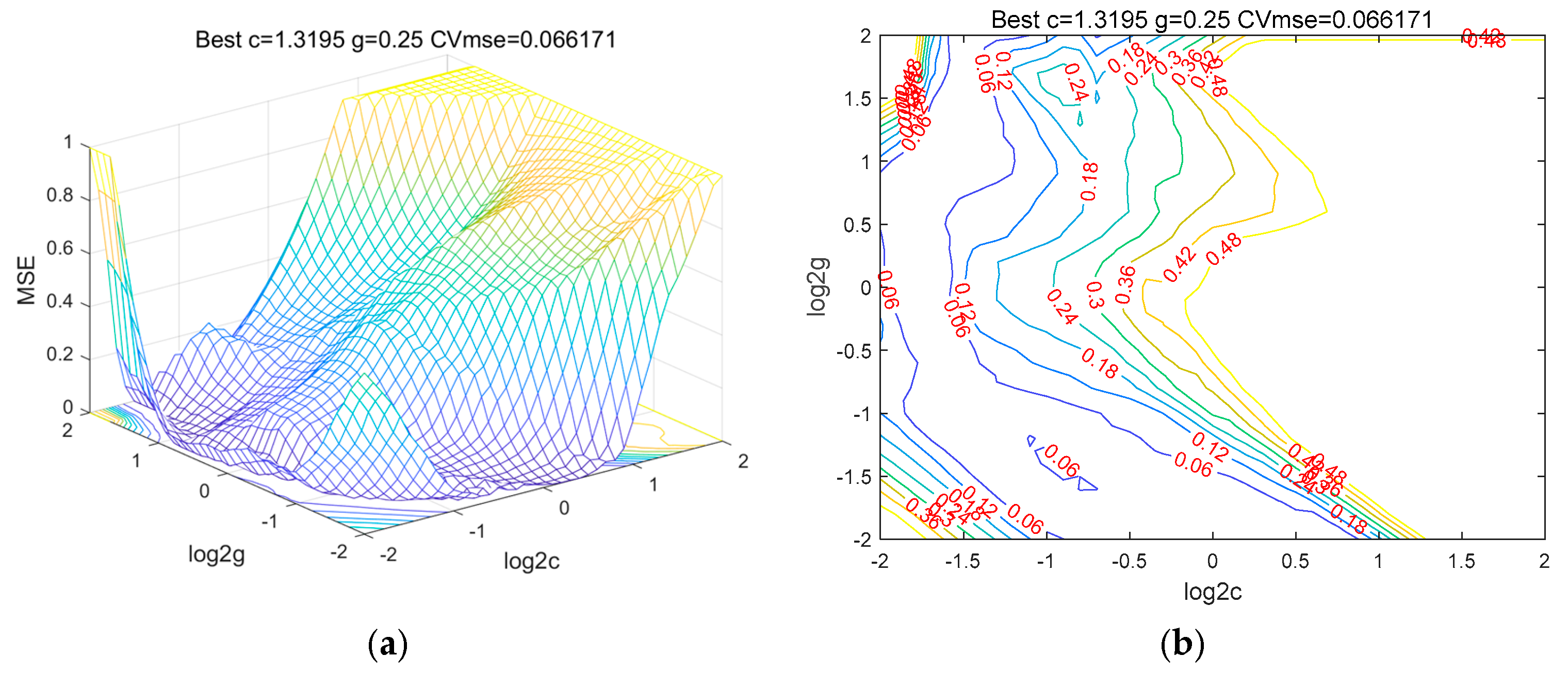
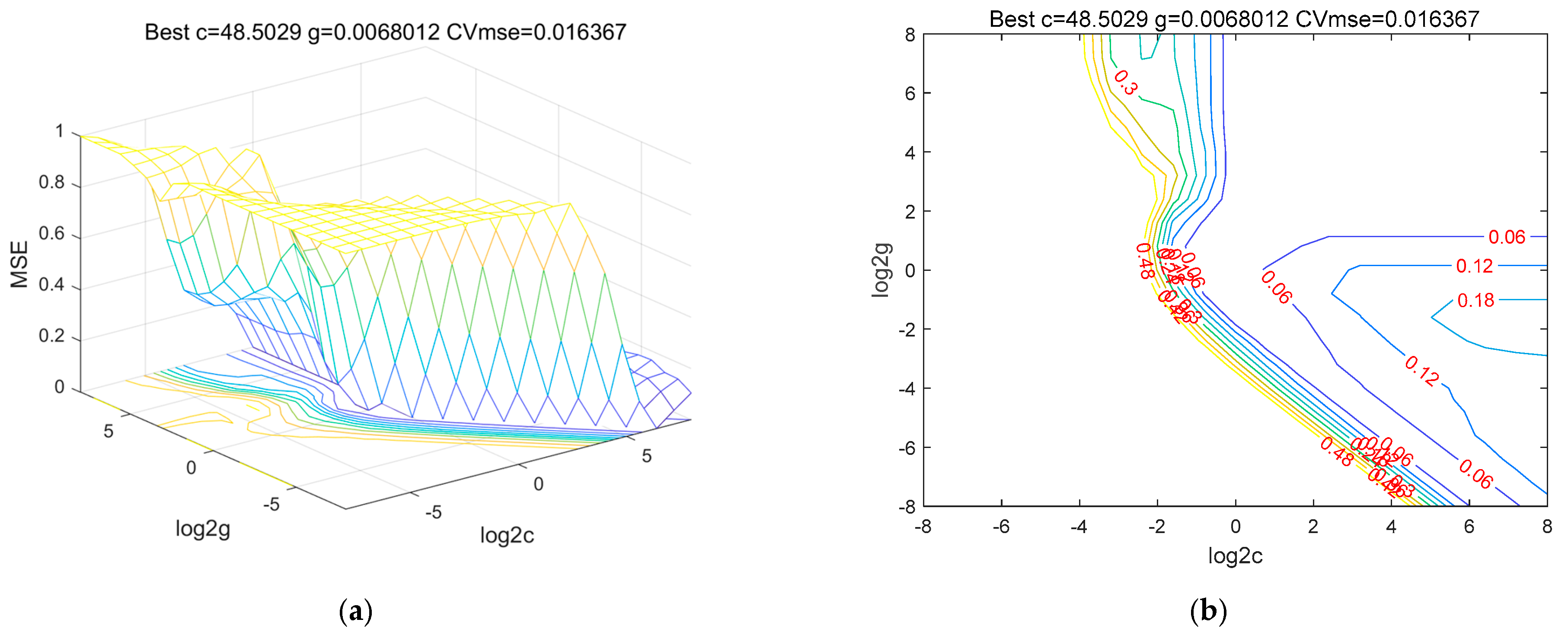
4.1. Automatic Search for Predictive Model Parameters Based on SVM

Grid search is a central strategy in the parameter tuning process of support vector machine (SVM)-based bioaerosol concentration prediction models for pinpointing the most effective penalty factor (c) and kernel function parameter (g), which involves comprehensively exploring the pre-specified hyper-parameter space and performing cross-validation (CV) for each candidate combination to assess the generalization ability of the bioaerosol concentration prediction model. By comparing the mean CV performance metrics of different combinations, the best performing parameter settings can be selected. Figure 5 shows the 3D view (a) and contour view (b) of the parameter results of the grid search obtained during the training of the SVM-based prediction model on the test data. During the grid search, a set of penalty factors (c) and kernel function parameters (g) is first set, and then the SVM-based bioaerosol concentration prediction model is trained using cross-validation for each pair of penalty factor (c) and kernel function parameter (g) combinations and its performance is evaluated. The grid search selects the best combination of parameters by calculating the validation results for all combinations.

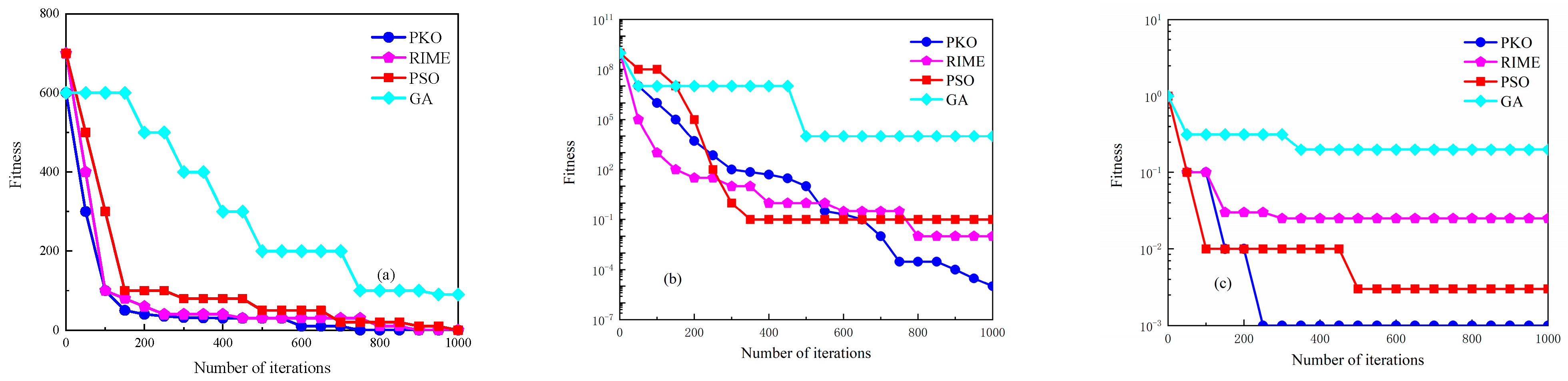
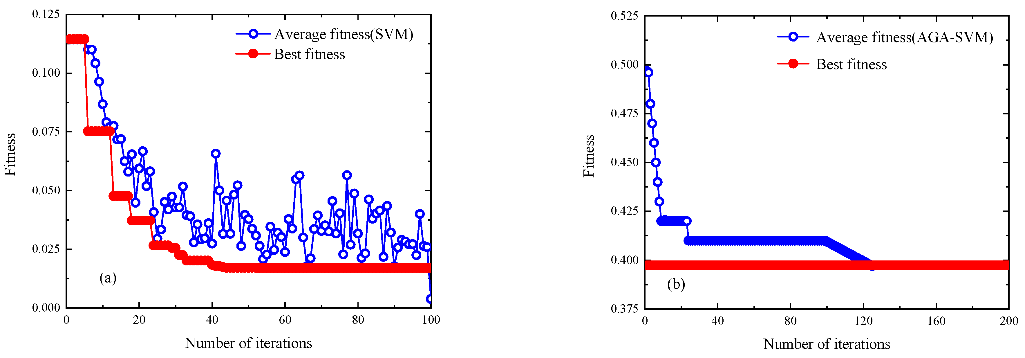
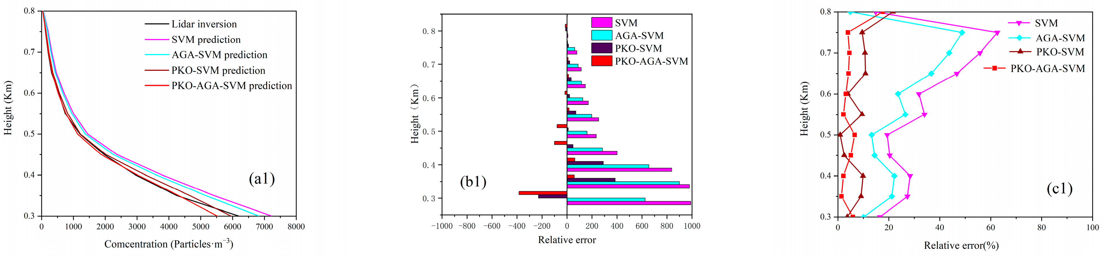
4.2. Predictive Model Optimization

In order to avoid the problem of missing the optimal solution that may be caused by grid search, in this paper, the PKO–AGA algorithm was added to optimize the bioaerosol concentration prediction model based on the SVM algorithm, which was continuously optimized by populations divided into datasets so as to form the new parameters and reach the optimal dataset solution [25,26,27]. Figure 6 shows a 3D view of the relative error (a) and a contour plot (b) of the results of the test dataset runs of the prediction model based on the PKO–AGA–SVM fusion algorithm.
Figure 7 shows the curve of the best fitness versus the mean fitness of the population obtained when the prediction model was trained to predict the test data. Figure 7a shows the population fitness curve of the prediction model based on the SVM algorithm, which shows that the population fitness curve fluctuated a lot from the graph. Figure 7b shows the population fitness curve of the prediction model-optimized SVM based on the AGA algorithm. The figure shows that the population fitness curve fluctuated a lot at the beginning, and the best fitness curve tended to be stable as the iteration proceeded. Figure 7c shows the population fitness curve of the prediction model-optimized SVM based on the PKO algorithm. The figure shows that the population fitness fluctuated more at the beginning, and as the iteration proceeded, the best fitness curve tended to be stable. The population fitness curve obtained experimentally after optimization of SVM by the PKO–AGA fusion algorithm is shown in Figure 7d. It can be seen in the figure that the PKO algorithm had the crossover selection and mutation mechanism of the AGA algorithm, which could dynamically adjust the weight of exploration and exploitation, especially when the fitness was better. The crossover and mutation operations helped to maintain the diversity of the population to avoid premature convergence, and the probability of the model falling into a locally optimal solution was reduced, although the speed of convergence may have been slower. It can be seen that the combination of the PKO algorithm and the AGA algorithm significantly improved the stability and accuracy of the model in finding the optimal solution.

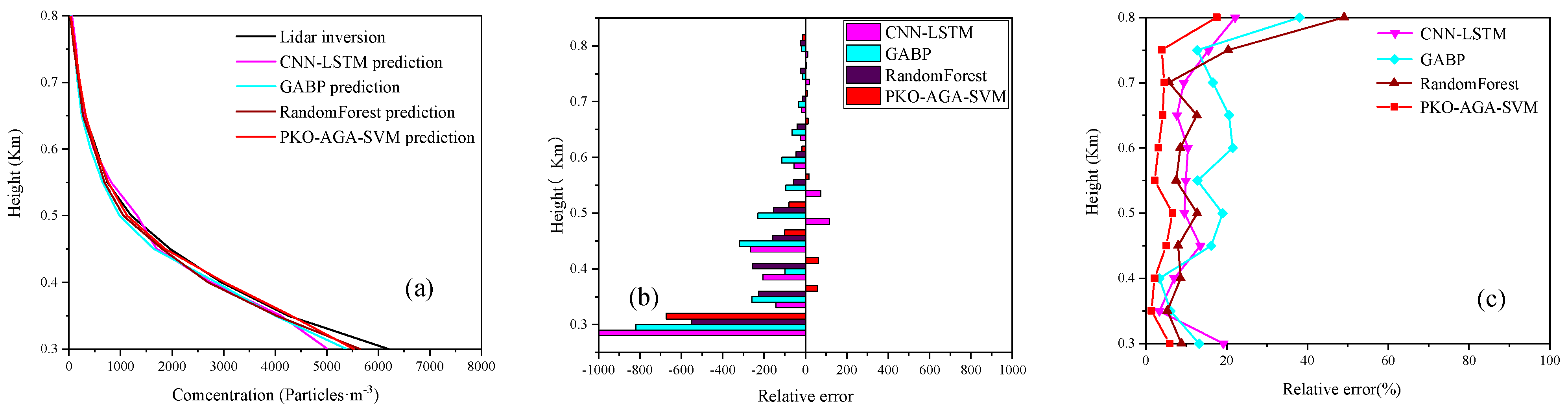
4.3. Model Prediction Accuracy Verification

In this study, a five-fold cross-validation method was used to calculate the 95% confidence intervals of the prediction errors. The data were then divided into five equal-sized subsets, and the subsets were sequentially used as the validation set. The remaining four subsets were used as the training set for relative error validation, and the results of the mean relative errors of different algorithms are shown in Table 3.
Assuming that the errors follow a normal distribution, the 95% confidence interval for the five-fold cross-validation method is calculated as:
95 % CI = E ¯ r ± 1.96 × σ r 5
where Ēr is the mean and σr is the standard deviation. The data results predicted by the different algorithm models are shown in Table 4, with PKO–AGA–SVM obtaining a mean Ēr of 12.35% and a standard deviation σr of 1.0078. The confidence interval of the PKO–AGA–SVM algorithm was calculated to be 11.106–13.594%. The PKO–AGA–SVM algorithm models were more concentrated and fluctuated less than the other algorithm models in the distribution of prediction errors on different data subsets, and the model prediction results were more stable.
In order to test the generalization effect of the predictive model with a smaller data set, this paper reduced and conducted experimental comparisons between the model training set and the test set, which were 100%, 80%, 60%, and 40% of the randomly sampled original data set, respectively. The experimental results are shown in Table 5. The experimental results show that when the amount of training data was reduced from 100% to 20%, the mean relative error of the PKO–AGA–SVM model rose from 11.57% to 14.07%, which is only 2.5%, significantly lower than that of the SVM (7.56%), AGA–SVM (3.87%), and PKO–SVM (3.08%) models. The SVM algorithm inherently has an accurate small data sample prediction ability; after optimization, the PKO–AGA–SVM fusion algorithm model alleviated the impact of data scarcity on model performance more.
In order to quantify whether the difference in performance between PKO–AGA–SVM and other models is statistically significant, this study used the Friedman test, which was used previously to complete the five-fold cross-validation, and the performance values of the models were ranked, with the results shown in Table 6.
In order to test the generalization effect of the prediction model on the dataset with unbalanced data, this study changed the composition of the model training set and test set and conducted experimental comparisons. The experimental data were 70% of the heavily polluted weather data plus 30% of the remaining weather data, and 70% of the data for mildly polluted weather and below plus 30% of the remaining weather data. The experimental results are shown in Table 7. When the amount of training data was 70% of the moderately polluted weather data and above and 30% of the remaining weather data, the average relative error of the PKO–AGA–SVM model was 13.01%, which is 1.44% higher than that of the complete dataset and lower than that of the SVM model, with an increase in prediction error of 5.71%; lower than that of the AGA–SVM model, with an increase of 5.01%; and lower than that of the PKO–SVM model, with an increase of 2.62%. When the amount of training data was 70% of the mildly polluted weather data and 30% of the remaining weather data, the average relative error of the PKO–AGA–SVM model was 12.75%, which is 1.18% higher compared to the error of the complete dataset and lower than the 3.71% increase in the prediction error of the SVM model, 2.87% higher than that of the AGA–SVM model, and 1.60% higher than that of the PKO–SVM model. The experimental results show that the PKO–AGA–SVM model was less affected by the composition of the model data, but the error still increased, mainly because after selecting the data, the training and testing dataset only accounted for about 60% of the overall data volume and the error increased to a certain extent. When the air pollution is serious, the influencing factors will become more significant, and the overall error will become larger.
In order to further validate the prediction performance of the model, CNN–LSTM, random forest, and GABP neural network prediction models were selected in this study to compare the prediction performance on the same dataset. Some of the experimental results are shown in Figure 8, and the data of the relative prediction errors are shown in Table 8.
The experimental results show that CNN–LSTM predicted fewer data when the data set was larger and more data when the data set was smaller, mainly because of the instability of the model. Random forest predicted good data when the data set was larger but higher error when the data set was smaller, mainly because of the accumulation of error due to the insufficient capture of monotonic trends by the tree model. GABP predicted better data in the case of model underfitting due to insufficient optimization. The overall error was uniform and the global search ability was poor. The PKO–AGA–SVM algorithm predicted the smallest mean relative error and was more accurate.

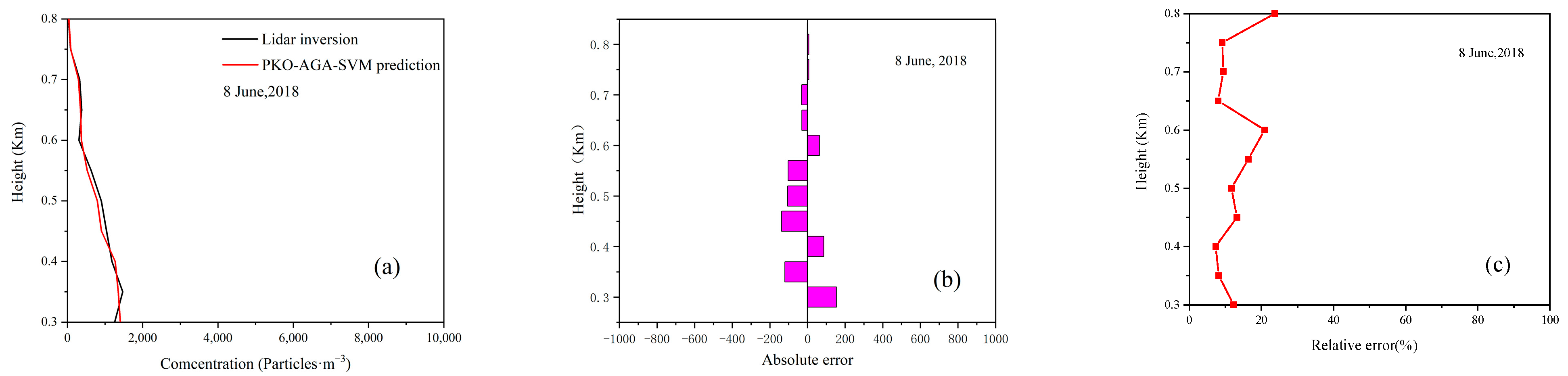
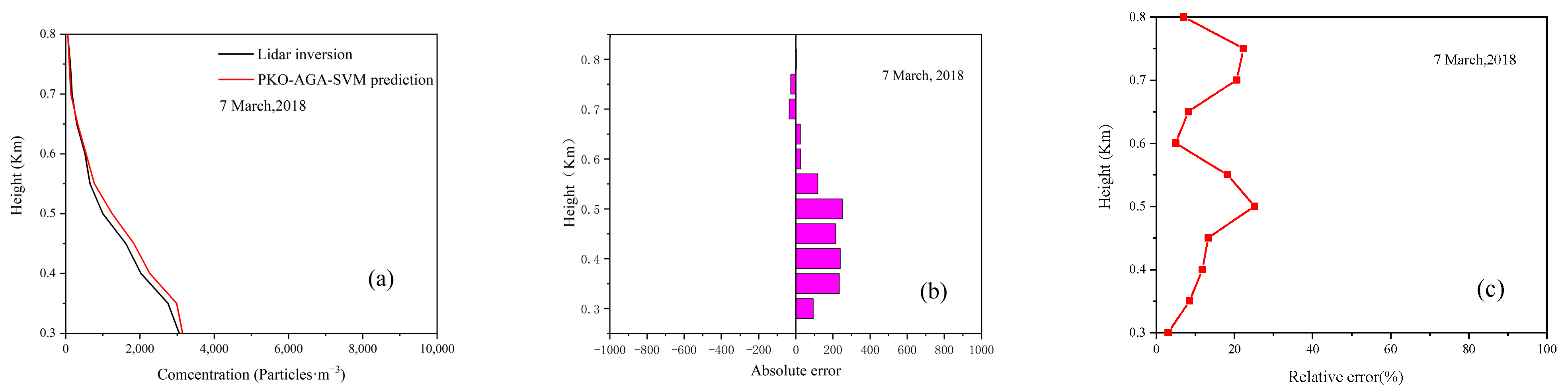
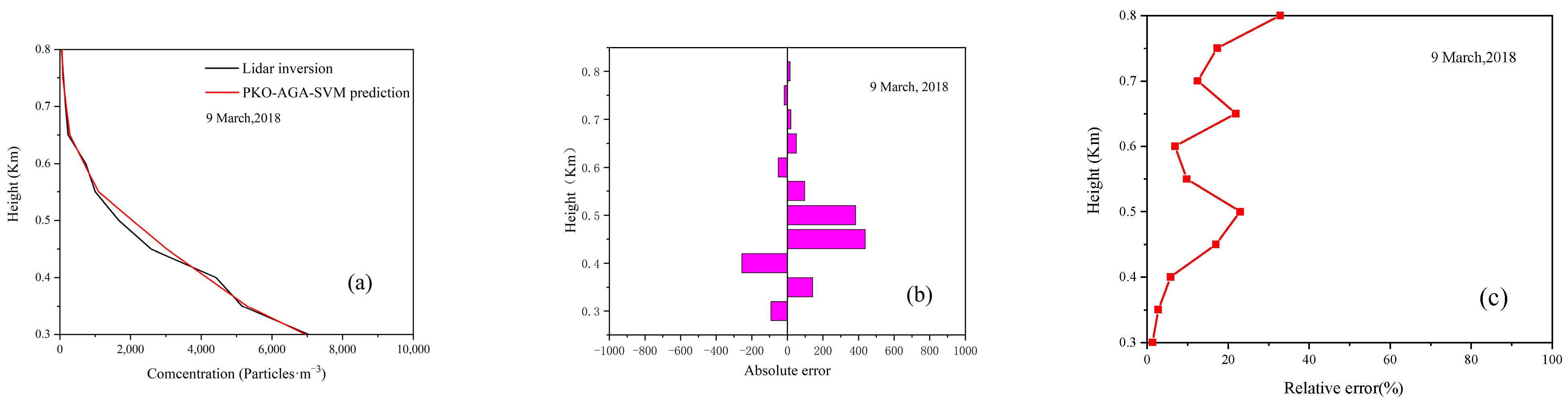
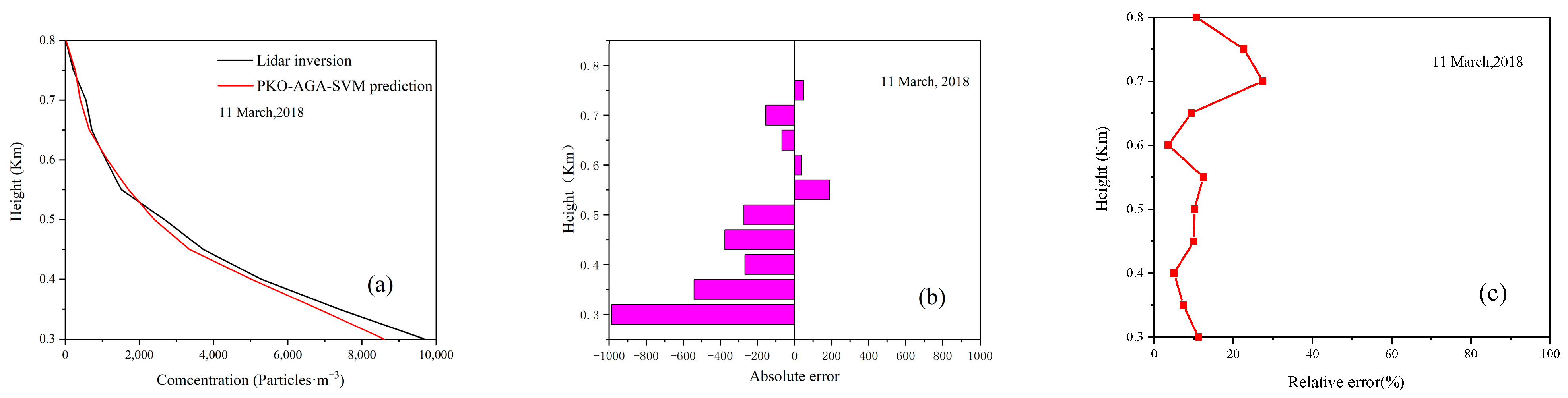
4.4. Model Prediction Experiment

After the bioaerosol concentration prediction model was trained, the prediction effect of the model was experimentally verified, and the bioaerosol concentration profiles predicted by the model were compared and analyzed with the bioaerosol concentration profiles detected by fluorescence lidar to verify the reliability of the prediction model. Figure 9a shows the bioaerosol concentration profiles detected by fluorescence lidar and those predicted by the model using different algorithms, Figure 9b shows the absolute error between the bioaerosol concentration detected by fluorescence lidar and those predicted by the model using different algorithms, Figure 9c shows the relative error between the bioaerosol concentration detected by fluorescence lidar and those predicted by the model using different algorithms, and Figure 9c shows the relative error between the bioaerosol concentration detected by fluorescence lidar and those predicted by the model using different algorithms. Among them, Figure 9a shows the results of the bioaerosol concentration profiles predicted by the SVM algorithm, the AGA–SVM algorithm, the PKO–SVM algorithm, and the PKO–AGA–SVM algorithm, and it was found that the PKO–AGA–SVM fusion algorithm demonstrated better overall fit and its prediction results were better than the real ones based on comparing the predicted values with the real values of different optimization algorithms. The overall fit and its prediction results were closer to the true values compared to other models. Figure 9b,c show that the PKO–AGA–SVM fusion algorithm can be more clearly seen in the absolute and relative error plots, which show that the PKO–AGA–SVM fusion algorithm predicted the model with less overall error. In addition, for the prediction of bioaerosol concentration profiles, the overall relative error was smaller in the lower-altitude range, but the absolute error of the model prediction was larger for larger values of actual concentration. The relative errors predicted by all algorithms showed an increasing trend with height as the height increased. The main reason for this is a combination of several factors: Firstly, the measurement accuracy of the fluorescence lidar was limited as the height increased, which affected the reliability of the data and the accuracy of the predictions. In addition, in the case of few sample data, the data were not well represented, leading to an increase in the bias of the prediction results. Table 9 shows the mean relative errors of the bioaerosol concentration profiles predicted by the model using different algorithms.
For the bioaerosol concentration prediction model using the SVM algorithm, after optimization by different algorithms, is the results were mainly reflected in the change in penalty factor c and kernel function parameter g. If the penalty factor c is too large or too small, it may cause the model generalization ability to decline. When the radial basis function (RBF) is chosen as the kernel, the kernel parameter g is a parameter that comes with the function, which implicitly determines the distribution of the data mapped into the new feature space: the larger the kernel parameter g is, the fewer support vectors there are; the smaller the kernel parameter g is, the more support vectors there are, and the number of support vectors has an effect on the training and prediction speed. The optimal value was obtained by introducing the AGA–PKO fusion algorithm to optimize the penalty factor c and kernel function parameter g of the support vector machine. The adaptive mechanism of the AGA algorithm was able to maintain the population diversity by dynamically adjusting the weight of exploration and exploitation, thus avoiding premature convergence, and it had a stronger global search capability, so it was not easy for the prediction model to fall into the local optimum. Then, the resulting optimal solution was used as a parameter for the model training and prediction. The results in Table 4 show that both the AGA and the PKO algorithms’ individually optimized predictions were better than that of the underlying SVM algorithm, while the fusion algorithm that combines AGA and PKO improved the prediction results compared to the first three algorithms, a result that confirms that the PKO–AGA–SVM fusion algorithm has better prediction performance compared to the SVM, the PKO–SVM, and the AGA–SVM algorithms.
In order to further validate the prediction ability of the PKO–AGA–SVM fusion algorithm model, the PKO–AGA–SVM fusion algorithm model was utilized in the paper to predict the bioaerosol concentration profiles under different atmospheric conditions. Five different air quality levels were selected for prediction analysis, which were excellent, good, mildly polluted, moderately polluted, and heavily polluted weather. The prediction performance of the PKO–AGA–SVM algorithm was further evaluated by predicting the bioaerosol concentration and comparing the prediction results with the fluorescence lidar inversion data. The prediction results are shown in Figure 10 (excellent weather), Figure 11 (good weather), Figure 12 (mildly polluted weather), Figure 13 (moderately polluted weather), and Figure 14 (heavily polluted weather). Figure 10a shows that the bioaerosol concentration predicted by the model at 0.35 km was 1350 particles·m−3, Figure 10b shows an absolute error of 120 particles·m−3, and Figure 10c shows a relative error of 8.16%. Figure 11a shows that the bioaerosol concentration predicted by the model at 0.35 km was 2990 particles·m−3, Figure 11b shows an absolute error of 234.5 particles·m−3, and Figure 11c shows a relative error of 8.51%. Figure 12a shows that the bioaerosol concentration predicted by the model at 0.35 km was 3510 particles·m−3, Figure 12b shows an absolute error of 371 particles·m−3, and Figure 12c shows a relative error of 9.56%. Figure 13a shows that the bioaerosol concentration predicted by the model at 0.35 km was 5299 particles·m−3, Figure 13b shows an absolute error of 142.2 particles·m−3, and Figure 13c shows a relative error of 2.76%. Figure 14a shows that the bioaerosol concentration predicted by the model at 0.35 km was 6840 particles·m−3, Figure 14b shows an absolute error of 542 particles·m−3, and Figure 14c shows a relative error of 7.34%. The experimental results show that with the increase in the degree of pollution in the atmospheric environment, the bioaerosol concentration predicted by the PKO–AGA–SVM fusion algorithm model also showed a corresponding increasing trend, the absolute error increased but the relative error stayed within 12%, and there was no increasing or decreasing trend, which indicates that there was no obvious gap between the prediction effect of the model in the case of different weather.
Table 10 shows the prediction under different levels of atmospheric pollution. The overall error is about 12%, and with better weather conditions, the relative error increased slightly. The reason is mainly because of the lower concentration of bioaerosols. The sample data were fewer, so the mean error was susceptible to individual extreme values of the interference data, so the error was slightly elevated. Worse weather conditions with higher bioaerosol concentrations and more sample data increased the absolute error, and the mean relative error was almost the same. The experimental results show that the PKO–AGA–SVM fusion algorithm maintained good prediction performance under all types of weather conditions, which verifies the effectiveness and reliability of the algorithm in dealing with the prediction of bioaerosol concentration under complex environmental conditions. Table 10 shows the mean relative errors in the prediction of bioaerosol concentration for different atmospheric pollution scenarios by the model using the PKO–AGA–SVM fusion algorithm. These results indicate that the prediction model showed high accuracy and stability under different atmospheric environmental conditions, which can provide a new research approach and technical support for an early warning system of atmospheric bioaerosol concentration.
In order to further investigate the influence of pollutants on bioaerosol concentration in different pollution environments, this study analyzed the predicted influences on the input parameters of the model and plotted SHAP diagrams, as shown in Figure 15. The experimental results show that bioaerosol concentration was strongly influenced by temperature and humidity, wind speed, and pollutants such as PM2.5, and gases to a lesser extent.

5. Conclusions

In this paper, a machine learning prediction model based on the PKO–AGA–SVM fusion algorithm is proposed for predicting bioaerosol concentrations in the atmosphere. The model combines atmospheric environmental parameters (e.g., PM2.5, PM10, SO2, NO2, CO, O3, temperature, humidity, etc.) as well as bioaerosol concentration data detected by fluorescence lidar. Considering that the bioaerosol concentration is significantly affected by atmospheric environmental factors, the study in this paper used the relevant environmental parameter dataset as the input variable and the fluorescence lidar-detected bioaerosol concentration dataset as the output variable for model training. The prediction model optimizes the penalty coefficient c and kernel function parameter g of the support vector machine (SVM) model to avoid the problem of local optimal solution that may occur in the traditional grid search method, and a combination of the pied kingfisher algorithm (PKO) and the adaptive genetic algorithm (AGA) is used. The model prediction experiments show that the mean prediction error of the PKO–AGA–SVM prediction model was 11.572%, which is significantly lower than the prediction errors of the PKO–SVM (16.934%), AGA–SVM (20.754%), and conventional SVM (25.794%) models. The prediction model of the PKO–AGA–SVM fusion algorithm was utilized to predict bioaerosol concentration under different atmospheric pollution scenarios, and the mean prediction error was 12.749% when the air quality was excellent, 13.001% when the air quality was good, 10.513% when the air quality was mildly polluted, 13.715% when the air quality was moderately polluted, and 11.823% when the air quality was heavily polluted. When the air quality was moderate, the mean error of prediction was 13.715%, and when the air quality was heavily polluted, the mean error of prediction was 11.823%. The experimental results show that the optimization algorithm using the PKO and AGA algorithms combined with SVM had better population fitness compared with the AGA algorithm alone or the PKO algorithm alone combined with SVM, which effectively improved the prediction accuracy of the PKO–AGA–SVM fusion algorithm model. The model prediction results show that the model performed well under different atmospheric pollution scenarios, which provides reliable proof for the prediction of atmospheric bioaerosol concentration.

Author Contributions

Methodology, Z.R.; Software, Z.R.; Validation, Z.R.; Formal analysis, Z.R., J.M. and X.G.; Investigation, Z.R.; Resources, Z.R.; Data curation, Z.R., Y.L. and H.Z. All authors have read and agreed to the published version of the manuscript.

Funding

This work was supported by the National Natural Science Foundation of China (grant Nos. 42465007, 42105140).

Institutional Review Board Statement

Not applicable.

Informed Consent Statement

Not applicable.

Data Availability Statement

The original contributions presented in this study are included in the article. Further inquiries can be directed to the corresponding author.

Acknowledgments

The data and data analysis method are available upon request.

Conflicts of Interest

The authors declare no conflict of interest.

References

  1. Kim, K.S.; Lee, I.; Lee, J. Synergetic Chemo-Machaon Antimicrobial Puncturable Nanostructures for Efficient Bioaerosol Removal. Biochip J. 2024, 18, 439–452. [Google Scholar] [CrossRef]
  2. da Silva, J.C.R.; Lopes, M.C.d.S.; Prates, K.V.M.C.; Mantoani, M.C.; Martins, L.D. Characterization of indoor airborne particulate matter and bioaerosols in wood-fired pizzeria kitchens. Discov. Environ. 2024, 2, 107. [Google Scholar] [CrossRef]
  3. Nasser, N.I.; Al-Hadrawi, M.K.; Oleiwi, S.A.; Mohsin, A.A. The Diversity in Dust Fungal Spores Concentration at Four Districts of Al-Najaf Environment and their Potential Correlation with Asthma. J. Pure Appl. Microbiol. 2019, 13, 273–280. [Google Scholar] [CrossRef]
  4. Liu, H.; Zhang, X.; Zhang, H.; Yao, X.; Zhou, M.; Wang, J.; He, Z.; Zhang, H.; Lou, L.; Mao, W.; et al. Effect of air pollution on the total bacteria and pathogenic bacteria in different sizes of particulate matter. Environ. Pollut. 2018, 233, 483–493. [Google Scholar] [CrossRef]
  5. Liggio, J.; Li, S.M. Organo sulfate formation during the uptake of pinon aldehyde on acidic sulfate aerosols. Geophys. Res. Lett. 2006, 33, 338–345. [Google Scholar] [CrossRef]
  6. Li, X.; Cheng, X.; Wu, W.; Wang, Q.; Tong, Z.; Zhang, X.; Deng, D.; Li, Y.; Gao, X. An improved wavelet de-noising-based back propagation neural network model to forecast the bioaerosol concentration. Aerosol Sci. Technol. 2020, 55, 352–360. [Google Scholar] [CrossRef]
  7. Goudarzi, G.; Birgani, Y.T.; Assarehzadegan, M.-A.; Neisi, A.; Dastoorpoor, M.; Sorooshian, A.; Yazdani, M. Prediction of airborne pollen concentrations by artificial neural network and their relationship with meteorological parameters and air pollutants. J. Environ. Health Sci. Eng. 2022, 20, 251–264. [Google Scholar] [CrossRef]
  8. Rao, Z.; He, T.; Hua, D.; Wang, Y.; Wang, X.; Chen, Y.; Le, J. Preliminary measurements of fluorescent aerosol number concentrations using a laser-induced fluorescence lidar. Appl. Opt. 2018, 57, 7211–7215. [Google Scholar] [CrossRef]
  9. Bai, Y.; Ren, P.; Feng, P.; Yan, H.; Li, W. Shift in rhizosphere and endophytic bacterial communities of tomato caused by salinity and grafting. Sci. Total Environ. 2020, 734, 139388. [Google Scholar] [CrossRef]
  10. Chen, Q.; Mu, Z.; Xu, L.; Wang, M.; Wang, J.; Shan, M.; Fan, X.; Song, J.; Wang, Y.; Lin, P.; et al. Triplet-State Organic Matter in Atmospheric Aerosols: Formation Characteristics and Potential Effects on Aerosol Aging. Atmos. Environ. 2021, 252, 118343. [Google Scholar] [CrossRef]
  11. Shoshana, O.; Baratz, A. Daytime measurements of Bioaerosol Simulants using a Hyperspectral Laser-Induced Fluorescence LIDAR for Biosphere Research. J. Environ. Chem. Eng. 2020, 8, 104392. [Google Scholar] [CrossRef]
  12. Yang, J.; Zheng, H.; Ma, Y.; Zhao, P.; Zhou, H.; Li, S.; Wang, X.H. Background noise model of spaceborne photon-counting lidars over oceans and aerosol optical depth retrieval from ICESat-2 noise data. Remote Sens. Environ. 2023, 299, 113858. [Google Scholar] [CrossRef]
  13. Lin, B.L.; Tokai, A.; Nakanishi, J. Approaches for Establishing Predicted-No-Effect Concentrations for Population-Level Ecological Risk Assessment in the Context of Chemical Substances Management. Environ. Sci. Technol. 2005, 39, 4833. [Google Scholar] [CrossRef] [PubMed]
  14. Matsuo, T.; Takimoto, M.; Tanaka, S.; Futamura, A.; Shimadera, H.; Kondo, A. Developing an Automatic Asbestos Detection Method Based on a Convolutional Neural Network and Support Vector Machine. Appl. Sci. 2024, 14, 9408. [Google Scholar] [CrossRef]
  15. Pratt, G.C.; Wu, C.Y.; Bock, D.; Adgate, J.L.; Ramachandran, G.; Stock, T.H.; Morandi, M.; Sexton, K. Comparing air dispersion model predictions with measured concentrations of VOCs in urban communities. Environ. Sci. Technol. 2004, 38, 1949–1959. [Google Scholar] [CrossRef]
  16. Karadurmus, E.; Berber, R. Dynamic Simulation and Parameter Estimation in River Streams. Environ. Technol. 2004, 25, 471–479. [Google Scholar] [CrossRef]
  17. Halteh, K.; AlKhoury, R.; Ziadat, S.A.; Gepp, A.; Kumar, K. Using machine learning techniques to assess the financial impact of the COVID-19 pandemic on the global aviation industry. Transp. Res. Interdiscip. Perspect. 2024, 24, 101043. [Google Scholar] [CrossRef]
  18. Salawu, S.; He, Y.; Lumsden, J. Approaches to automated detection of cyberbullying: A survey. IEEE Trans. Affect. Comput. 2017, 11, 3–24. [Google Scholar] [CrossRef]
  19. Lee, J.; Kang, S. GA based meta-modeling of BPN architecture for constrained approximate optimization. Int. J. Solids Struct. 2007, 44, 5980–5993. [Google Scholar] [CrossRef]
  20. Akin, P. A new hybrid approach based on genetic algorithm and support vector machine methods for hyperparameter optimization in synthetic minority over-sampling technique (SMOTE). Aims Math. 2023, 8, 9400–9415. [Google Scholar] [CrossRef]
  21. Srinivas, M.; Patnaik, L.M. Adaptive probabilities of crossover and mutation in genetic algorithms. IEEE Trans. Syst. Man Cybern. 2002, 24, 656–667. [Google Scholar] [CrossRef]
  22. Mak, K.L.; Wong, Y.S.; Wang, X.X. An Adaptive Genetic Algorithm for Manufacturing Cell Formation. Int. J. Adv. Manuf. Technol. 2000, 16, 491–497. [Google Scholar] [CrossRef]
  23. Duan, K.; Fong, S.; Siu, S.W.I.; Song, W.; Guan, S.S.-U. Adaptive Incremental Genetic Algorithm for Task Scheduling in Cloud Environments. Symmetry 2018, 10, 168. [Google Scholar] [CrossRef]
  24. Park, S.S.; Kim, J.H. Possible sources of two size-resolved water-soluble organic carbon fractions at a roadway site during fall season. Atmos. Environ. 2014, 94, 134–143. [Google Scholar] [CrossRef]
  25. Guo, H.; Ling, Z.; Cheung, K.; Wang, D.; Simpson, I.; Blake, D. Acetone in the atmosphere of Hong Kong: Abundance, sources and photochemical precursors. Atmos. Environ. 2013, 65, 80–88. [Google Scholar] [CrossRef]
  26. Giuliani, C.; Biggs, D.; Nguyen, T.T.; Marasco, E.; De Fanti, S.; Garagnani, P.; Le Phan, M.T.; Nguyen, V.N.; Luiselli, D.; Romeo, G. First evidence of association between past environmental exposure to dioxin and DNA methylation of CYP1A1 and IGF2 genes in present day Vietnamese population. Environ. Pollut. 2018, 242, 976–985. [Google Scholar] [CrossRef]
  27. Srivastava, A.N. Data Mining: Concepts, Models, Methods, and Algorithms. ASME J. Comput. Inf. Sci. Eng. 2005, 5, 394–395. [Google Scholar] [CrossRef]
Figure 1. Working principle diagram of atmospheric bioaerosol fluorescence lidar system.
Atmosphere 16 00638 g001
Figure 2. CEC2005 standardized test functions: F11 test result (a), F13 test result (b), F15 test result (c).
Atmosphere 16 00638 g002
Figure 3. Flowchart of PKO–AGA–SVM fusion algorithm to optimize the prediction model.
Atmosphere 16 00638 g003
Figure 4. Flow chart of bioaerosol concentration prediction model based on the PKO–AGA–SVM fusion algorithm.
Atmosphere 16 00638 g004
Figure 5. 3D view of relative error (a) and contour plot (b) of the results of the test dataset runs of the prediction model based on SVM.
Atmosphere 16 00638 g005
Figure 6. 3D view of relative error (a) and contour plot (b) of the results of the test dataset runs of the prediction model based on the PKO–AGA–SVM fusion algorithm.
Atmosphere 16 00638 g006
Figure 7. Curves of best fitness versus mean fitness of the population obtained when predicting the test data during training of the prediction model: (a) SVM, (b) AGA–SVM, (c) PKO–SVM, and (d) PKO–AGA–SVM.
Atmosphere 16 00638 g007aAtmosphere 16 00638 g007b
Figure 8. Results of different model predictions: (a) bioaerosol concentration contours, (b) absolute error, (c) relative error.
Atmosphere 16 00638 g008
Figure 9. PKO–AGA–SVM model prediction results: (a) bioaerosol concentration contours, (b) absolute error, (c) relative error.
Atmosphere 16 00638 g009aAtmosphere 16 00638 g009b
Figure 10. Plot of the PKO–AGA–SVM model predicting superior weather results (a), absolute error (b), relative error (c).
Atmosphere 16 00638 g010
Figure 11. Plot of the PKO–AGA–SVM model predicting good weather results (a), absolute error (b), relative error (c).
Atmosphere 16 00638 g011
Figure 12. Plot of the PKO–AGA–SVM model results for predicting mildly polluted weather (a), absolute error (b), relative error (c).
Atmosphere 16 00638 g012
Figure 13. Plot of the PKO–AGA–SVM model results for predicting moderately polluted weather (a), absolute error (b), relative error (c).
Atmosphere 16 00638 g013
Figure 14. Plot of the PKO–AGA–SVM model results for predicting heavily polluted weather (a), absolute error (b), relative error (c).
Atmosphere 16 00638 g014
Figure 15. SHAP plot of model-predicted impact factors.
Atmosphere 16 00638 g015
Table 1. Main parameters of the fluorescence lidar.
DefinitionReference Value
Pulse energy60 mJ
Field of view of the telescope0.5 mrad
Quantum efficiency of the PMT0.2
Transmission of the receiving optical train0.3
Filter bandwidth10 nm
Diameter of the telescope25 cm
Laser wavelength266 nm
Fluorescence wavelength300~460 nm
Pulse repetition frequency10 Hz
Detector frequency bandwidth5 Mz
Effective cross-sectional area for the fluorescence inelastic scattering10−12 cm2 sr−1 nm−1
Reception efficiency of the entire optical system for the fluorescence wavelength0.3
Table 2. Specific input and output information of the bioaerosol concentration prediction model based on the PKO–AGA–SVM fusion algorithm.
Input/OutputInput Parameter NumberVariant
1PM2.5
2PM10
3CO
4NO2
Input5O3
6SO2
7Temperature
8Humidity
9Wind speed
Output1~11Bioaerosol concentrations at different hights
Table 3. Mean relative error of different algorithms.
Serial NumberMean Relative Error (%)
SVMAGA–SVMPKO–SVMPKO–AGA–SVM
125.7920.7516.9311.57
227.4522.1018.2012.8
326.921.317.512.1
429.824.519.613.4
524.319.815.710.9
Table 4. Analysis of results predicted by different algorithmic models.
AlgorithmStandard DeviationMean Values (%)Confidence Interval (%)
SVM2.0426.84824.31–29.39
AGA–SVM1.5921.6919.48–23.90
PKO–SVM1.31717.78616.716–18.856
PKO–AGA–SVM1.007812.3511.106–13.594
Table 5. Model prediction error for different training data shares.
Percentage of DataSVM (%)AGA–SVM (%)PKO–SVM (%)PKO–AGA–SVM (%)
10025.7920.7516.9311.57
8028.1522.1817.8212.44
6031.0223.9519.1713.61
4033.3524.6220.0114.07
Table 6. Cross-validation performance.
TimesSVMAGA–SVMPKO–SVMPKO–AGA–SVM
14321
24321
34321
44321
54321
Table 7. Unbalanced training data to predict relative error.
Percentage of DataSVM (%)AGA–SVM (%)PKO–SVM (%)PKO–AGA–SVM (%)
Heavily polluted weather data 70%, remaining 30%31.525.7619.5513.01
Lightly polluted weather data 70%, remaining 30%29.623.6218.5312.75
Table 8. Mean relative error of the different models.
Optimization AlgorithmMean Relative Error (%)
PKO–AGA–SVM9.13
CNN–LSTM12.4
Random forest14.6
GABP13.8
Table 9. Mean relative error of model predictions using different algorithms.
Optimization AlgorithmMean Relative Error (%)
SVM25.79
AGA–SVM20.75
PKO–SVM16.93
PKO–AGA–SVM11.57
Table 10. Mean relative errors of the PKO–AGA–SVM fusion algorithm model for predicting bioaerosol concentrations at different atmospheric pollution levels.
Weather ConditionsMean Relative Error (%)
Excellent12.75
Good13.01
Mildly polluted10.51
Moderately pollution11.72
Heavily polluted11.83
Disclaimer/Publisher’s Note: The statements, opinions and data contained in all publications are solely those of the individual author(s) and contributor(s) and not of MDPI and/or the editor(s). MDPI and/or the editor(s) disclaim responsibility for any injury to people or property resulting from any ideas, methods, instructions or products referred to in the content.

