Improvements in Turbulent Jet Particle Dispersion Modeling and Its Validation with DNS

Abstract

Particle dispersion models (PDMs) are essential to capture the influence of unresolved turbulent eddies on particle transport in computational fluid dynamics (CFD) simulations. However, the validation of these models remains challenging, especially when relying on experimental data or CFD simulations that are based on turbulence models. In this work, we use time-averaged data obtained in a direct numerical simulation (DNS) instead of relying on turbulence models to model particle dispersion. In addition, a new particle dispersion model is presented, referred to as the limited particle–eddy interaction time (LPI) model. For a detailed and systematic evaluation of the new LPI model, we compare its performance with that of other commonly used models, such as the mean particle–eddy interaction time (MPI) model implemented in OpenFOAM^® and the randomized particle–eddy interaction time (RPI) model from the literature. The MPI model shows good agreement with the DNS for the largest particles tested (Stokes number, St = 0.2) but exhibits erratic and unphysical trajectories for smaller particles (St ≤ 0.05). To mitigate this erratic behavior, we have adjusted the eddy interaction time in the new LPI model.

1. Introduction

The interaction between turbulent eddies and aerosol particles plays a key role in particle dispersion. Without turbulence, particles would follow similar trajectories with minimal separation, resulting in limited dispersion. This process is important in several contexts, such as wind-driven pollination [1] and the dispersion of exhaled aerosol particles [2]. When it comes to respiratory events such as coughing, the effect of turbulent dispersion also significantly affects the evaporation time and the mean velocity of the particle cloud [3].

A common way to predict the flow fields in the applications discussed above is to solve the steady or unsteady Reynolds-averaged Navier–Stokes (RANS and URANS) equations to obtain the mean flow fields at a low computational cost. However, these methods do not capture all turbulent scales as they use turbulence models to account for these small scales. As a result, when particle motion is of interest, particle dispersion models (PDMs) are used to account for the effects of the unresolved velocity fluctuations induced by the unresolved small-scale turbulent eddies and the duration of the particle–eddy interactions, which are typically based on the turbulent kinetic energy (k) and its dissipation rate ($ϵ$).

In standard particle dispersion models, the eddy interaction time is predicted as a function of the so-called eddy lifetime (ELT) and the time that it takes a particle to pass through an eddy [4]. Such a stochastic dispersion model is implemented in the open-source computational fluid dynamics (CFD) toolkit OpenFOAM^® [5], which Zhang et al. [6] used to investigate particles with Stokes numbers below unity (0.3), around unity (1.4), and above unity (11.2). By modifying the time that a particle requires to pass through an eddy, they enhanced the predictive accuracy of RANS simulations combined with their newly developed PDM, achieving better agreement with the DNS results.

With respect to the ELT, it is generally assumed that a particle remains within an eddy for the duration of the ELT, for which the perturbation velocity of the particle’s carrier flow (both magnitude and direction) remains constant. As a result, the particle trajectory is a straight line, ignoring the rotational motion of the modeled eddy. The overall effect of this simplification is the possible overprediction of the particle dispersion [2].

To improve the prediction of particle dispersion, we propose stopping the particle interaction with the eddy once the distance traveled by the particle within the eddy exceeds a certain threshold with respect to the characteristic eddy length. This approach limits the possible displacement caused by a single eddy, thereby reducing the potential overestimation of the particle dispersion.

In addition, PDMs are often validated by comparison with experimental data [4]. The main disadvantage is that the dispersion models do not only depend on the mean velocity $\langle \mathit{U}\rangle$ but also on k and $ϵ$, which are usually not provided. On the other hand, the k and $ϵ$ predicted in RANS/URANS simulations cannot be regarded as ground truth since they are the results of the statistical turbulence models used, which are known to have limited reliability. Therefore, validating the results of a dispersion model that depends on the k and $ϵ$ modeled in RANS and URANS simulations is not appropriate. In addition, experiments that simultaneously provide three-dimensional Eulerian flow fields and particle trajectories are rare and difficult to perform, especially when dealing with small particles that require intense illumination to be captured by cameras.

Therefore, in the present work, validation is performed by means of a direct numerical simulation (DNS), which resolves all turbulence scales and provides comprehensive flow data. However, to mimic a URANS simulation, the fully resolved DNS velocity field is time-averaged to filter out the fine-scale turbulent structures and to calculate the k and $ϵ$ required in the dispersion model. The resulting particle dispersion can then be directly compared to that of the full DNS. Since the boundary conditions and mean flow field are the same, any differences in particle dispersion must be caused by the dispersion model itself, ensuring its proper and independent validation.

The implementation of this approach requires the definition of time windows over which the DNS flow field is to be averaged. Calculating a conventional arithmetic mean over N time steps would require storing all the data from these N steps, which is not feasible due to the large memory requirements of DNS. To solve this problem, we use exponential smoothing [7,8], which is based on only the current time-step data and the running mean. This efficient method has previously been used to average large eddy simulation flow fields [9], and it allows for real-time time averaging in the course of the DNS.

In summary, the described approach is performed in the following three steps:

• Mimicking the statistical velocity fluctuations of URANS simulations via the exponential smoothing of DNS fields using real-time time averaging;
• Modifying an existing particle dispersion model by limiting the particle displacement within an eddy with respect to its size;
• Validating the particle trajectories predicted with the new model by comparing them with those of a DNS.

2. Methodology

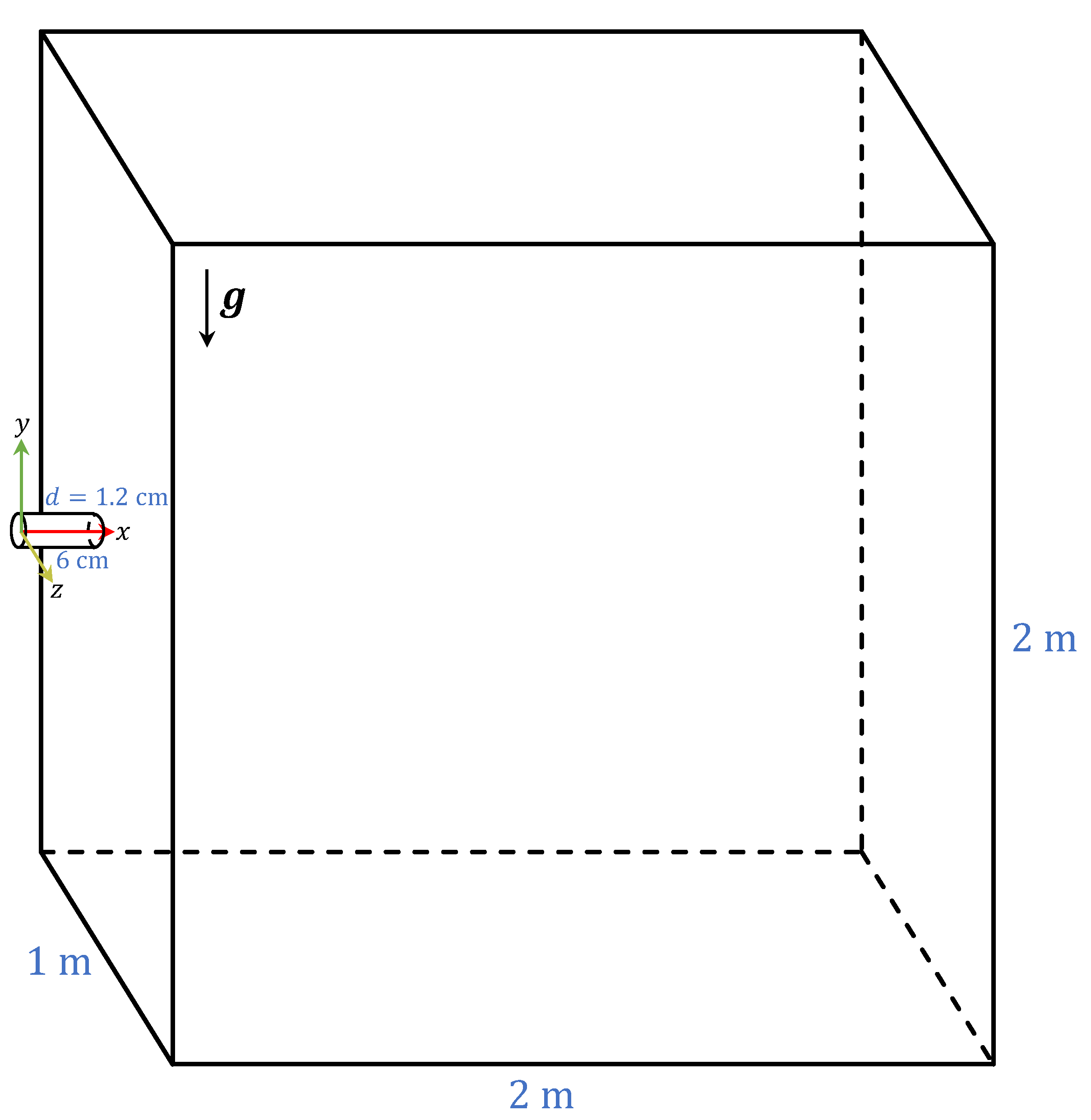
2.1. Simulation Setup and DNS Fields

A simplified but representative scenario of human exhalation was simulated in a confined space of $2\mathrm{m}\times 2\mathrm{m}\times 1\mathrm{m}$. A circular pipe was attached to the room wall at a height of 1 m, representing the mouth opening, which was 6 cm long and had a diameter of $d=1.2$ cm. The computational domain is shown in Figure 1.

The flow is governed by the incompressible Navier–Stokes equations. However, the differences in the temperature and vapor concentration between the ambient air and the exhaled breath lead to density variations and a non-negligible buoyancy effect. The exhaled air is defined at the inlet at a constant temperature of 34 °C and 90% relative humidity (RH), while the ambient air is introduced at a temperature of 20 °C with 50% RH. To account for these effects on the velocity field, the temperature T and the vapor concentration C fields are coupled to the velocity field using the Boussinesq approximation [10]:

$${\displaystyle \frac{\partial \mathit{U}}{\partial t}}+(\mathit{U}·\nabla )\mathit{U}=-{\displaystyle \frac{1}{\rho }}\nabla p+v{\nabla }^2\mathit{U}-\mathit{g}\left(\beta \left(T-T_{\mathrm{a}}\right)+\gamma \left(C-C_{\mathrm{a}}\right)\right),$$

(1)

$${\displaystyle \frac{\partial T}{\partial t}}=\nabla ·(\kappa \nabla T)-\nabla ·\left(\mathit{U}T\right),$$

(2)

$${\displaystyle \frac{\partial C}{\partial t}}=\nabla ·(D\nabla C)-\nabla ·\left(\mathit{U}C\right).$$

(3)

Equations (1)–(3) are discretized using fourth-order accurate central differences to predict the flow variables at the cell centers of a Cartesian grid consisting of hexahedral cells. The discretized equations are solved using a finite volume method provided by OpenFOAM^®v2406 (ESI Group, 10 avenue Aristide Briand, 92220 Bagneux, France) [5]. To perform a DNS, we implement the projection method [11] for velocity–pressure coupling and an explicit second-order accurate Euler-leapfrog time-stepping scheme. Kath and Wagner [12] showed that the employed method is sufficiently accurate to perform a DNS by comparing the results of a turbulent channel flow obtained in a DNS using a Cartesian grid and the above-discussed method with those from other DNS approaches, including a spectral method. The time-step size for the DNS is set in accordance with the von Neumann stability criterion derived in [13], which is satisfied with an explicit time step of $\Delta t={10}^{-4}$ s.

The maximum cell width of 3.5 mm is used, and the cells are linearly refined near the pipe region, as shown in Figure 2, where the grid is isotropic with a width of 0.8 mm inside the pipe. In the x-direction, the grid width of the room increases linearly from 0.8 mm at $x=0.06$ m and reaches 3.5 mm at $x=1$ m. In the y- and z-directions, the grid width remains constant when the absolute y and z distances are smaller than the pipe radius and then increases linearly from 0.8 mm to 3.5 mm at y and z equal to 0.5 m. Compared to our previous study [2], where a DNS of a cough puff was performed, the mesh used in the refinement region is even finer. Using the relation $\eta \sim dR{e}^{-3/4}$, where $\eta$ is the Kolmogorov length scale and $R{e}_{jet}={\mathit{U}}_{jet}d/\nu$ is the jet Reynolds number, with ${\mathit{U}}_{jet}$ being the bulk expiratory velocity magnitude of a jet (assumed to be the peak velocity in the case of a cough), the Kolmogorov scale of a breath can be estimated. Based on this scaling—with the information that the bulk velocity of a breath is 16% of that of a cough, and the mouth diameter d is about half the mouth diameter during a cough—the Kolmogorov length scale is at least three times larger for a breath than for a cough. This indicates that the current mesh resolves the smallest turbulent length scales present in a breath jet.

We define a steady homogeneous velocity profile at the inlet of the pipe as a Dirichlet boundary condition. Since human exhalation is periodic, it is not possible to simultaneously reproduce the volumetric flow rate and the momentum of real human exhalation with a steady pipe flow. We therefore opt to mimic the average momentum of female human exhalation [14] by doubling the typical average volumetric flow rate, resulting in a pipe flow rate of 12 l/min. Since Dekker [15] argues that the airflow in the trachea of most people is likely to be turbulent during most breathing activities, turbulence is superimposed by adding 15 simultaneous eddy perturbations [16] to the inlet velocity profile throughout the exhalation process, which corresponds to a turbulence intensity of 20%.

To maintain mass continuity during the exhalation process, two square outlets with areas of 0.01 ${\mathrm{m}}^2$ are placed with center coordinates of $(1.5\mathrm{m},-1\mathrm{m},0.5\mathrm{m})$ and $(1.5\mathrm{m},-1\mathrm{m},-0.5\mathrm{m})$, respectively, specifying a Neumann boundary condition for the velocity and a Dirichlet boundary condition for the total pressure. All other boundaries are treated as slip walls, except for the pipe wall, which is treated as a non-slip wall. All walls are set to the ambient temperature and vapor concentration conditions. Further details of the simulation are given in

Table 1. List of breath, air and particle properties.

Property	Symbol	Value
Ambient temperature	$T_a$	20 °C
Breath temperature	$T_b$	34 °C
Ambient vapor concentration	$C_a$	0.01151 (50% RH)
Breath vapor concentration	$C_b$	0.04719 (90% RH)
Air density	$\rho$	1.204 kg m−3
Air kinematic viscosity	$\nu$	$1.516\times {10}^{-5}$ m2 s−1
Thermal expansion coefficient	$\beta$	$3.43\times {10}^{-3}$ K−1
Thermal diffusivity	$\kappa$	$2.17\times {10}^{-5}$ m2 s−1
Vapor molar fraction expansion coefficient	$\gamma$	0.385
Vapor mass diffusivity	D	$2.5\times {10}^{-5}$ m2 s−1
Particle density	${\rho }_p$	1000 kg m−3

.

The DNS was performed in parallel on 20 nodes, each equipped with 2 AMD EPYC 7702 “Rome” 64-core processors, on the CARO high-performance computing (HPC) system hosted by the German Aerospace Center (DLR) in Göttingen, Germany. Using a time step of ${10}^{-4}$ s, the DNS was run for $3.0\times {10}^5$ time steps to cover a physical time period of 30 s in $1\times {10}^6$ core hours.

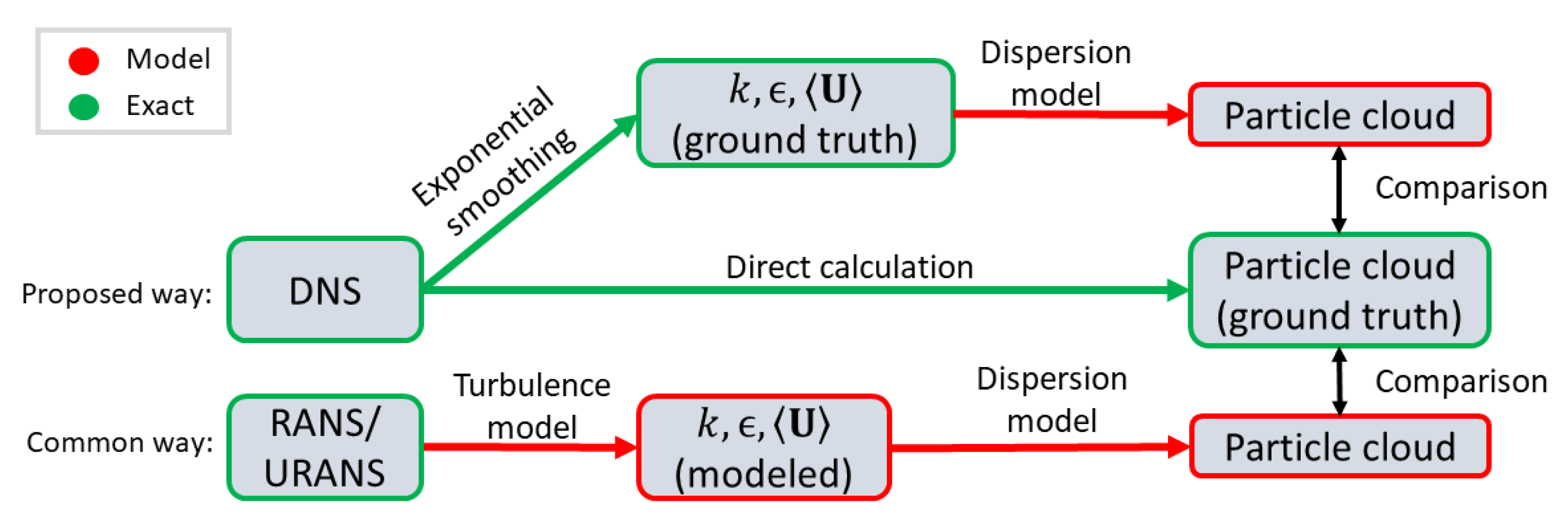
2.2. Overview of the Validation Method

The main objective of this study is to evaluate and improve stochastic particle dispersion models using DNS data. To this end, we propose a validation framework in which the fully resolved DNS velocity field is time-averaged to mimic RANS-like variables, such as the mean velocity $\langle {\mathit{U}}^n\rangle$, the turbulent kinetic energy k and the turbulent dissipation rate $ϵ$. These fields serve as input for various dispersion models, allowing direct comparison with particles solved in the DNS.

The flow chart in Figure 3 illustrates the proposed method in comparison with the conventional method. It highlights that, in the conventional approach, the input fields for the dispersion model are already approximated by a turbulence model, whereas, in the approach proposed here, they are obtained in the DNS.

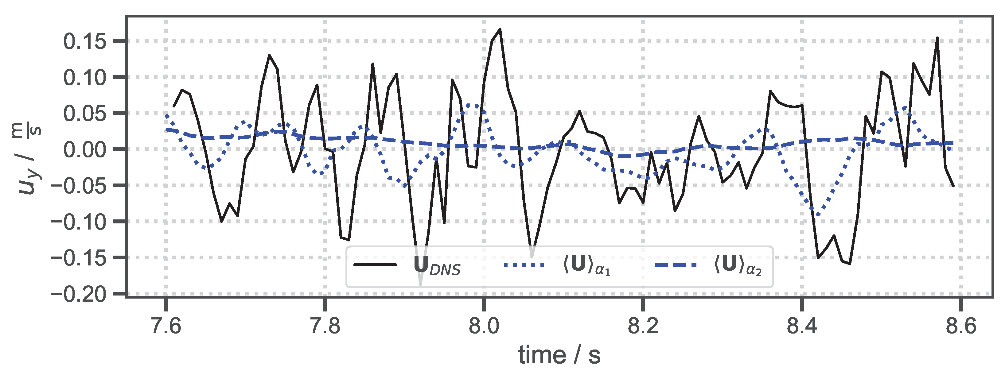
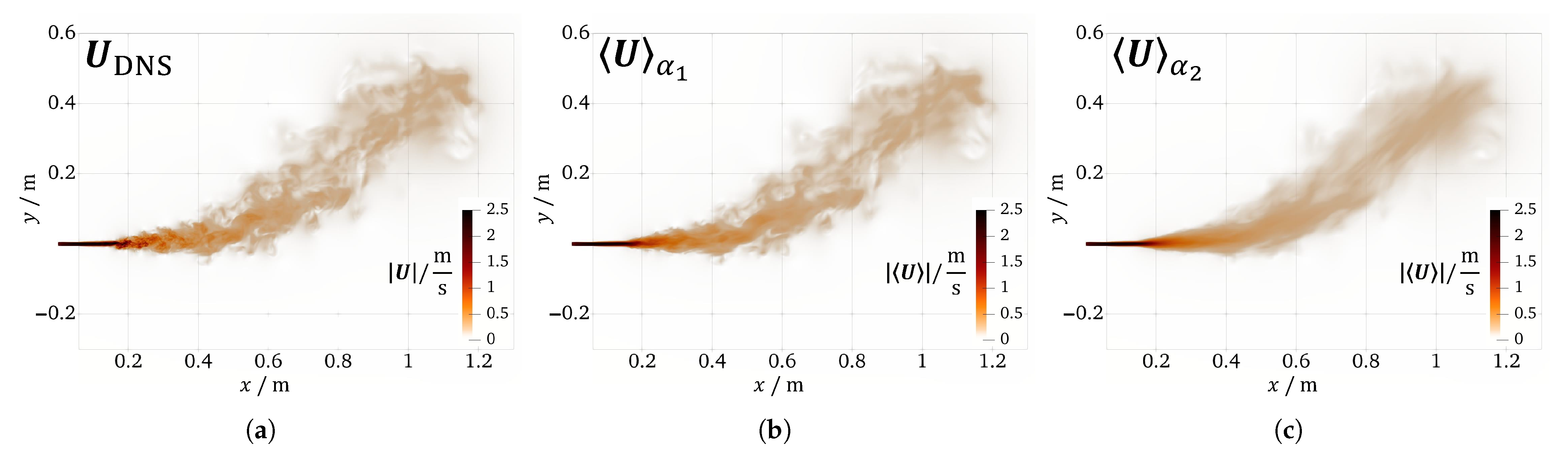
2.3. Time-Averaging of DNS Velocity Field

To provide mean flow fields and their fluctuations in the considered time-dependent flow, we apply the exponential moving average (EMA) method, also referred to as exponential smoothing, to extract the long-term mean flow variations and to explicitly filter out high-frequency fluctuations in the velocity field of the DNS. With this approach, we extract the mean velocity field and its large-scale evolution over time. Note that only the high-frequency turbulence is filtered out, while the mean flow still evolves over time in accordance with the remaining low-frequency turbulence. If $\langle {\mathit{U}}^n\rangle$ denotes the remaining mean velocity field at time n in the considered EMA method, the update of this estimated mean velocity field

$$\langle {\mathit{U}}^{n+1}\rangle =\alpha {\mathit{U}}^{n+1}+(1-\alpha )\langle {\mathit{U}}^n\rangle$$

(4)

is performed with the smoothing factor $\alpha$. As mentioned in the Introduction, the algorithm only requires the storage of $\langle {\mathit{U}}^n\rangle$, which is a significant improvement compared to a moving arithmetic average. The smoothing factor $\alpha$ controls the weighting of the current velocity and the instantaneous velocity to compute the new mean velocity. According to [9], $\alpha$ is related to the cut-off frequency ($f_c$) by

$$\alpha \simeq {\displaystyle \frac{2\pi f_c\Delta t}{\sqrt{3}}}\approx 3.628f_c\Delta t,$$

(5)

where $\Delta t$ is the time-step size of the DNS. The smallest Kolmogorov time scale is ${\tau }_{\eta }\approx 4\times {10}^{-3}$ s, which is typically an order of magnitude larger than the stability constraint imposed by the explicit time-stepping scheme (Section 2.1). Given that the jet Reynolds number of the breath is 1400, the integral turbulence time scale ${\tau }_0$ can be estimated using the Kolmogorov hypothesis as ${\tau }_0\sim {\tau }_{\eta }{\mathrm{Re}}^{1/2}$[17], yielding ${\tau }_0\sim 1.4\times {10}^{-1}$ s. This corresponds to a characteristic turbulence frequency of $1/{\tau }_0\sim 6.8$ Hz.

To investigate the effect of temporal smoothing, the following two cut-off frequencies are used for exponential averaging: 5.5 Hz and 0.55 Hz. Both are below the above-discussed characteristic turbulence frequency and differ by an order of magnitude. They correspond to smoothing factors of ${\alpha }_1=0.002$ and ${\alpha }_2=0.0002$, respectively. The corresponding time-averaged velocity fields obtained with ${\alpha }_1$ and ${\alpha }_2$ are denoted as ${\langle \mathit{U}\rangle }_{{\alpha }_1}$ and ${\langle \mathit{U}\rangle }_{{\alpha }_2}$, respectively, in the following sections. Figure 4 shows the time series of the instantaneous velocity component $U_y$ and the signals obtained by smoothing using ${\alpha }_1$ and ${\alpha }_2$. As expected, ${\langle \mathit{U}\rangle }_{{\alpha }_2}$ produces a smoother field compared to ${\langle \mathit{U}\rangle }_{{\alpha }_1}$ due to the lower cut-off frequency.

By subtracting the mean velocity vector field obtained with the EMA method from the instantaneous velocity vector field, the vector of instantaneous velocity fluctuations can be calculated as $\mathit{u}=\mathit{U}-\langle \mathit{U}\rangle$. The corresponding time-averaged kinetic energy and dissipation rate of these fluctuations are $k={\displaystyle \frac{1}{2}}\left(\langle u_x^2\rangle +\langle u_y^2\rangle +\langle u_z^2\rangle \right)$ and $ϵ=2\nu \langle {\mathcal{S}}_{ij}:{\mathcal{S}}_{ij}\rangle$, where ${\mathcal{S}}_{ij}={\displaystyle \frac{1}{2}}\left({\displaystyle \frac{\partial u_i}{\partial x_j}}+{\displaystyle \frac{\partial u_j}{\partial x_i}}\right)$ is the strain rate of the fluctuating velocity $\mathit{u}$. The terms $\langle u_x^2\rangle$, $\langle u_y^2\rangle$, $\langle u_z^2\rangle$ and $\langle {\mathcal{S}}_{ij}:{\mathcal{S}}_{ij}\rangle$ are calculated in the same way as $\langle {\mathit{U}}^{n+1}\rangle$ in Equation (4), using the EMA method and the same smoothing factor $\alpha$. These time-averaged properties of the fluctuations are used to predict the stochastic dispersion acting on the particles.

2.4. Particle Dynamics and Dispersion Models

The expiratory particles were injected randomly from a circular area with a diameter of 1 cm located at the pipe outlet at the initial velocity of the surrounding air. Particle injection started 24 s after the breathing flow was initiated to ensure that the particles entered the fully developed breathing jet rather than the quiescent surrounding air. They were injected at a constant rate of 10,000 particles per second, equally distributed over five discrete particle size bins, namely 1 $\mathrm{\mu }$m, 2 $\mathrm{\mu }$m, 4 $\mathrm{\mu }$m, 8 $\mathrm{\mu }$m and 16 $\mathrm{\mu }$m, corresponding to 2000 particles per second for each size.

The Stokes relaxation time of a single droplet is given by ${\tau }_p=d_p^2({\rho }_p-\rho )/18\nu \rho$, where $d_p$ and ${\rho }_p$ are the diameter and the density of the particle, respectively. The corresponding Stokes number St of the particle is $\mathrm{St}={\tau }_p/{\tau }_{\eta }$, as calculated in Snyder and Lumley [18]. In our study, this resulted in the smallest Stokes number ${\mathrm{St}}_1\approx 0.0008$ for a particle with a diameter of 1 $\mathrm{\mu }$m and the largest Stokes number ${\mathrm{St}}_{16}\approx 0.2$ for a particle with a diameter of 16 $\mathrm{\mu }$m in the fully resolved velocity field.

To study the particle dynamics, the expiratory particles were assumed to be discrete spherical points of constant mass. Newton’s second law of motion was applied and solved simultaneously with the flow field at each time step, taking into account both the aerodynamic drag forces ${\mathit{F}}_D$ and the gravitational forces ${\mathit{F}}_G$, as follows:

$$m_p{\displaystyle \frac{d{\mathit{U}}_p}{dt}}={\mathit{F}}_D+{\mathit{F}}_G=C_D{\displaystyle \frac{\pi d_p^2}{8}}\rho \left({\mathit{U}}_p-{\mathit{U}}_c\right)\left|{\mathit{U}}_p-{\mathit{U}}_c\right|+{\displaystyle \frac{\pi d_p^3}{6}}\left({\rho }_p-\rho \right)\mathit{g}.$$

(6)

In Equation (6), $m_p$, ${\mathit{U}}_p$, ${\rho }_p$ and $d_p$ represent the particle mass, velocity, density and diameter, respectively. The drag coefficient $C_D$ is a function of the particle Reynolds number (${\mathrm{Re}}_p$) and is given by [19]

$$C_D=\left\{\begin{array}{cc}{\displaystyle \frac{24}{{\mathrm{Re}}_p}}\left(1+{\displaystyle \frac{1}{6}}{\mathrm{Re}}_p^{2/3}\right),\hfill & \mathrm{if}{\mathrm{Re}}_p\le 1000,\hfill \\ 0.424,\hfill & \mathrm{if}{\mathrm{Re}}_p>1000,\hfill \end{array}\right.$$

(7)

where ${\mathrm{Re}}_p=d_p|{\mathit{U}}_p-{\mathit{U}}_c|/\nu$, with ${\mathit{U}}_c$ being the carrier velocity from the continuous phase—in the present case, air.

In the DNS, particles are moving within a fully resolved instantaneous turbulent velocity field $\mathit{U}$, which includes turbulent fluctuations at all scales, so no additional dispersion modeling is required. Hence, ${\mathit{U}}_c=\mathit{U}$. In contrast, when the carrier velocity field is time-averaged (e.g., $\langle \mathit{U}\rangle$), the effect of unresolved turbulence on particle motion must be modeled explicitly.

To account for the effects of unresolved turbulence on particle motion, we use a stochastic dispersion model that superimposes the vector of fluctuating velocities ${\mathit{u}}_t$ on the time-averaged velocity vector, giving ${\mathit{U}}_c=\langle \mathit{U}\rangle +{\mathit{u}}_t$. Here, the superimposed vector of velocity fluctuations determines the interaction between particles and turbulent eddies; hence, it is named the eddy interaction model (EIM). In this approach, “virtual” eddies are assumed to have a lifetime $t_e$ and a characteristic length scale ${\lambda }_e$ [4,20] and are subject to velocity fluctuations ${\mathit{u}}_t$ induced by the eddy. Assuming isotropic turbulence, ${\mathit{u}}_t$ is modeled (see, for example, [4,20,21]) as

$${\mathit{u}}_t=\sqrt{{\displaystyle \frac{2k}{3}}}\left|N\right|{\mathit{e}}_{\mathrm{dir}},$$

(8)

where N is a Gaussian random number with zero mean and unit standard deviation, and ${\mathit{e}}_{\mathrm{dir}}$ is a randomly chosen unit vector defining the direction of the velocity fluctuation vector. While ${\mathit{u}}_t$ defines the magnitude and direction of the velocity fluctuation, the eddy interaction time $t_{int}$ specifies how long the particle is affected by this modeled velocity fluctuation ${\mathit{u}}_t$ before a new ${\mathit{u}}_t$ is sampled randomly. This particle–eddy interaction ends when either the eddy lifetime $t_e$ elapses or the particle crosses the eddy in time $t_r$.

The characteristic eddy length scale ${\lambda }_e$—required to determine the interaction time between the particle and the eddy—is typically defined as

$${\lambda }_e=C_{\mu }^{3/4}{\displaystyle \frac{k^{3/2}}{ϵ}},$$

(9)

with $C_{\mu }=0.0891$ as an empirical coefficient.

In the literature [20,22,23], several eddy lifetimes are defined, all based on the eddy size ${\lambda }_e$ and the velocity fluctuations $u_t$, from which the eddy lifetime $t_e$ can be calculated (Equation (10) [5,22,23]; Equation (11) [20]):

$$t_{e,1}={\displaystyle \frac{{\lambda }_e}{\sqrt{\frac{2k}{3}}}}\stackrel{\mathrm{Equation}\left(9\right)}{=}{C}_e{\displaystyle \frac{k}{ϵ}},$$

(10)

$$t_{e,2}={\displaystyle \frac{{\lambda }_e}{|{\mathit{u}}_t|}},$$

(11)

where $C_e=C_{\mu }^{3/4}/\sqrt{2/3}$. The dispersion model implemented in OpenFOAM^® is obtained by setting $C_e=1$ in Equation (10) so that $t_{e,1}=k/ϵ$. ELT $t_{e,2}$ in Equation (11) corresponds to the eddy lifetime at the randomized fluctuating velocity vector ${\mathit{u}}_t$, while $t_{e,1}$ in Equation (10) can be interpreted as the mean eddy lifetime. Dehbi [24] used $C_e=1/7$, and Mito and Hanratty [25] found $C_e=1/21$ to be a good fit to DNS data. Although we were not able to find $C_e=1$ in the literature, we assume $C_e=1$ here because this is how it is implemented in the widely used OpenFOAM^® toolkit [5]. A more detailed overview of the used dispersion models is given in

Table 2. Overview of the different eddy interaction times used in this study.

Label	Abbreviation	Eddy Interaction Time	Used in
Mean Particle–Eddy Interaction Time	MPI	$\min (t_{e,1},t_r)$	OpenFOAM® [5]
Randomized Particle–Eddy Interaction Time	RPI	$\min (t_{e,2},t_r)$	Gosman and Ioannides [20]
Limited Particle–Eddy Interaction Time	LPI	$\min (t_{e,1},C_r{t}_{e,2},t_r)$	–

.

The following eddy crossing time is defined more consistently in the literature [4]:

$$t_r={\displaystyle \frac{{\lambda }_e}{|{\mathit{u}}_{rel}|}}=C_{\mu }^{3/4}{\displaystyle \frac{k^{3/2}}{ϵ|{\mathit{u}}_{rel}|}},\mathrm{where}|{\mathit{u}}_{rel}|=|{\mathit{U}}_c-{\mathit{U}}_p|.$$

(12)

With $t_{e,1}$ and $t_r$, the total eddy interaction time is given by

$$t_{int}=\min (t_{e,1},t_r)=\min \left({\displaystyle \frac{k}{ϵ}},{\displaystyle \frac{{\lambda }_e}{|{\mathit{u}}_{rel}|}}\right).$$

(13)

For heavy particles with large inertia and relative velocity $|{\mathit{u}}_{rel}|$, $t_r$—and, thus, the interaction time—is rather small. Small particles, on the other hand, experience longer interaction times, typically limited by $t_{e,1}$.

New Eddy Interaction Time

To overcome the overdispersion behavior of the particles, which was observed in a previous study [2] when using the eddy interaction time implemented in OpenFOAM^® (Equation (10)), we propose to modify the eddy interaction time by introducing an additional constraint on it:

$$t_{int,new}=\min \left(t_{e,1},C_r{t}_{e,2},t_r\right)=\min \left({\displaystyle \frac{k}{ϵ}},C_r{\displaystyle \frac{{\lambda }_e}{|{\mathit{u}}_t|}},{\displaystyle \frac{{\lambda }_e}{|{\mathit{u}}_{rel}|}}\right),$$

(14)

where the additional constraint $C_r{t}_{e,2}$ in Equation (14) limits the maximum displacement of a particle within a single eddy to the optimum of $C_r=16$ times the amount of time that a particle needs to pass the eddy’s characteristic length ${\lambda }_e$, i.e., the size of the eddy, with the randomized fluctuation velocity. Therefore, if the random $|{\mathit{u}}_t|$ is large, $t_{e,2}$ becomes small. This effectively limits the displacement. Conversely, if the random $|{\mathit{u}}_t|$ is small, using $t_{e,2}$ alone could lead to unreasonably long interaction times. Note that $C_r=16$ is the optimal value for breathing, which was determined by varying $C_r$ from 1 to infinity. Thus, instead of replacing the eddy lifetime $t_{e,1}$ (as in the RPI model; see Table 2), we introduce $t_{e,2}$ as an additional boundary to limit the displacement while maintaining realistic interaction times for eddies with slow perturbation velocities. Although $t_{e,2}$ has been introduced as an eddy lifetime formulation [20], we use it as a selective displacement limiter for large ${\mathit{u}}_t$.

Table 2 provides an overview of the eddy interaction times used in this study: the mean particle-eddy interaction time (MPI), which is available in OpenFOAM^®; the randomized particle-eddy interaction time (RPI), which is based on an eddy lifetime and the randomized fluctuating velocity vector ${\mathit{u}}_t$; and the new model using the limited particle–eddy interaction time (LPI), which stops the interaction between the particle and the eddy once the particle has been displaced with respect to the eddy’s length.

2.5. Test Cases

To evaluate the effect of dispersion modeling on particle motion, a comparative analysis was carried out for nine clouds with particles of different sizes. The development of these clouds was computed in a reference DNS and by solving Equation (6) with the mean DNS flow fields.

For each mean velocity field ${\langle \mathit{U}\rangle }_{{\alpha }_1}$ and ${\langle \mathit{U}\rangle }_{{\alpha }_2}$ obtained from the two smoothing factors ${\alpha }_1$ and ${\alpha }_2$, we analyzed and compared the different stochastic particle dispersion models (MPI, RPI) and the new limited particle–eddy interaction time (LPI) model described in Section 2.4. Moreover, in order to highlight the effect of a dispersion model, the particle dispersion induced by the mean flow field without a dispersion model was computed for comparison.

The particle dispersion analysis of the particles resolved in the mean velocitcy field ${\langle \mathit{U}\rangle }_{{\alpha }_1}$ is not shown, as the filtering effect is negligible and a particle dispersion model is not necessary (see Section 3.1). Therefore, we focus only on the simulated particle clouds using the mean velocity field ${\langle \mathit{U}\rangle }_{{\alpha }_2}$ to evaluate the performance of the PDMs discussed above. A detailed overview of the predicted particle clouds is given in

Table 3. Overview of the tested particle clouds with varying configurations.

Particle Cloud	Velocity Field	Cut-Off Frequency	Dispersion Model	Particle–Eddy Interaction Time
1	DNS	−	−	−
2	${\langle \mathit{U}\rangle }_{{\alpha }_2}$	0.55 Hz	−	−
3	${\langle \mathit{U}\rangle }_{{\alpha }_2}$	0.55 Hz	MPI	$\min (t_{e,1},t_r)$
4	${\langle \mathit{U}\rangle }_{{\alpha }_2}$	0.55 Hz	RPI	$\min (t_{e,2},t_r)$
5	${\langle \mathit{U}\rangle }_{{\alpha }_2}$	0.55 Hz	LPI	$\min (t_{e,1},C_r{t}_{e,2},t_r)$

.

2.6. Evaluation Methods for Particle Dispersion

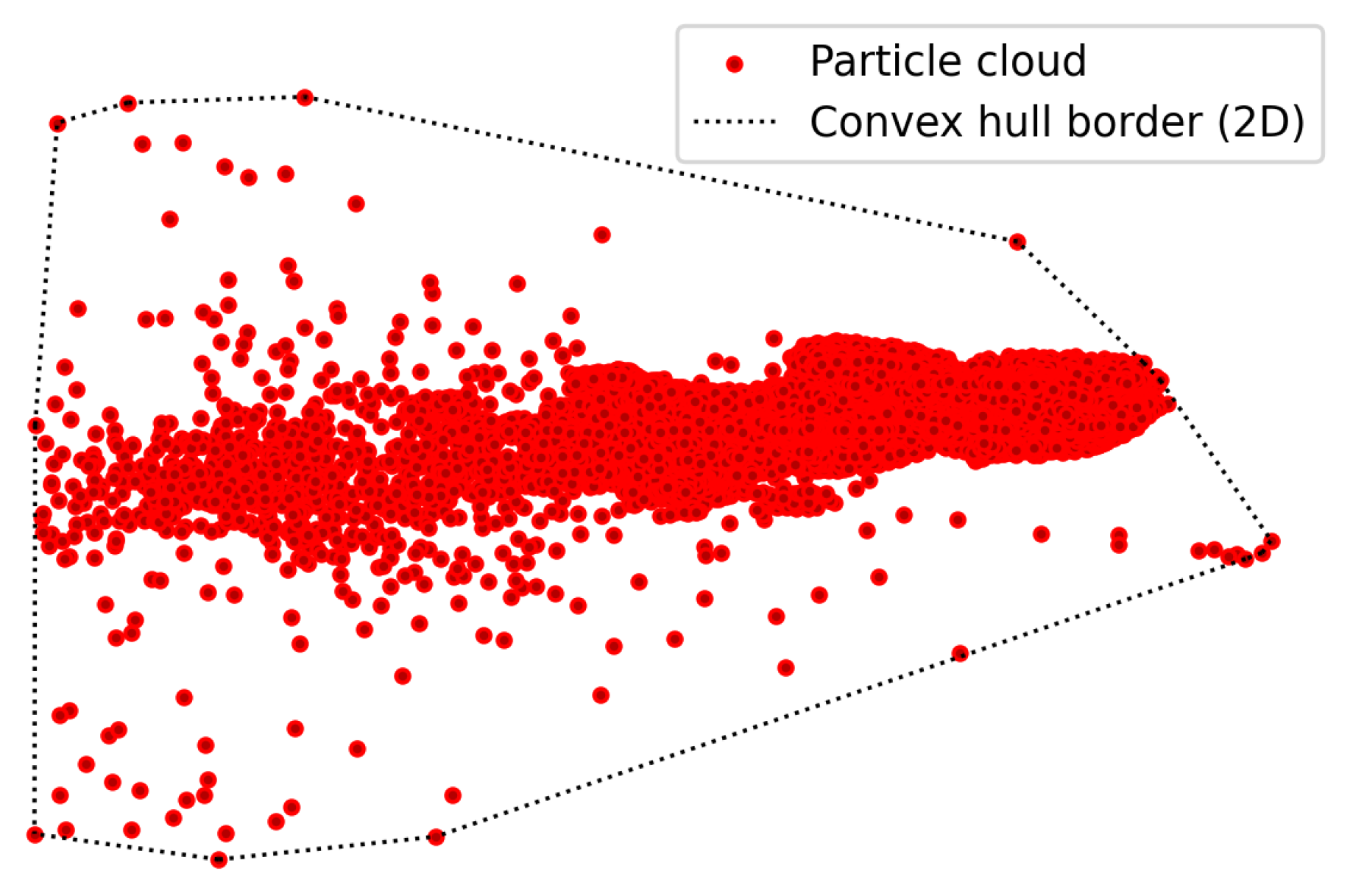
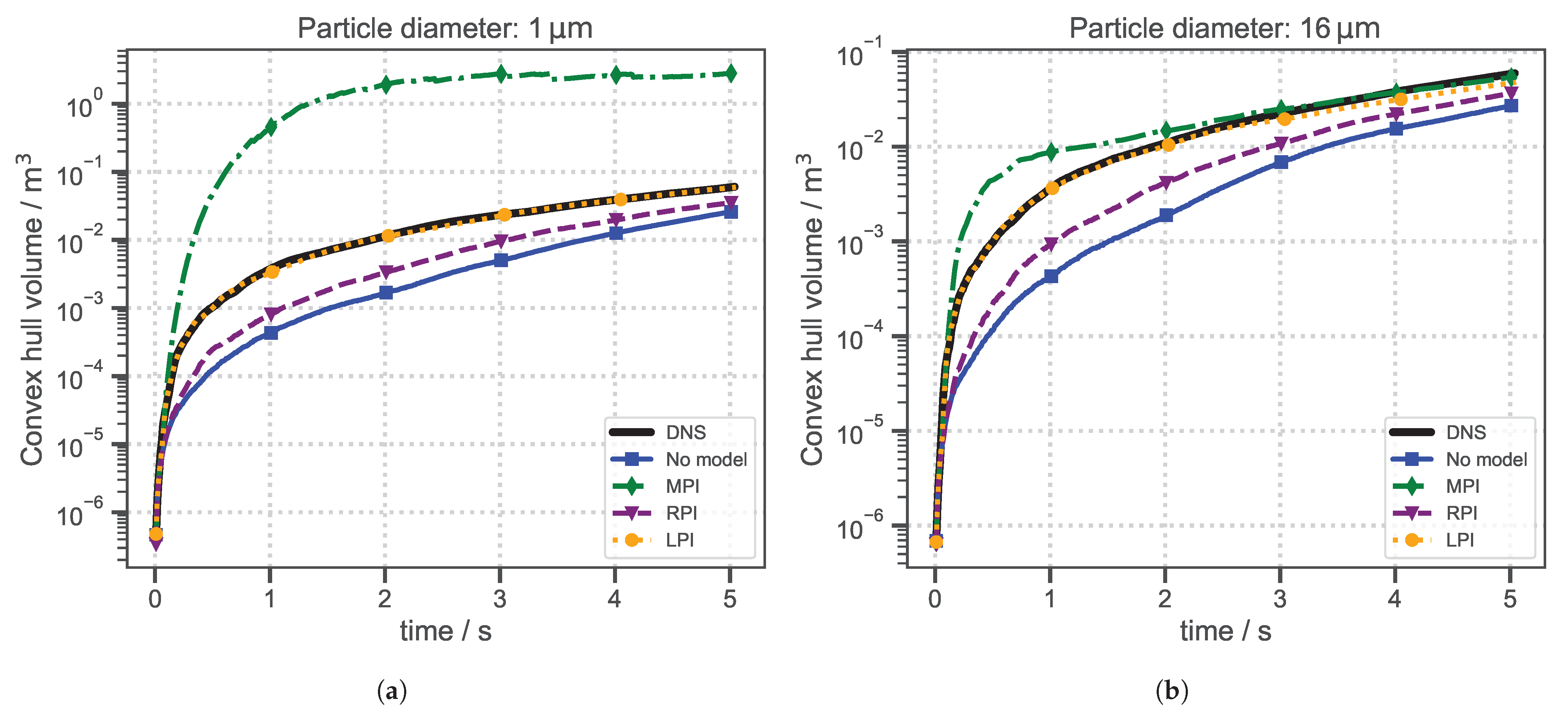
To demonstrate the performance of the new model (LPI) in comparison with the dispersion model using the mean particle–eddy interaction time (MPI), the modeled particle dispersions were analyzed in three ways. The first method is to determine the convex hull, which is the maximum particle cloud volume. The second method is to use the mean square distance $D^2$ as a measure of the dispersion within the particle cloud, and the third method is based on the particle concentration.

2.6.1. Convex Hull

The convex hull is the smallest possible shape that contains all particles where all interior angles are convex (<180°), as shown in Figure 5. It can be seen that the shape of the convex hull is determined by a small fraction of the particles, while the majority of the particles within the hull have no influence on the shape. Therefore, this method makes the most “extreme” particles visible. In 2D, each line segment connects two points/particles. We applied the same concept to the 3D cloud, with three particles spanning a triangular surface. The convex hull volume can be interpreted as the “contaminated” volume where interactions with particles are possible.

2.6.2. Mean Square Distance $D^2$

Since the convex hull only captures the behavior of outlier particles, we also computed the mean squared distance of all possible particle pairs using the $D^2$ method:

$$\begin{array}{cc}\hfill D^2& ={\displaystyle \frac{1}{N_d}}\sum _{i,j=0}^{N_p}{({\mathit{X}}_i-{\mathit{X}}_j)}^2,\hfill \end{array}$$

(15)

$$\begin{array}{cc}\hfill N_d& =N_p(N_p-1),\hfill \end{array}$$

(16)

where $N_d$ is the number of possible distances between the number of particles $N_p$, and ${\mathit{X}}_i$ and ${\mathit{X}}_j$ indicate the positions of the particles. This method provides insight into the general dispersion of the cloud and is not dominated by individual outlier particles.

2.6.3. Particle Concentration

Although the $D^2$ method takes the entire cloud into account, it represents the cloud as a single scalar value and does not provide information on how the particles are distributed within the cloud. Therefore, as a third measure, we chose to evaluate the particle concentration at different distances from the center of the breathing jet. Since the particle concentrations must be averaged over a volume, a ring-shaped volume $V_r$ around the breathing jet at a distance $x_r=0.8$m from the mouth was selected, as shown in Figure 6.

We increased the radius $r_r$ in incremental steps to obtain the particle concentrations at any distance from the jet. The particle concentration in the ring was calculated by

$$\begin{array}{cc}\hfill C_r& ={\displaystyle \frac{N_V}{V_r}},\hfill \end{array}$$

(17)

$$\begin{array}{cc}\hfill V_r& =\pi ({(r_r+{\displaystyle \frac{\Delta r_r}{2}})}^2-{(r_r-{\displaystyle \frac{\Delta r_r}{2}})}^2)\Delta x_r,\hfill \end{array}$$

(18)

where $N_V$ represents the number of particles in the ring-shaped volume $V_r$, $\Delta x=4$cm is the width of the ring in the streamwise direction, and $r_r$ and $\Delta r_r=3$ cm indicate the radius and radial thickness, respectively. This allows us to analyze the particle distribution around the jet.

3. Results and Discussion

In Section 3.1, the resulting mean velocity fields obtained with different smoothing factors (${\alpha }_1$ and ${\alpha }_2$) are discussed. Subsequently, in Section 3.2, the main results of our study are presented: a comparison of the particle dispersion based on different modeling approaches.

3.1. Comparison of Mean Velocity Fields

For the validation of the particle dispersion models, we applied strong (${\alpha }_2$) and weak (${\alpha }_1$) exponential smoothing (see Section 2.3) to the turbulent DNS velocity field to obtain the running mean velocity components of the DNS. Figure 7a shows the DNS velocity field at $t=10$ s, while the corresponding mean velocity fields ${\langle \mathit{U}\rangle }_{{\alpha }_1}$ and ${\langle \mathit{U}\rangle }_{{\alpha }_2}$ are shown in Figure 7b,c.

The mean velocity field ${\langle \mathit{U}\rangle }_{{\alpha }_1}$ in Figure 7b is very similar to the DNS velocity field for $x>0.4$ m, i. e., in the downstream region where the jet momentum has partially dissipated and buoyancy effects are noticeable. In contrast, the mean velocity field ${\langle \mathit{U}\rangle }_{{\alpha }_2}$(Figure 7c) shows a much smoother velocity field compared to the DNS velocity field throughout the flow, highlighting the stronger smoothing effect of ${\alpha }_2$.

Figure 8a shows the smallest (1 $\mathrm{\mu }$m) and the largest (16 $\mathrm{\mu }$m) particle clouds predicted by the DNS, while Figure 8b,c show the particle clouds predicted in the velocity fields ${\langle \mathit{U}\rangle }_{{\alpha }_1}$ and ${\langle \mathit{U}\rangle }_{{\alpha }_2}$, without additional dispersion models. The particle clouds predicted in the DNS and ${\langle \mathit{U}\rangle }_{{\alpha }_1}$ look almost the same, indicating that ${\langle \mathit{U}\rangle }_{{\alpha }_1}$ still contains a relevant amount of turbulence in the smoothed part of the velocity field. This shows that an additional dispersion model is not required to correctly estimate the particle tracks. However, the particle cloud predicted in ${\langle \mathit{U}\rangle }_{{\alpha }_2}$ (Figure 8c) has less dispersion compared to the prediction obtained from the DNS, highlighting the need to model turbulent dispersion in order to reduce the dispersion error.

Based on the observations obtained when comparing the mean velocity fields and the particle clouds predicted in ${\langle \mathit{U}\rangle }_{{\alpha }_1}$ and ${\langle \mathit{U}\rangle }_{{\alpha }_2}$ with those of the DNS, we choose not to show the dispersion models’ performance in terms of ${\langle \mathit{U}\rangle }_{{\alpha }_1}$ due to its similarity to the case of the DNS. Hence, in the next section, we only evaluate the particle clouds predicted in ${\langle \mathit{U}\rangle }_{{\alpha }_2}$ using the three dispersion models (see Table 2), as well as those simulated with the DNS velocity field and without applying any dispersion model.

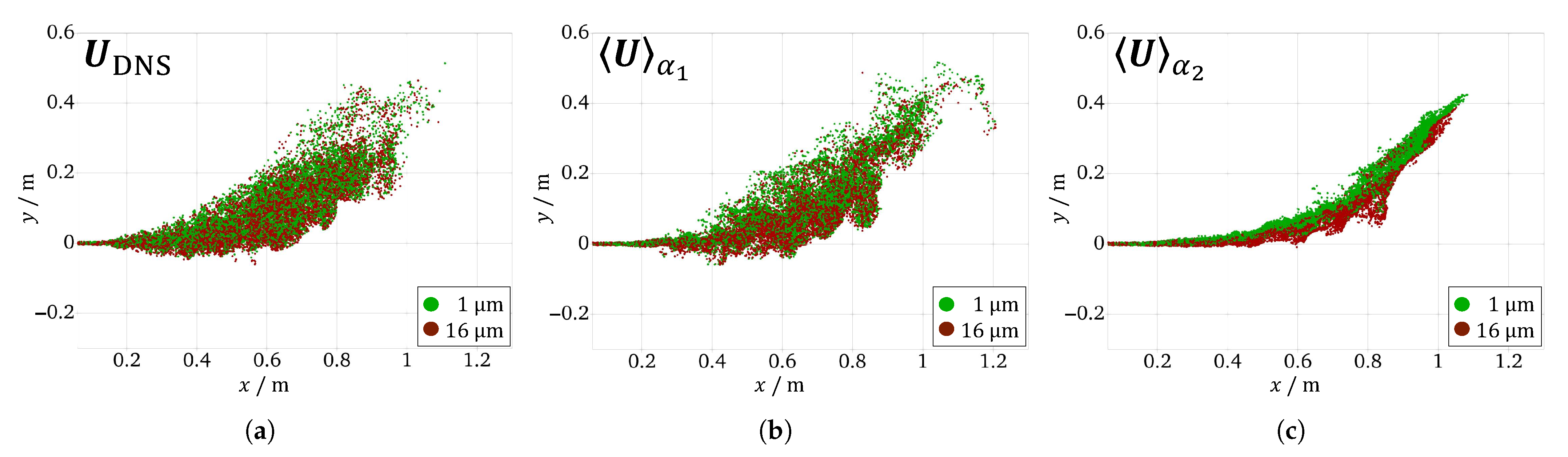
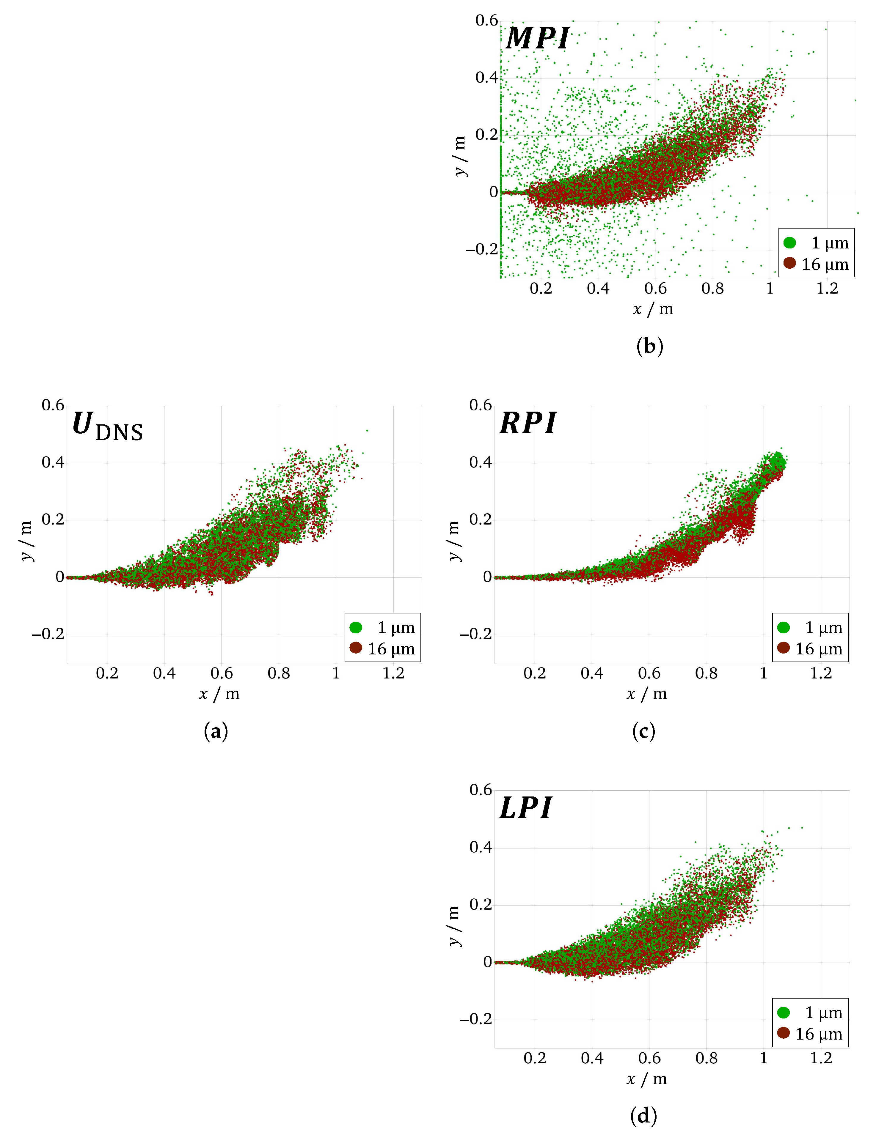
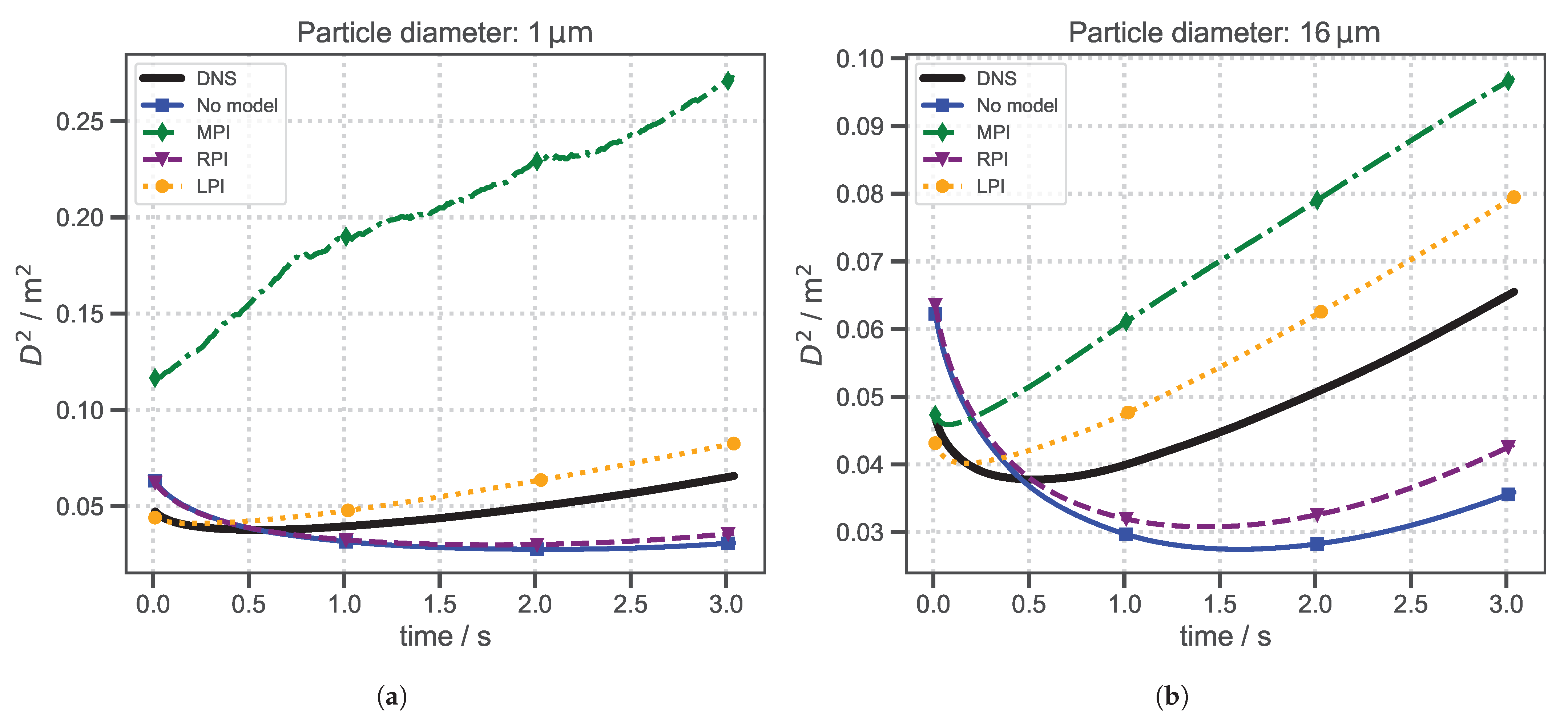
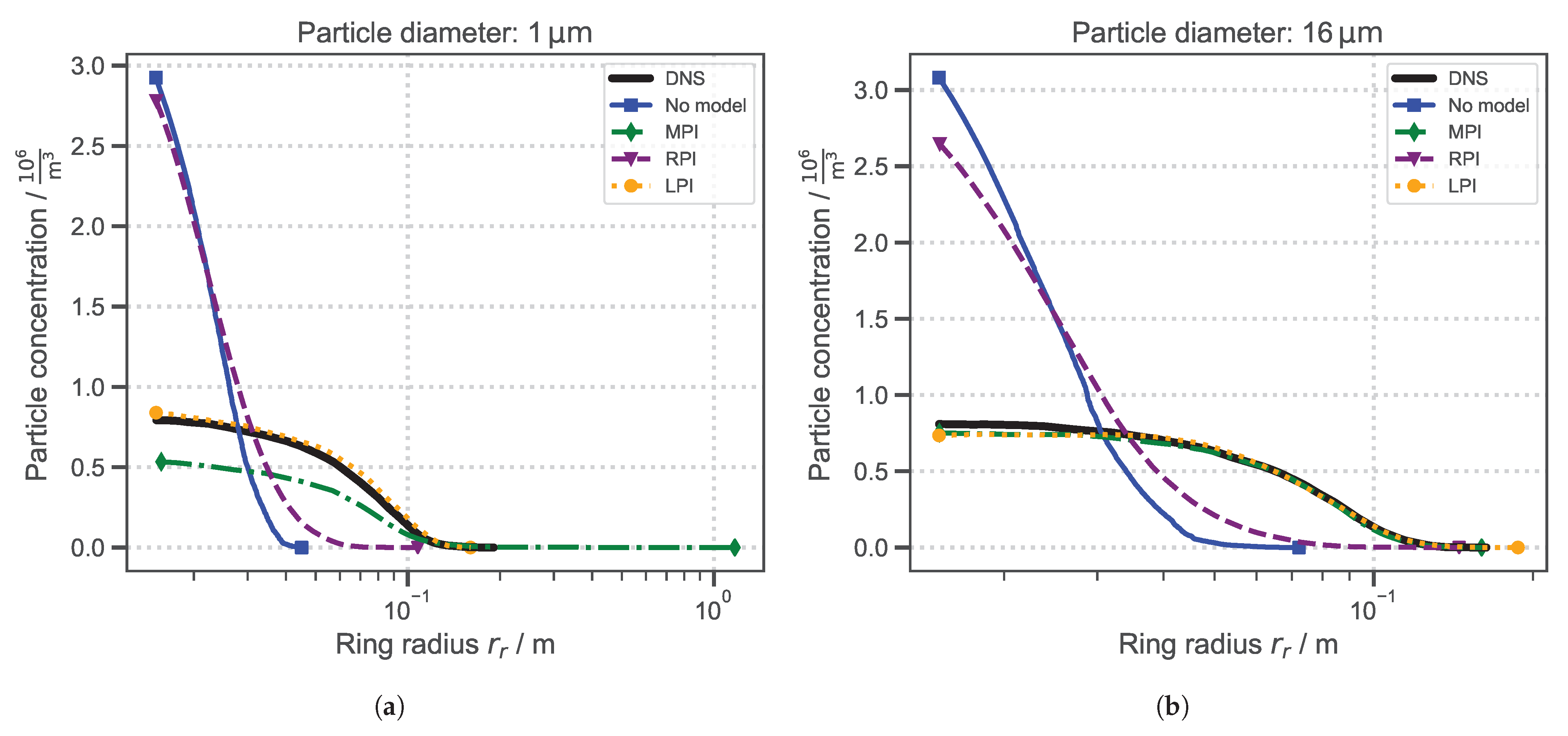
3.2. Comparison of Particle Dispersion

At the beginning of this section, a brief overview of the particle clouds predicted by different dispersion models, focusing only on the smallest (1 $\mathrm{\mu }$m) and the largest (16 $\mathrm{\mu }$m) particle sizes, is provided. Further, the particle dispersion resulting from different particle dispersion modeling approaches applied to the mean velocity field is evaluated and compared to the DNS results using three evaluation metrics: the convex hull volume (CHV), the mean square distance ($D^2$) and the particle concentration. In addition, these evaluation metrics are applied to the particle dispersion in the mean velocity field without a dispersion model in order to demonstrate the absolute improvement provided by the dispersion model regarding particle dispersion. Finally, the particle clouds with different particle sizes (1 $\mathrm{\mu }$m, 2 $\mathrm{\mu }$m, 4 $\mathrm{\mu }$m, 8 $\mathrm{\mu }$m, 16 $\mathrm{\mu }$m) are compared by determining the root mean square errors (RMSEs) of the particle dispersions evaluated by the CHV, $D^2$ and particle concentration methods compared to the DNS.

Figure 9 shows the particle clouds predicted in the DNS (Figure 9a) and those predicted with the MPI model (Figure 9b), the RPI model (Figure 9c), and the LPI model (Figure 9d). Compared to the particle cloud obtained in the DNS, the particle cloud predicted with the MPI model exhibits erratic particle dispersion when it comes to small particles, while the large particles (16 $\mathrm{\mu }$m) remain within the jet flow, where the eddy interaction is terminated by the particle crossing time $t_r$, rather than by the eddy lifetime. As discussed in Section 2.4, the reason for this non-physical behavior predicted for the small particles is that the eddy interaction time is not determined by the randomized velocity fluctuation ${\mathit{u}}_t$ that the particle actually experiences, but with the mean absolute $\langle \left|{\mathit{u}}_t\right|\rangle$. Consequently, any particle that randomly samples a particularly high ${\mathit{u}}_t$ will receive the same eddy interaction time as any other particle and can thus travel several decimeters before the eddy lifetime expires.

To overcome this problem, we propose to limit the eddy interaction time (see Section 2.4). In contrast to the MPI model, the RPI model suppresses the erratic particle motion. However, the resulting particle cloud is more confined than the cloud obtained in the DNS. The cloud obtained with the LPI model achieves the desired outcome, similar to the MPI model, but without the individual unrealistically dispersed particles.

Figure 10a,b show the evolution of the convex hull volume (CHV; see Section 2.6.1) over time for the particle clouds with the smallest (1 $\mathrm{\mu }$m) and the largest (16 $\mathrm{\mu }$m) particle sizes. All particles present in the domain are considered, regardless of their injection time. As expected, all five clouds show an increasing trend in the CHV as the particles move through the domain and progressively convect and disperse. The CHV of the particles without a particle dispersion model (No PDM) is underpredicted compared to the DNS cloud for both particle sizes. The MPI model significantly overpredicts the CHV of the small particles, resulting in values that are an order of magnitude higher than the CHV obtained from the DNS. This is caused by the erratic particle motion predicted by the MPI model, as shown in Figure 9b.

In contrast to the MPI model, the RPI model stops this erratic behavior for both particle sizes and slightly underpredicts the CHV, especially for the small particles. The proposed LPI model, on the other hand, significantly improves the accuracy of the CHV predictions, achieving near-perfect agreement with the DNS results for both particle sizes. This makes it the most accurate dispersion model for this evaluation method. This shows that limiting the particle–eddy interaction time in the MPI model has the intended effect of reducing overdispersion.

For the larger particles (16 $\mathrm{\mu }$m), the observations are very similar to those for the small particles for the RPI and LPI models, except that the erratic motion of the particles computed with the MPI model disappears, showing reasonably better performance. Since the eddy interaction time for larger particles is more likely to be determined by the particle crossing time than by the eddy lifetime, and since all three dispersion models use exactly the same particle crossing time, it is expected that the models will produce similar results for large particles.

As the CHV is only determined by the outermost particles, it provides insight into the extent of the most widely dispersed particles. However, it does not fully characterize the dispersion of the entire particle cloud. Therefore, we also analyzed the mean square distance $D^2$ of these clouds separately for the small (Figure 11a) and large (Figure 11b) particles released over the course of 2 s.

The $D^2$ of the cloud predicted without a PDM is underpredicted compared to the cloud predicted by the DNS for both particle sizes, showing that a PDM is required to predict the correct $D^2$. Using the RPI model results in a small improvement for the large (16 $\mathrm{\mu }$m) particles, but no significant improvement for the small (1 $\mathrm{\mu }$m) particles is achieved. In contrast, the LPI model predicts $D^2$ values that are significantly closer to those predicted by the DNS for both particle sizes. The MPI model, on the other hand, results in significant overprediction for both particle sizes—even more so for small particles—compared to the DNS results.

Overall, the $D^2$ analysis confirms the results of the convex hull volume analysis: the MPI model significantly overpredicts the particle dispersion, while the LPI model suppresses erratic particle motion and results in better agreement with the DNS. Although the mean square distance $D^2$ is evaluated with all particles in the cloud, it provides only limited insight into the internal distribution of the particles. Therefore, Figure 12 plots the time-averaged particle concentration as a function of the radial distance from the jet center (see Figure 6) for 1 $\mathrm{\mu }$m particles (a) and 16 $\mathrm{\mu }$m particles (b), measured at a downstream position of 0.8 m from the jet outlet. The x-axis is plotted on a logarithmic scale. All models show a decreasing trend for both particle sizes, indicating that the highest particle concentration occurs at the jet center in each cloud.

Without a PDM, the predicted particle concentration near the jet center (ring radius → 0 m) is significantly higher than the particle concentration predicted in the DNS. This suggests that dispersion models are needed to improve the dispersion away from the jet center. Although the RPI model provides an improvement for the large particles (16 $\mathrm{\mu }$m), it does not provide an improvment over the cloud obtained without a dispersion model for the small particles (1 $\mathrm{\mu }$m); in both cases, the particle concentration decreases sharply beyond a radius of 10 cm, indicating insufficient dispersion compared to the DNS results. The LPI model significantly improves the predicted dispersion by moving the particles further away from the jet center, almost exactly matching the DNS predictions for both particle sizes. For the small particles (1 $\mathrm{\mu }$m), the MPI underpredicts the particle concentration for all radial distances compared to the DNS results. This indicates that overdispersion upstream of the location where the particle concentration is assessed ($x=0.8$m) results in fewer particles reaching the location of the particle concentration evaluation. In contrast, the MPI, like the LPI, agrees almost exactly with the DNS results for the large particles (16 $\mathrm{\mu }$m).

This analysis provides a more nuanced view of particle dispersion. It shows that the excessive early dispersion of small particles (1 $\mathrm{\mu }$m) predicted by the MPI model (upstream of $x=0.8$ m) leads to noticebly lower particle concentrations downstream than predicted by the DNS. This highlights the cumulative effect of overdispersion on downstream predictions. The RPI model falls short in improving the dispersion compared to the cases where no PDM is used. In contrast, the overdispersion and therefore the loss of particles upstream is suppressed with the LPI model, resulting in particle concentrations that are in excellent agreement with those obtained in the DNS.

In the evaluations above, we compared particle clouds for diameters of 1 and 16 $\mathrm{\mu }$m. Figure 13a extends this analysis by comparing the root mean square error (RMSE) between the convex hull volume time series of each model and the DNS for particle diameters of 1, 2, 4, 8, and 16 $\mathrm{\mu }$m. These sizes correspond to Stokes numbers (St) ranging from 0.0008 to 0.2.

The MPI model shows a strong diameter dependence: for small particles (≤$8\mathrm{\mu }$m), the RMSE is orders of magnitude higher than without using a PDM. In contrast, for large particles (16 $\mathrm{\mu }$m), the RMSE obtained with the MPI model is low and the model performs better than if no model were used.

In contrast, the RPI model slightly reduces the RMSE compared to not using a PDM for all diameters. The results obtained with the LPI model yield an even lower RMSE than the RPI model for all diameters. For 16 $\mathrm{\mu }$m particles, the smallest errors are obtained with the MPI and LPI models. Since the MPI and LPI models assume different eddy lifetimes but the same eddy crossing time, this indicates that, for the largest particles (16 $\mathrm{\mu }$m), the eddy crossing time determines the eddy interaction time.

Figure 13b presents a complementary analysis showing the RMSE of the mean square distance $D^2$ of the particle clouds obtained with the different models, namely MPI, RPI, and LPI, and without a PDM. The observed trends are consistent with the RMSE analysis of the convex hull volume: for small diameters (≤8 $\mathrm{\mu }$m), the MPI model achieves RMSE values that are significantly higher compared to the results obtained without a PDM. For the largest particles (16 $\mathrm{\mu }$m), the RMSE of the MPI model nearly reaches the values obtained without a PDM, but it still results in a higher RMSE.

On the other hand, the RMSE obtained with the RPI model is similar to that obtained without a PDM for particles with a diameter smaller than 8 $\mathrm{\mu }$m, and it is slightly lower for the particles with a diameter of 16 $\mathrm{\mu }$m. In contrast, the smallest RMSE values for all diameters are obtained using the LPI model.

Figure 13c shows the RMSE of the time-averaged particle concentration for the same set of particle clouds. In this evaluation, not using a PDM results in the highest RMSE for all diameters. The results predicted with the RPI model are only slightly more accurate compared to the case without a PDM, and the RMSE values obtained using the MPI model are significantly lower for all particle diameters, especially for the largest (16 $\mathrm{\mu }$m) particles, for which the RMSE is nearly zero. However, the LPI model results in a further significant reduction in the RMSE for particles smaller than or equal to 8 $\mathrm{\mu }$m compared to the MPI model.

Overall, these results suggest that the MPI dispersion model implemented in OpenFOAM^® is likely to significantly overpredict the dispersion of small particles in highly turbulent regions. This results directly in excessive CHV and $D^2$ values and indirectly causes excessively low particle concentrations downstream, because the overly dispersed particles are “lost” upstream.

By suppressing the erratic particle dispersion of small particles, the new model (LPI) yields the lowest RMSEs in the convex hull, mean square distance, and particle concentration analyses, making it a promising alternative. This suggests that, while the MPI model generally provides accurate predictions for most particles, its overall accuracy is reduced by the unrealistic trajectories of individual particles. The LPI model addresses this issue by introducing a constraint on the particle–eddy interaction time, which effectively suppresses these unrealistic trajectories.

Across all three evaluation methods (CHV, $D^2$, and particle concentration), the predictions obtained with the MPI model are significantly more accurate for 16 $\mathrm{\mu }$m particles than for 8 $\mathrm{\mu }$m particles. This suggests that the transition between eddy lifetime-dominated and eddy crossing time-dominated interaction occurs with the range of Stokes numbers between 0.05 and 0.2 for the investigated breathing flow field.

It should be noted that validation studies are often based on experimental data, e.g., in the study by Snyder and Lumley [18], where the reported minimum Stokes number is 0.145. Therefore, when applying the MPI model to the low Stokes numbers studied by Snyder and Lumley, the occurence of erratic particle trajectories is unlikely. Similarly, the Stokes numbers used in the study by Zhang et al. [6] were also too high to capture this effect. Consequently, the MPI model can accurately predict the CHV and $D^2$ of a particle cloud at the Stokes numbers used by Snyder and Lumley [18] or Zhang et al. [6]. However, our study includes Stokes numbers as low as 0.0008 (1 $\mathrm{\mu }$m particles), reflecting smaller particle sizes and flow conditions typical of human breathing. These particles (especially <5 $\mathrm{\mu }$m) are highly relevant for the transmission of infectious viruses [26,27].

This emphasizes the value of the DNS-based validation approach presented here: it allows for the evaluation of arbitrary particle sizes and flow conditions beyond the constraints of experimental setups (e.g., limitations in capturing small particles on camera). The inherent advantages of computational fluid dynamics—such as the ability to track the exact position of each particle at any point in time—allow for detailed dispersion analyses using metrics such as the convex hull volume, mean square distance $D^2$, and spatial particle concentration. Since the dispersion models all use velocity fields derived directly from the DNS, any differences in the resulting particle clouds can only be attributed to the performance of the respective dispersion model.

Based on the observations described above, we draw the following conclusions.

• Exponential smoothing is a viable, memory-efficient alternative to the conventional running average when processing DNS fields.
• Applying particle dispersion models to time-averaged DNS flow fields allows independent validation, free from secondary errors introduced by turbulence modeling or measurement uncertainty.
• The exponential smoothing approach allows us to validate arbitrary particle sizes under arbitrary flow conditions, overcoming the limitations of typical experimental setups.
• The particle dispersion model currently implemented in OpenFOAM^® (MPI) performs satisfactorily for larger particles (≥16$16\mathrm{\mu }$m, $\mathrm{St}\ge 0.2$). However, it shows erratic behavior for smaller diameters. This may be due to a lack of validation at low Stokes numbers—especially those relevant for virus-laden aerosols.
• The proposed model with the limited eddy interaction time (LPI) successfully suppresses erratic particle trajectories and outperforms both the randomized particle–eddy interaction time (RPI) and the mean particle–eddy interaction time (MPI) models in any of the dispersion evaluation methods applied. Due to its straightforward implementation and proven effectiveness in the turbulent jet configuration, this model could be particularly useful for researchers investigating particle-laden flows in respiratory or similar jet-like applications.

3.3. Limitations and Assumptions

In order to be able to isolate the effects of the turbulence kinetic energy and the turbulence dissipation rate in the particle dispersion model on particle motion, other parameters like aerosol evaporation are neglected in this study, since solving particle trajectories in either an instantaneous DNS velocity field or a mean velocity field can impact the evaporation times and, consequently, the particle dynamics [3]. Furthermore, to evaluate the performance of dispersion models for different particle sizes, the same Stokes drag model is applied to all particles. Although the Cunningham correction factor may be relevant for smaller particles, it is omitted here to ensure consistency in model evaluation.

Although turbulence in the exhaled breath jet is observed to be non-homogeneous and anisotropic, only isotropic turbulence-based particle dispersion models are applied in this study. These models are primarily designed for RANS/URANS simulations that use eddy–viscosity turbulence models, and they inherently assume isotropic turbulence. Additionally, a steady flow rate is assumed for the exhaled breath to enable temporal exponential smoothing, even though natural exhalation involves flow rate variations with typical periodicity of 2–3 s [14].

References

1. Dupont, S.; Brunet, Y.; Jarosz, N. Eulerian modelling of pollen dispersal over heterogeneous vegetation canopies. Agric. For. Meteorol. 2006, 141, 82–104. [Google Scholar] [CrossRef]
2. Batmaz, E.; Schmeling, D.; Wagner, C. DNS–URANS comparison study on cough-induced flow and particles in a large-scale circulation. Int. J. Numer. Methods Heat Fluid Flow, 2025. [Google Scholar] [CrossRef]
3. Rosti, M.E.; Cavaiola, M.; Olivieri, S.; Seminara, A.; Mazzino, A. Turbulence role in the fate of virus-containing droplets in violent expiratory events. Phys. Rev. Res. 2021, 3, 013091. [Google Scholar] [CrossRef]
4. Huilier, D.G.F. An Overview of the Lagrangian Dispersion Modeling of Heavy Particles in Homogeneous Isotropic Turbulence and Considerations on Related LES Simulations. Fluids 2021, 6, 145. [Google Scholar] [CrossRef]
5. API Guide: OpenFOAM® v2406. Available online: https://api.openfoam.com/2406/ (accessed on 17 March 2025).
6. Zhang, X.; Tian, Z.F.; Chinnici, A.; Zhou, H.; Nathan, G.J.; Chin, R.C. Particle dispersion model for RANS simulations of particle-laden jet flows, incorporating Stokes number effects. Adv. Powder Technol. 2024, 35, 104345. [Google Scholar] [CrossRef]
7. Gardner, E.S. Exponential smoothing: The state of the art. J. Forecast. 1985, 4, 1–28. [Google Scholar] [CrossRef]
8. Gardner, E.S. Exponential smoothing: The state of the art—Part II. Int. J. Forecast. 2006, 22, 637–666. [Google Scholar] [CrossRef]
9. Cahuzac, A.; Boudet, J.; Borgnat, P.; Lévêque, E. Smoothing algorithms for mean-flow extraction in large-eddy simulation of complex turbulent flows. Phys. Fluids 2010, 22, 125104. [Google Scholar] [CrossRef]
10. Gray, D.D.; Giorgini, A. The validity of the boussinesq approximation for liquids and gases. Int. J. Heat Mass Transf. 1976, 19, 545–551. [Google Scholar] [CrossRef]
11. Chorin, A.J. Numerical Solution of the Navier-Stokes Equations. Math. Comput. 1968, 22, 745–762. [Google Scholar] [CrossRef]
12. Kath, C.; Wagner, C. Highly Resolved Simulations of Turbulent Mixed Convection in a Vertical Plane Channel. New Results Numer. Exp. Fluid Mech. X 2016, 132, 515–524. [Google Scholar] [CrossRef]
13. Shishkina, O.; Wagner, C. Stability conditions for the Leapfrog-Euler scheme with central spatial discretization of any order. Appl. Numer. Anal. Comput. Math. 2004, 1, 315–326. [Google Scholar] [CrossRef]
14. Gupta, J.K.; Lin, C.H.; Chen, Q. Characterizing exhaled airflow from breathing and talking. Indoor Air 2010, 20, 31–39. [Google Scholar] [CrossRef]
15. Dekker, E. Transition between laminar and turbulent flow in human trachea. J. Appl. Physiol. 1961, 16, 1060–1064. [Google Scholar] [CrossRef]
16. Poletto, R.; Craft, T.; Revell, A. A New Divergence Free Synthetic Eddy Method for the Reproduction of Inlet Flow Conditions for LES. Flow, Turbul. Combust. 2013, 91, 519–539. [Google Scholar] [CrossRef]
17. Pope, S.B. Turbulent Flows; Cambridge University Press: Cambridge, UK, 2000. [Google Scholar] [CrossRef]
18. Snyder, W.H.; Lumley, J.L. Some measurements of particle velocity autocorrelation functions in a turbulent flow. J. Fluid Mech. 1971, 48, 41–71. [Google Scholar] [CrossRef]
19. Amsden, A.A.; O’Rourke, P.J.; Butler, T.D. KIVA-II: A Computer Program for Chemically Reactive Flows with Sprays; Technical Report LA-11560-MS, 6228444; Los Alamos National Laboratory: Los Alamos, NM, USA, 1989. [Google Scholar] [CrossRef]
20. Gosman, A.D.; Loannides, E. Aspects of Computer Simulation of Liquid-Fueled Combustors. J. Energy 1983, 7, 482–490. [Google Scholar] [CrossRef]
21. O’Rourke, P.J. Statistical properties and numerical implementation of a model for droplet dispersion in a turbulent gas. J. Comput. Phys. 1989, 83, 345–360. [Google Scholar] [CrossRef]
22. Shuen, J.S.; Chen, L.D.; Faeth, G.M. Evaluation of a stochastic model of particle dispersion in a turbulent round jet. AIChE J. 1983, 29, 167–170. [Google Scholar] [CrossRef]
23. Shuen, J.S.; Solomon, A.S.P.; Zhang, Q.F.; Faeth, G.M. Structure of particle-laden jets—Measurements and predictions. AIAA J. 1985, 23, 396–404. [Google Scholar] [CrossRef]
24. Dehbi, A. Turbulent particle dispersion in arbitrary wall-bounded geometries: A coupled CFD-Langevin-equation based approach. Int. J. Multiph. Flow 2008, 34, 819–828. [Google Scholar] [CrossRef]
25. Mito, Y.; Hanratty, T.J. Use of a Modified Langevin Equation to Describe Turbulent Dispersion of Fluid Particles in a Channel Flow. Flow Turbul. Combust. 2002, 68, 1–26. [Google Scholar] [CrossRef]
26. Alsved, M.; Nygren, D.; Thuresson, S.; Fraenkel, C.J.; Medstrand, P.; Löndahl, J. Size distribution of exhaled aerosol particles containing SARS-CoV-2 RNA. Infect. Dis. 2023, 55, 158–163. [Google Scholar] [CrossRef] [PubMed]
27. Coleman, K.K.; Tay, D.J.W.; Tan, K.S.; Ong, S.W.X.; Than, T.S.; Koh, M.H.; Chin, Y.Q.; Nasir, H.; Mak, T.M.; Chu, J.J.H.; et al. Viral Load of Severe Acute Respiratory Syndrome Coronavirus 2 (SARS-CoV-2) in Respiratory Aerosols Emitted by Patients With Coronavirus Disease 2019 (COVID-19) While Breathing, Talking, and Singing. Clin. Infect. Dis. Off. Publ. Infect. Dis. Soc. Am. 2022, 74, 1722–1728. [Google Scholar] [CrossRef]
Figure 1. Schematic of the computational domain and its dimensions. The figure is not to scale.
Atmosphere 16 00637 g001
Figure 2. Close-up cross-sectional view of the mesh near the pipe, showing the refinement region.
Atmosphere 16 00637 g002
Figure 3. Flowchart of the proposed validation concept.
Atmosphere 16 00637 g003
Figure 4. Time series of the instantaneous U y predicted by the DNS ( U D N S ) and the velocity fields obtained after smoothing with α 1 ( U α 1 ) and α 2 ( U α 2 ).
Atmosphere 16 00637 g004
Figure 5. Illustration of the convex hull in 2D.
Atmosphere 16 00637 g005
Figure 6. Illustration of the ring-shaped volume V r with distance to the mouth x r , width Δ x r , variable radius r r and thickness in radial direction Δ r r .
Atmosphere 16 00637 g006
Figure 7. Magnitudes of (a) the DNS velocity field, (b) the velocity field obtained after smoothing with α 1 ( U α 1 ), and (c) the velocity field obtained after smoothing with α 2 ( U α 2 ), at t = 10 s.
Atmosphere 16 00637 g007
Figure 8. Particle clouds composed of particles with diameters of 1 μ m and 16 μ m, predicted using (a) the DNS velocity field, (b) the velocity field obtained by smoothing with α 1 ( U α 1 ) and (c) the velocity field obtained by smoothing with α 2 ( U α 2 ), 6 s after the start of the particle injection.
Atmosphere 16 00637 g008
Figure 9. Particle clouds predicted at t = 10 s (a) by the DNS, (b) by the mean particle–eddy interaction time (MPI) model, (c) by the randomized particle–eddy interaction time (RPI) model, and (d) by the newly proposed limited particle–eddy interaction time (LPI) model.
Atmosphere 16 00637 g009
Figure 10. Convex hull volumes (CHVs) of the four particle clouds predicted in the mean velocity field with the three different dispersion models, MPI, RPI, and LPI, and without a model, compared to the particle clouds predicted in the DNS, showing the particle clouds with a size of (a) 1 μ m and (b) 16 μ m.
Atmosphere 16 00637 g010
Figure 11. Comparison of the mean square distance D 2 for the five different clouds for particles with a diameter of (a) 1 μ m and (b) 16 μ m, injected over the course of 2 s.
Atmosphere 16 00637 g011
Figure 12. Comparison of the particle concentration for the five different clouds for particles with a diameter of (a) 1 μ m and (b) 16 μ m, time-averaged over 5 s (500 instances).
Atmosphere 16 00637 g012
Figure 13. Comparison of the RMSEs of different clouds with DNS over the particle diameter for (a) the convex hull method, (b) the mean square distance D 2 , and (c) the particle concentration.
Atmosphere 16 00637 g013