Estimation of High Spatial Resolution CO₂ Concentration in China from 2010 to 2022 Based on Multi-Source Carbon Satellite Data

Abstract

The increase in the carbon dioxide (CO₂) concentration is a major driver of global warming, presenting significant challenges to ecosystems and human societies. Satellite remote sensing technology can monitor the continuous spatial variation of the atmospheric CO₂ column concentration (XCO₂), but its global application is limited by the narrow observational swath. To address this, this study effectively integrates XCO₂ data retrieved from the GOSAT and OCO-2 satellites using atmospheric profile adjustment and spatial grid integration techniques. Based on this, a multi-machine learning ensemble algorithm (MLE) was developed, which successfully estimated the spatially continuous XCO₂ concentration in China from 2010 to 2022 (ChinaXCO₂-MLE). The results indicate that, compared to individual satellite observations, the integration of multi-source satellite XCO₂ data significantly improves the spatiotemporal coverage. The overall R² of the MLE model was 0.97, with an RMSE of 0.87 ppmv, outperforming single machine learning models. The ChinaXCO₂-MLE shows good consistency with the observational records from two background stations in China, with R² values of 0.93 and 0.78, and corresponding RMSEs of 1.00 ppmv and 1.32 ppmv. This study also reveals the seasonal and regional variations in China’s XCO₂ concentration: the highest concentration occurs in spring, the lowest concentration occurs in northern regions during summer, and the lowest concentration occurs in southern regions during autumn. From 2010 to 2022, the XCO₂ concentration continued to rise, but the growth rate has slowed due to the implementation of air pollution prevention and energy conservation policies. The spatially continuous XCO₂ data provide a more comprehensive understanding of carbon variation and offer a valuable reference for achieving China’s carbon neutrality goals.

1. Introduction

Over the past few decades, human activities have caused a significant increase in atmospheric carbon dioxide (CO₂) concentrations, exacerbating global warming. This change has not only affected natural ecosystems but has also brought numerous challenges to human society. To address this issue, the Paris Agreement established a greenhouse gas emission reduction mechanism based on nationally determined contributions. Starting in 2023, all parties will conduct a global carbon inventory every five years, aiming to control the global average temperature rise to within 2 °C above pre-industrial levels, with a long-term goal of limiting the temperature increase to 1.5 °C [1]. Achieving these objectives requires an in-depth understanding of the spatial and temporal variations in atmospheric CO₂ concentrations, which will provide comprehensive evidence and scientific support for governments to assess the impacts of CO₂ emissions and develop mitigation strategies.

Traditional CO₂ monitoring primarily employs two approaches: ground-based station observations and atmospheric chemical transport model simulations. Ground station observations can effectively monitor high-precision, temporally continuous atmospheric CO₂ concentration changes at fixed locations. Currently, multiple global ground-based monitoring networks have been established, including the Global Greenhouse Gas Reference Network (GGGRN), Earth System Research Laboratories (ESRL), and the Total Carbon Column Observing Network (TCCON) [2]. However, discrete point-source observations struggle to capture the spatial variation characteristics of CO₂ concentrations. Atmospheric chemical transport models simulate CO₂ dispersion and distribution by incorporating emission inventories and atmospheric physicochemical processes. Nevertheless, due to uncertainties in emission inventory data and limited understanding of complex atmospheric processes, significant discrepancies often exist between simulated results and actual observations, with these deviations progressively amplifying over extended simulation periods [3].

Satellite remote sensing technology, based on the spectral absorption characteristics of CO₂, retrieves atmospheric CO₂ concentrations and enables global monitoring of column-averaged carbon dioxide concentration (the mean volume mixing ratio of CO₂ in a dry-air column extending from the Earth’s surface to the top of the atmosphere, XCO₂). This technology offers significant advantages, including extensive coverage and high observational accuracy, making it a highly promising approach for atmospheric CO₂ concentration detection. However, current satellites are limited by their narrow observation swaths, making it difficult to achieve spatially continuous CO₂ concentration monitoring. Taking OCO-2 and GOSAT (Greenhouse Gases Observing Satellite) as examples, their observation swath widths are only 2.25 km and 10.6 km, respectively, leaving significant gaps between observation tracks. To gain a more comprehensive understanding of atmospheric CO₂ variations, it is essential to fill these remote sensing gaps and achieve accurate spatially continuous CO₂ concentration monitoring [4].

In recent years, numerous researchers have developed various high spatiotemporal-resolution CO₂ estimation models by employing machine learning to establish relationships between satellite XCO₂ data and auxiliary datasets, addressing the challenges of improving temporal–spatial coverage and data accuracy in carbon satellite observations [5]. For instance, Siabi et al. [6] successfully generated nationwide XCO₂ concentration maps across Iran by employing a multilayer perceptron Artificial Neural Network (ANN) model incorporating eight environmental variables. Li et al. [7] developed a global XCO₂ dataset (8-day, 0.01° resolution) using Extreme Random Trees (ERT) with OCO-2 satellite XCO₂ data and multiple environmental factors, including temperature, humidity, gross primary productivity, leaf area index, vegetation coverage, evapotranspiration, and wind speed. Girach et al. [8] effectively simulated spatiotemporal CO₂ variations using eXtreme Gradient Boosting (XGBoost) with meteorological reanalysis data and NDVI as covariates, revealing strong temperature–CO₂ correlations. In China, several studies have focused on the reconstruction of CO₂ concentrations using machine learning methods. Wang et al. [9] took the Beijing–Tianjin–Hebei region as a case study and used a Random Forest model to reconstruct CO₂ concentrations from 2015 to 2019, achieving high accuracy. He et al. [10] based on OCO-2 satellite XCO₂ data, incorporated Carbon Tracker model outputs, elevation, population density, land use, the normalized difference vegetation index (NDVI), and meteorological conditions as geographic covariates, and applied the LightGBM model to generate XCO₂ data at a 0.01° spatial resolution across China for the period of 2015–2018. Zhang et al. [11] further accounted for spatiotemporal heterogeneity and used a geographically weighted neural network model, along with OCO-2 satellite XCO₂ data and auxiliary variables, to produce seamless XCO₂ data for China at a 0.1° resolution from 2014 to 2020. In summary, machine learning-based data fusion methods have demonstrated remarkable capabilities in reconstructing satellite CO₂ data, significantly improving both accuracy and processing efficiency. However, for China specifically, reliance on CO₂ observations from a single satellite remains problematic due to data scarcity, making long-term dynamic CO₂ monitoring particularly challenging.

Integrating multi-source satellite remote sensing observations can effectively extend the temporal coverage of XCO₂ data while enhancing the estimation accuracy of downscaling models [12]. To address this, we developed a novel method for harmonizing multi-source carbon satellite observations, generating a standardized, long-term XCO₂ dataset. Building upon this foundation, we designed an ensemble machine learning framework that successfully established functional mappings between multi-source geospatial variables and XCO₂ concentrations. This approach achieved spatially continuous estimation of XCO₂ concentrations across China from 2010 to 2022. Our methodology provides more accurate and comprehensive reconstruction of satellite-observed XCO₂ concentrations over terrestrial China, offering robust support for understanding and predicting global climate change.

2. Data and Methods

2.1. XCO₂ Data

2.1.1. GOSAT Satellite Data

The GOSAT satellite was launched in 2009 by the Japan Aerospace Exploration Agency (JAXA) as an advanced satellite specifically designed to quantify atmospheric CO₂ and other greenhouse gases by measuring the O2-A absorption band channel (0.757~0.772 µm), the weak CO₂ absorption band channel (1.59~1.62 µm), and the strong CO₂ absorption band channel (2.04~2.08 µm) [13]. The GOSAT satellite can provide global atmospheric greenhouse gas concentration data, offering important information for global climate research and environmental monitoring.

This study selected version 205205/210210 of GOSAT L1B data, obtained from the official GOSAT website (https://www.gosat.nies.go.jp/, accessed on 14 April 2025). The dataset covers global retrieval data from 20 April 2009 to 1 July 2020, with a spatial resolution of 10.5 km (diameter) globally and a revisit cycle of 3 days, with a local transit time of 13:00 to ensure more frequent observations at the same location. According to the research needs, this study extracted latitude, longitude, pressure weighting function, XCO₂, XCO₂ column averaging kernel, and XCO₂ quality flag from the product. During data processing, considering the impact of cloud cover on CO₂ observations, and based on recommendations from most studies and official documentation, data with a XCO₂ quality flag field equal to 0 were filtered as valid data to eliminate potentially poor-quality data.

2.1.2. OCO-2 Satellite Data

NASA’s OCO-2 satellite was launched in July 2014 as the first carbon satellite equipped with a dedicated high-resolution grating spectrometer for CO₂, with the scientific mission of observing global CO₂ distribution and characterizing the distribution of carbon sources and sinks at regional scales, as well as their seasonal variations [14]. OCO-2 carries a three-band imaging grating hyperspectral CO₂ spectrometer, including the weak CO₂ absorption band channel, strong CO₂ absorption band channel and O2-A absorption band channel. Among them, the 1.59~1.62 µm band is the main band for retrieving atmospheric CO₂ column concentrations and is highly sensitive to surface CO₂ concentrations, while the other two bands are mainly used to eliminate interference factors (such as pressure, temperature, humidity, clouds, and aerosols) in the observation area [15].

This study adopted the V11.1r (OCO-2_L2_Lite_FP) product, with data sourced from NASA’s official website (https://disc.gsfc.nasa.gov/datasets?project=OCO-2, accessed on 14 April 2025). The product was generated by a complete physical retrieval algorithm, covering the time period from 6 September 2014 to 1 December 2023, with a spatial resolution of 2.25 × 1.29 km and a temporal resolution of 16 days. According to the research needs, this study extracted longitude, latitude, pressure weighting function, CO₂ column concentration, XCO₂ column averaging kernel, and XCO₂ quality flag from the product. During data processing, considering the impact of cloud cover on CO₂ observations and based on recommendations from most studies and official documentation, data with a XCO₂ quality flag field equal to 0 were filtered as valid data to eliminate potentially poor-quality data.

2.1.3. CarbonTracker Model Simulation Data

CarbonTracker is a CO₂ measurement and modeling system developed by the U.S. National Oceanic and Atmospheric Administration (NOAA) to track global CO₂ sources and sinks. The model comprehensively utilizes the CASA (Carnegie–Ames–Stanford approach) land surface model to estimate prior carbon fluxes and employs the TM5 offline atmospheric tracer transport model for simulation calculations. The CarbonTracker system consists of multiple modules, covering ocean, agriculture and waste, natural emissions, and fossil fuel components, thereby more comprehensively considering the diversity of carbon fluxes. The system uses an ensemble Kalman filter method to assimilate CO₂ concentration data from ground stations and tall towers to optimize state parameters of each module in the model. Meanwhile, CarbonTracker divides the entire atmospheric column into 25 layers to accurately simulate the spatiotemporal variations of global atmospheric CO₂ concentrations and invert surface carbon fluxes [16,17]. The model integrates atmospheric CO₂ observation data provided by multiple cooperating institutions and optimizes CO₂ flux estimates in different regions globally through simulated atmospheric transport processes, providing important support for carbon cycle research and climate change analysis.

This study adopted the CT2019B product, with data coverage from 1 January 2000 to 29 March 2019. XCO₂ data were extracted from this product, providing CO₂ column content for 25 atmospheric layers globally and serving as a standard reference for CO₂ profile adjustment. Additionally, the CT2024X product was used, covering the period from January 2000 to March 2023, which provided global atmospheric CO₂ concentration data with a temporal resolution of three hours and a spatial resolution of 3° (longitude) × 2° (latitude). According to the research needs, longitude, latitude, and the CO₂ vertical column concentration were extracted from this product and used as auxiliary data in model construction. All data are publicly available through NOAA’s Earth System Research Laboratory.

2.2. TCCON Site Observation Data

The Total Carbon Column Observing Network (TCCON) is a ground-based Fourier transform spectrometer (FTS) station network that records solar spectra. These stations are typically located in areas with minimal human activity and atmospheric influence, enabling long-term continuous monitoring of gases, such as CO₂, O₂, and CH₄ under standardized protocols [18]. The TCCON measures direct solar spectra in the near-infrared band with high spectral resolution (0.02 cm⁻¹) and a temporal resolution of approximately 90 s. Based on gas absorption features in solar spectra, the GGG2022 (Generic Geophysical Software Package 2022) processes the observational data using nonlinear least-squares spectral fitting algorithms to scale prior volume mixing ratio profiles, thereby retrieving column concentrations of CO₂, O₂, and other atmospheric gases.

This study selected two TCCON stations in China: Hefei Station (117.17° E, 31.9° N) and Xianghe Station (116.96° E, 39.8° N). The research data were obtained from the official TCCON website (https://tccondata.org/, accessed on 14 April 2025). For ground station observations, this study retained only data collected within 13:30 LST ± 2 h each day to validate the accuracy of model-estimated CO₂ concentrations and ensure the reliability of the simulation results.

2.3. Auxiliary Data

Atmospheric CO₂ concentrations are related to anthropogenic emissions, vegetation respiration, photosynthesis, and meteorological factors. This study selected various environmental factors, including vegetation indices, meteorological parameters, and human activity-related variables.

For vegetation characteristics, the enhanced vegetation index (EVI), fraction of photosynthetically active radiation (FPAR), and leaf area index (LAI) were selected. EVI can accurately reflect the dynamic changes of vegetation photosynthesis, which absorbs CO₂ and affects the concentration changes of atmospheric CO₂. FPAR and LAI, as important biophysical variables, play key roles in plant canopy transpiration, photosynthesis, and regional carbon, water, and energy dynamics [19].

Meteorological conditions affect atmospheric CO₂ concentrations through direct and indirect pathways. The direct pathway regulates CO₂ transport processes and influences atmospheric CO₂ concentrations, while the indirect pathway affects CO₂ release by altering biological respiration activities. Temperature (T2M) influences the carbon balance of terrestrial ecosystems by promoting soil microbial decomposition and vegetation respiration rates [20]. Precipitation (total precipitation, TP) can remove atmospheric CO₂ and transfer it to the surface, while evaporation (evaporation, EVA) is involved in the transport process of CO₂ from water bodies to the atmosphere. An increase in the boundary layer height (BLH) is usually accompanied by an increase in atmospheric temperature, promoting CO₂ exchange between the surface and atmosphere. Changes in wind speed and direction can also lead to the accumulation or dilution of CO₂ in local areas through long-distance air mass transport processes [21].

For human activities, this study used annual population distribution data (population) provided by the Oak Ridge National Laboratory (ORNL) and the global digital elevation model (DEM) from the Shuttle Radar Topography Mission. Population density is an important indicator for measuring the impact of human activities on CO₂ variations, while topographic characteristics are closely related to population distribution. Together, they determine the spatiotemporal characteristics and intensity of CO₂ emissions in local areas (see

Table 1. Presentation of the data used for CO₂ reconstruction.

Data Type	Data Source	Data Name	Spatial Resolution	Time Resolution
Satellite Data	GOSAT	XCO2	10.5 km	3 days
	OCO-2	XCO2	2.25 × 1.29 km	16 days
Model Simulation Data	CarbonTracker	XCO2	2° × 3°	1 day
Site Observation Data	TCCON	CO2		~2 m
Vegetation Index Data	MODIS	EVI	500 m	16 days
		FPAR	500 m	4 days
		LAI	500 m	8 days
Meteorological Reanalysis Data	ERA5	T2M	0.25°	3 h
		TP	0.25°	3 h
		EVA	0.25°	3 h
		BLH	0.25°	3 h
		U10	0.25°	3 h
		V10	0.25°	3 h
Elevation Data	ASTER	DEM	30 m
Population Density Data	LandScan	Population	1 km	1 year

for details).

2.4. Methodology

2.4.1. Prior CO₂ Profile Adjustment

Both GOSAT and OCO-2 satellites employ solar spectrum observations and utilize full-physics retrieval algorithms to derive XCO₂. This algorithm operates on the fundamental principle of combining observed spectral data with prior information (including meteorological conditions, surface characteristics, and instrument parameters). The forward model simulates observed spectra through atmospheric radiative transfer modeling while simultaneously calculating simulated radiance spectra and Jacobian matrices. The retrieval model iteratively optimizes the state vector until achieving optimal atmospheric state matching with the observed spectra, thereby determining XCO₂. The process additionally quantifies error sources (e.g., vertical smoothing, measurement noise) and computes CO₂ column-averaging kernels. Consequently, when integrating XCO₂ data from different satellites, corrections must be applied to account for discrepancies in prior CO₂ profiles used by distinct observational retrieval systems.

Prior CO₂ profiles refer to the vertical dry air mole fraction distributions defined at 20 standardized pressure levels, which serve as initial inputs for CO₂ retrieval algorithms in remote sensing observations. These profiles significantly influence satellite retrieval results, yet notable inconsistencies exist among the prior profiles used by different satellite missions (as illustrated in Figure 1 and Figure 2). This necessitates careful consideration of such discrepancies when analyzing spatiotemporal variations of atmospheric CO₂ concentrations at national and regional scales.

This study used the vertical CO₂ profiles simulated by the CarbonTracker model (CT2019B, https://gml.noaa.gov/aftp/products/carbontracker/co2/CT2019B/, accessed on 14 April 2025) as a benchmark to perform consistency adjustment on the prior profile differences between GOSAT and OCO-2 satellite data. Based on the linear interpolation method, the original prior CO₂ profiles of the CT2019B model data were interpolated to 20 layers to make them consistent with the satellite-retrieved profiles [22]. According to the method proposed by Rodgers et al. [23], the variation in prior CO₂ profile adjustment can be represented by the averaging kernel function and pressure weighting function, as shown in Equation (1):

$$\partial P=h^T\left(I-A\right)\left(X_{M,t}-X_{a,t}\right)$$

(1)

where $h$ denotes the pressure weighting function, $A$ represents the averaging kernel function of the satellite retrievals, $I$ is the identity matrix, $X_{M,t}$ refers to the model-simulated CO₂ profile interpolated to 20 vertical layers at observation time $t$, $X_{a,t}$ is the satellite a priori CO₂ profile, and $\partial P$ denotes the adjustment to the a priori CO₂ profile.

Add the original satellite-observed data to the XCO₂ increment to obtain the adjusted XCO₂ value after the modification of the a priori CO₂ profile, as shown in Equation (2):

$$XC{O}_{2adj,t}=XC{O}_{2ori,t}+\partial P$$

(2)

where, $XC{O}_{2adj,t}$ and $XC{O}_{2ori,t}$ represent the original satellite-observed $XC{O}_2$ value and the adjusted $XC{O}_2$ value after the modification of the a priori CO₂ profile at observation time $t$, respectively.

2.4.2. Grid Integration

When processing XCO₂ data, it is important to account for the differences between the GOSAT and OCO-2 satellites in terms of observation time, spatial resolution, and revisit cycle. Specifically, GOSAT conducts overpass observations at 1:00 PM local standard time, while OCO-2 observes at 1:36 PM. The spatial resolution of GOSAT is 10.5 km, whereas that of OCO-2 is 2.25 × 1.5 km. GOSAT has a revisit cycle of 3 days, compared to 16 days for OCO-2, resulting in differences in surface coverage and data update frequency. To reconcile the spatiotemporal resolution differences between the two satellites while preserving as much of the original observational information as possible, this study applies a consistency adjustment to the temporal and spatial scales of the satellite observations. All satellite data are standardized to the same temporal and spatial unit (3 days/10 km). Specifically, using a 3-day interval as the temporal unit, the latitude and longitude averages of satellite observations within a 5 km radius are calculated to represent the central position, as shown in Equation (3):

$$\mathrm{X}\mathrm{C}{\mathrm{O}}_{2\mathrm{i}\mathrm{n}\mathrm{t}}={\displaystyle \frac{{\sum }_{\mathrm{i}}^{\mathrm{N}}{\mathrm{X}\mathrm{C}\mathrm{O}}_{2\mathrm{a}\mathrm{d}\mathrm{j}, \mathrm{r}\mathrm{t}}}{\mathrm{N}}}$$

(3)

where $\mathrm{N}$ represents the number of satellite observation data points within the 3-day, 5 km radius spatiotemporal window.

Subsequently, an iterative procedure is applied to calculate the distance between each central location and the surrounding satellite observation points. For data points within a 5 km radius, the average XCO₂ value is computed. This process continues iteratively until the distances between all data points are no less than 5 km, as shown in Equation (4):

$$\mathrm{L}\mathrm{o}{\mathrm{c}}_{\mathrm{i}\mathrm{n}\mathrm{t}}={\displaystyle \frac{{\sum }_{\mathrm{i}}^{\mathrm{N}}\mathrm{L}\mathrm{o}{\mathrm{c}}_{\mathrm{a}\mathrm{d}\mathrm{j}, \mathrm{r}\mathrm{t}}}{\mathrm{N}}}$$

(4)

2.4.3. Machine Learning-Based Ensemble Model for XCO₂ Estimation (MLE)

To construct spatially continuous XCO₂ datasets covering China from 2010 to 2022, this study utilized fused GOSAT and OCO-2 satellite XCO₂ data as the target variable (Y), representing the model’s estimation output. Concurrently, multiple predictive variables (X) were incorporated, including vegetation index data, meteorological data, and human activity data.

Based on these feature variables X and target variable Y, this study designed an estimation model MLSM-XE (Machine Learning Stacking Model for XCO₂ Estimation) that integrates five machine learning algorithms. MLSM-XE adopts the stacking ensemble method, combining the outputs of five models, including LightBoost (LGB), XGBoost (XGB), CatBoost (CB), Random Forest (RF), and Extra Trees (EXT), to generate high-precision XCO₂ concentration estimates. The detailed procedure is depicted in Figure 3.

Specifically, LGB [24] generates decision trees by discretizing features, constructing histograms, and finding optimal split points, ultimately estimating through calculations at leaf nodes. XGB [25] achieves final estimation by correcting bias and weighted summation during tree generation. CB [26] uses symmetric trees as base learners, where all leaf nodes at each depth level apply the same splitting conditions, thereby reducing model complexity and improving efficiency. RF [27] generates multiple decision trees through random sampling and feature selection, enhancing model accuracy by averaging the estimates from all trees. ET [28] resembles Random Forest but employs a more randomized tree generation process by randomly selecting feature values for splitting, improving model diversity and generalization capability.

Table 2. Hyperparameter configurations of machine learning models.

Parameter Category	Parameter Name	EXT	RF	CB	XGB	LGB
Basic Config	n_estimators	150	245	496	450	480
	random_state	50	50	50	42	50
Tree Structure	max_depth	25	25	16	23	10
	max_features	“sqrt”	0.99	-	-	-
	num_leaves	-	-	-	-	390
Split Control	min_samples_split	2	3	-	-	-
	min_samples_leaf	2	2	-	min_child_weight = 9	min_data_in_leaf = 27
Regularization	bootstrap	-	TRUE	Bayesian	subsample = 0.89	bagging_fraction = 0.9
	l2_leaf_reg	-	-	4.55	reg_lambda = 0.2	reg_lambda = 2

presents the detailed parameters for the construction of five machine learning models.

To validate model performance, 10-fold cross-validation (CV) was applied to evaluate the five machine learning models. The cross-validation results were used as new feature variables X, while the fused XCO₂ data served as the target variable Y for the stacking model, ultimately yielding estimated XCO₂ values. Evaluation metrics, including the coefficient of determination (R²), root mean squared error (RMSE), and mean absolute error (MAE), were employed to compare differences between the original data and the model estimates.

3. Results and Discussion

3.1. Prior CO₂ Profile Adjustment

Figure 4 shows the differences between the corrected XCO₂ and original XCO₂ data for the two satellites. As can be seen from the figure, the differences vary between satellites. After correction, the GOSAT satellite’s XCO₂ data from April 2009 to June 2018 showed an error range of −0.194 ppmv to 0.048 ppmv, with a mean of −0.102 ppmv and a standard deviation of 0.032 ppmv. Moreover, the errors exhibited a gradually increasing trend over time, with the maximum negative deviation approaching −0.2 ppmv. In contrast, the OCO-2 satellite’s data from August 2014 to February 2019 had an error range of −0.097 ppmv to 0.043 ppmv, with a mean of approximately −0.051 ppmv and a standard deviation of 0.018 ppmv, demonstrating stable errors around −0.05 ppmv.

Figure 5 and Figure 6 present the consistency comparison of GOSAT and OCO-2 prior CO₂ profiles before and after adjustment. The figures demonstrate that GOSAT and OCO-2 already exhibited high correlation prior to adjustment, with a correlation coefficient (R²) of 0.935. The bias distribution followed a normal pattern, showing a mean absolute error (MAE) of 0.839 ppmv and a root mean square error (RMSE) of 1.17 ppmv. Following the profile adjustment of GOSAT and OCO-2 XCO₂ data, the consistency between the two satellites’ measurements improved significantly. The post-adjustment results show enhanced correlation coefficient, indicating stronger linear consistency between datasets, and reduced MAE and RMSE values, demonstrating decreased inter-satellite biases and more concentrated error distribution. These improvements confirm that the prior CO₂ profile adjustment effectively optimized the matching degree between the two satellite measurements and enhanced data consistency.

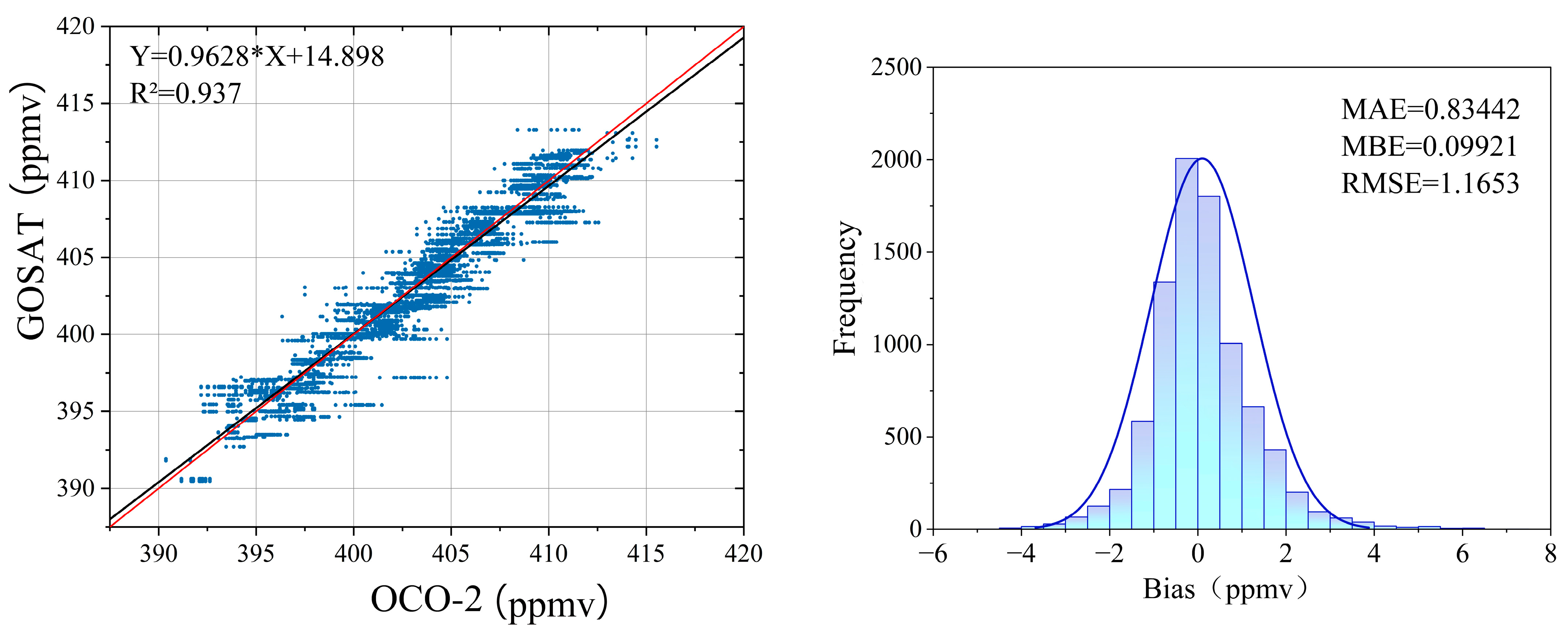
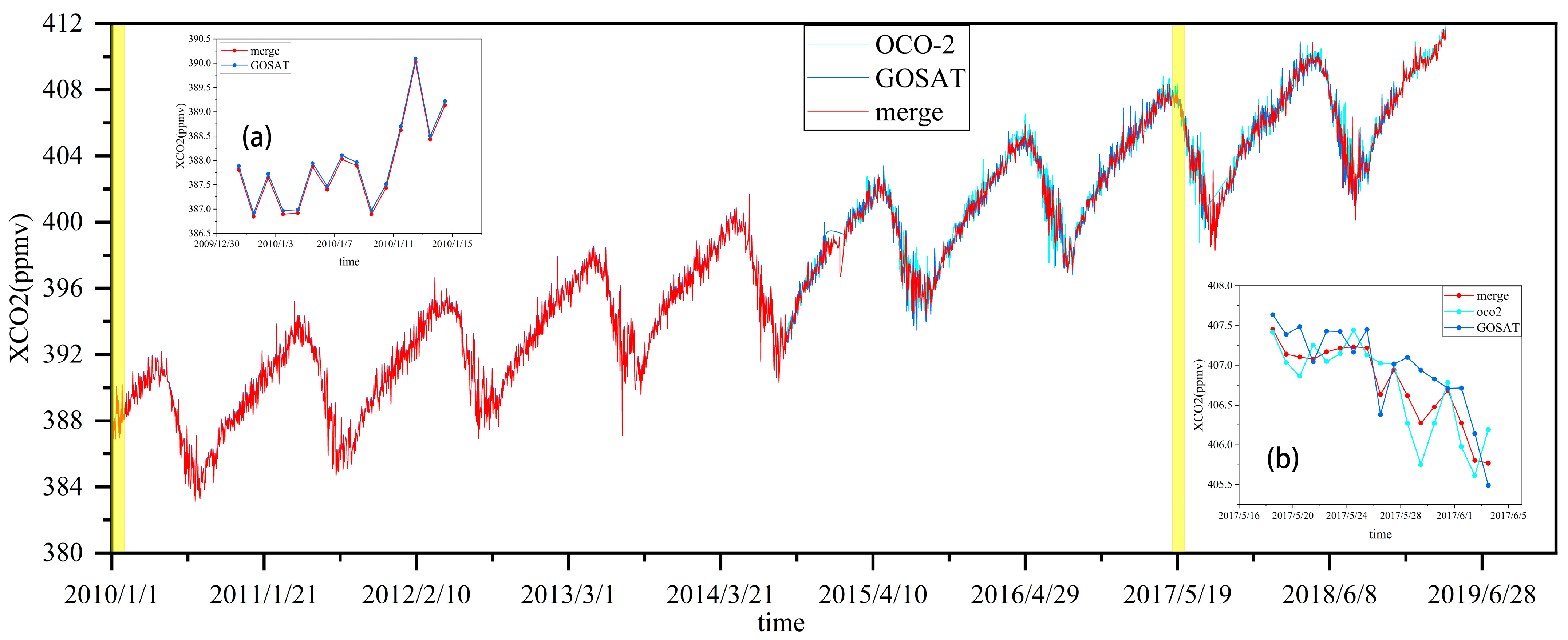
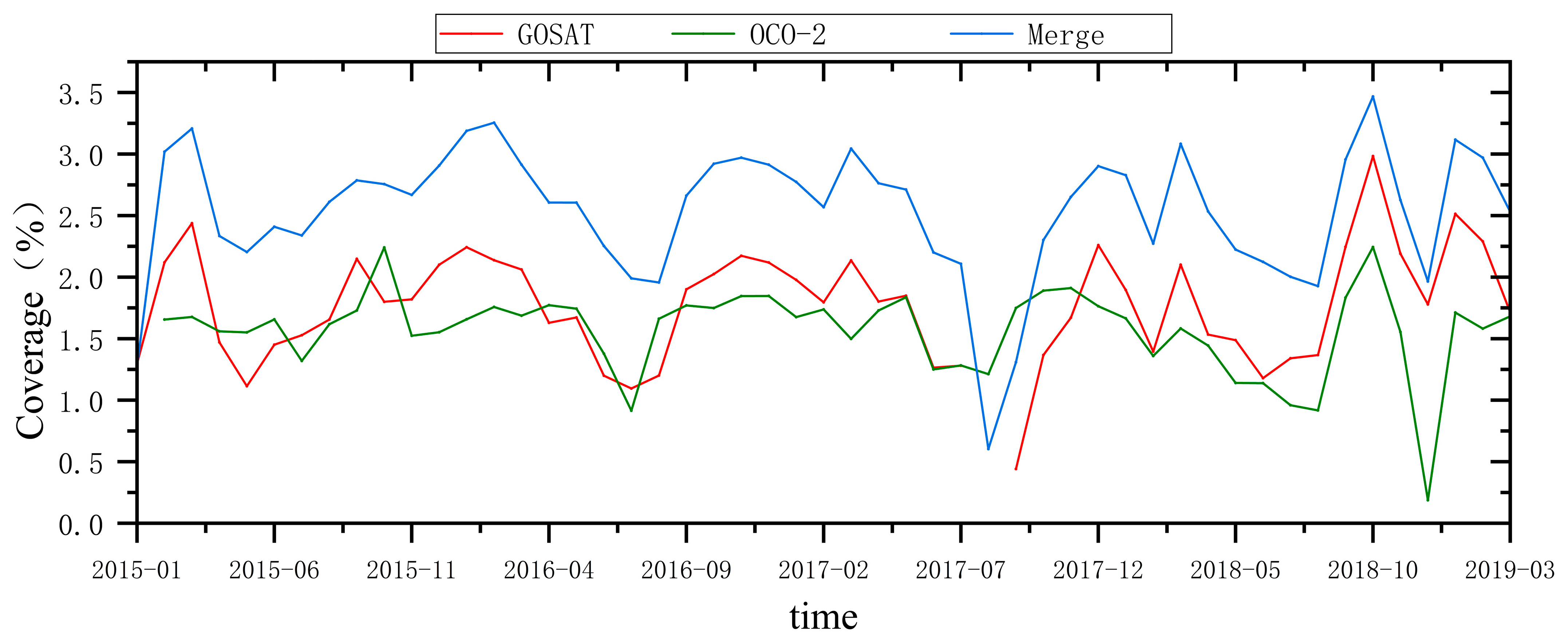
3.2. Grid Integration

This study extracted the average values of original data from two satellites (GOSAT and OCO-2) and the fused XCO₂ data within a 10 km radius around Hefei Station [119.17° E, 31.9° N]. Figure 7 presents a comparison between the original satellite data and the fused data. The single-satellite data (OCO-2 and GOSAT) show data gaps during certain periods, such as from May 2017 to June 2018, resulting in discontinuous records. In contrast, the fused data provides daily coverage from 1 January 2010, to 8 June 2019, achieving a complete time series and compensating for the temporal limitations of individual satellites.

Figure 8 shows the monthly spatial coverage of the three datasets from January 2015 to March 2019, with the spatial resolution of both the GOSAT and fusion datasets being 10 km, while the OCO-2 data has a higher resolution of 2.25 × 1.29 km. From the line chart, the spatial coverage of GOSAT and OCO-2 data is low, and fluctuates over time, showing a certain instability. Specifically, the average spatial coverage of GOSAT data was 1.44% and that of OCO-2 data was 1.54%, both of which failed to achieve a high level of coverage. However, under the effect of the grid integration method, the average spatial coverage of the fusion dataset is increased to 2.53%, which is about 64% higher than that of GOSAT and 64.3% higher than that of OCO-2. The results show that the spatial coverage of XCO2 remote sensing data in China can be effectively improved through data fusion, and provide more complete and high-quality observation data support for subsequent carbon source and sink research.

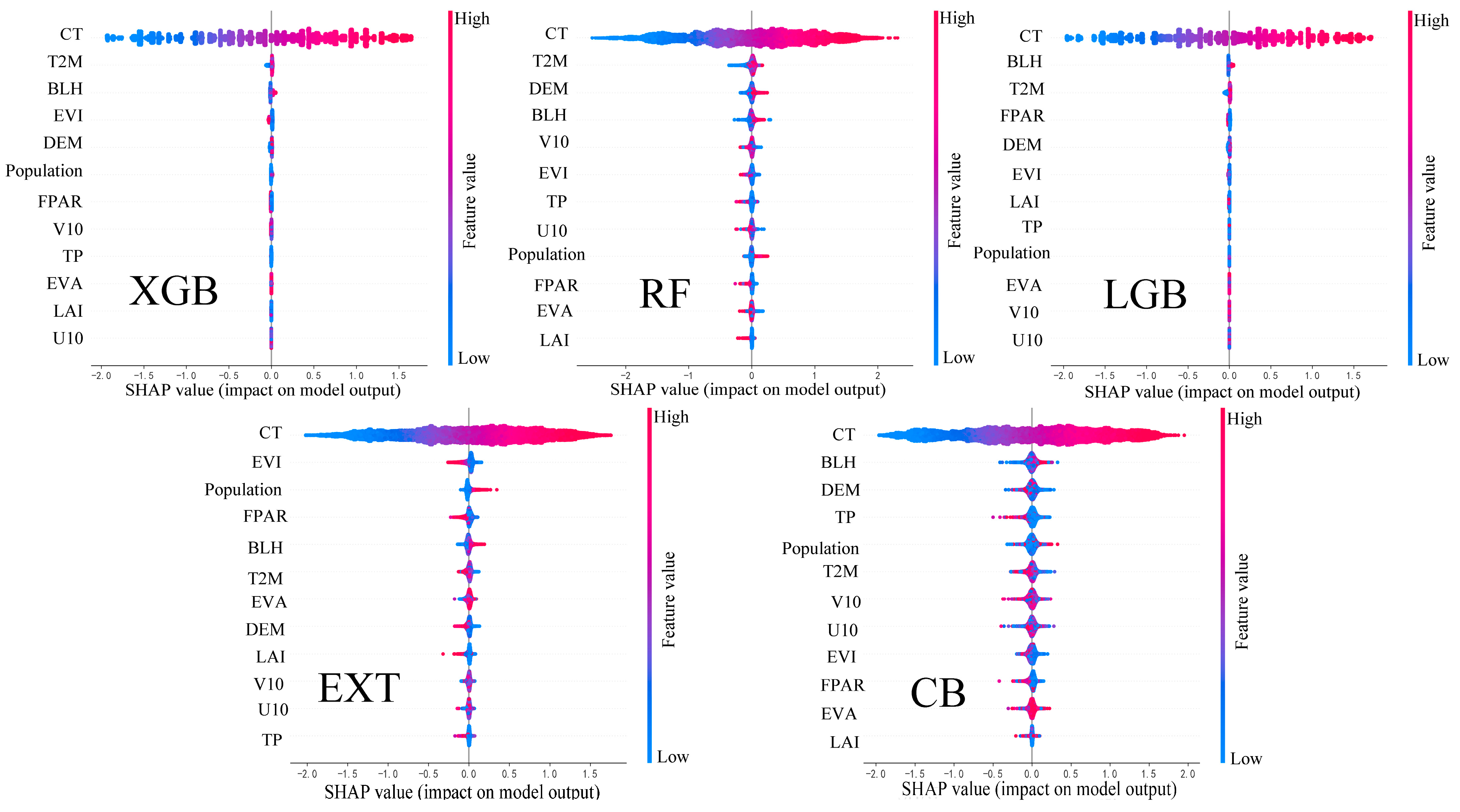
3.3. Variable Importance Estimation

Figure 9 presents the SHAP (Shapley Additive exPlanations) values for five machine learning models—XGB, RF, LGB, EXT, and CB. A higher SHAP value indicates a greater contribution of a feature to the model output. As shown in the figure, CT, representing the simulated CO₂ concentration data, consistently exhibits high average SHAP values ranging from 0.5 to 0.6 across all models. Other features, such as T2M and BLH, also demonstrate significant influence in most models.

The XGB model assigns relatively high importance to a few key features, notably T2M and BLH, with average SHAP values of approximately 0.35 and 0.3, respectively. The RF model distributes feature importance more evenly, suggesting a more balanced overall structure. The LGB model emphasizes a small number of dominant features, particularly BLH and T2M, with average SHAP values of 0.7 and 0.25, respectively. The EXT model, characterized by higher randomness, exhibits a broader distribution of feature importance, contributing to increased model diversity. The CB model, based on a symmetric tree structure, offers enhanced computational efficiency and stability.

Overall, the differences among these models result in complementary feature selection behaviors. When combined in a stacked ensemble, they can collectively capture a wider range of information relevant to CO₂ concentration, thereby improving the accuracy and robustness of the estimation.

3.4. Validation of the Reconstructed XCO₂

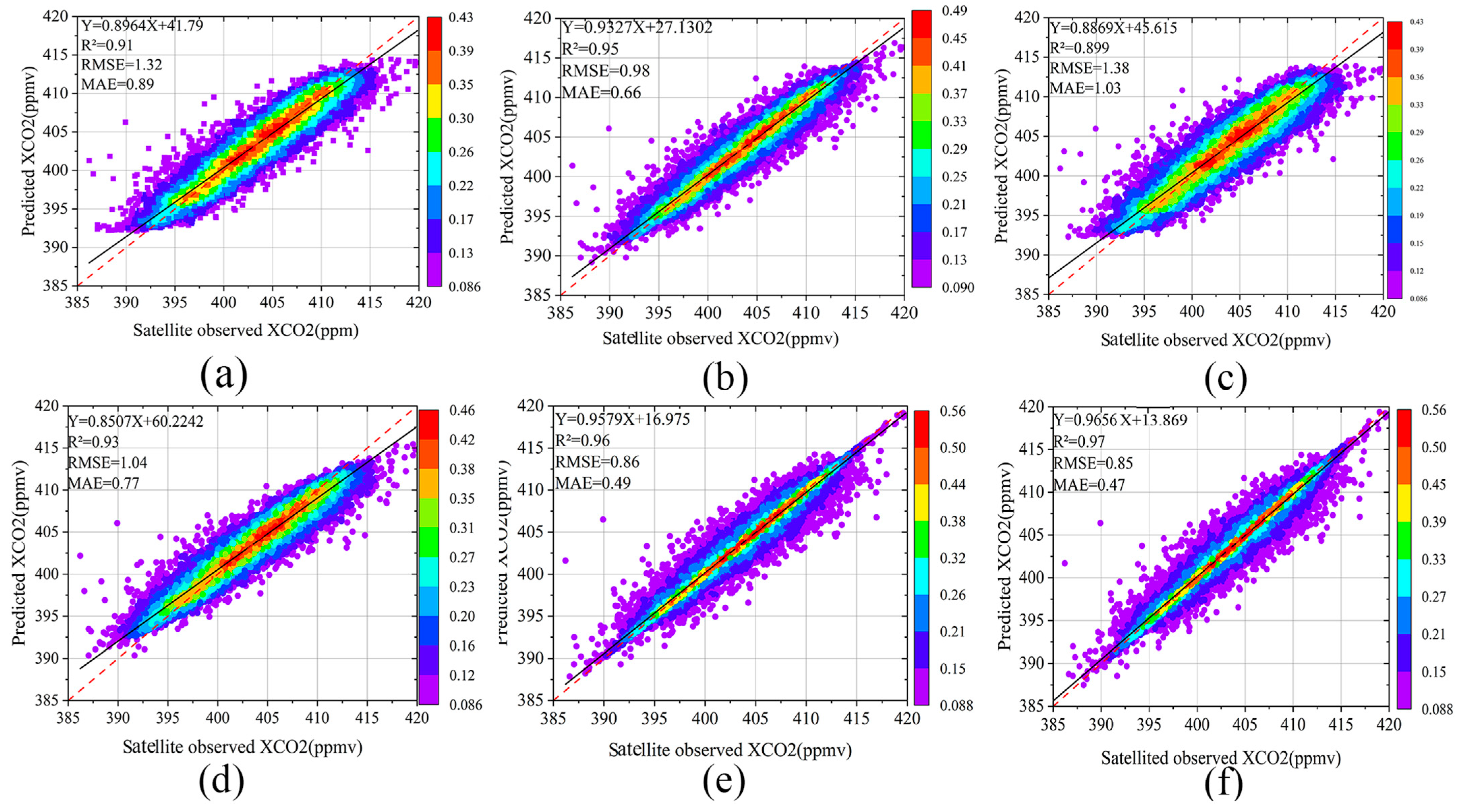
3.4.1. Performance Validation of the MLSM-XE Model

Figure 10a–e compare the ten-fold cross-validation results of five machine learning models: XGB, RF, LGB, EXT, and CB. Their respective R² values are 0.91, 0.95, 0.89, 0.93, and 0.95, with corresponding RMSEs of 1.32, 0.98, 1.38, 1.04, and 0.86 ppmv, and MAEs of 0.89, 0.66, 1.03, 0.77, and 0.49 ppmv. Among these, the CB and RF models demonstrated higher accuracy in estimating XCO₂ concentrations, while the LGB model performed the worst.

All five models exhibited a tendency to overestimate XCO₂ concentrations when values were below 405 ppmv (as indicated by the red dashed line appearing below the black solid line in Figure 8), and to underestimate them when concentrations exceeded 405 ppmv. The CB model achieved the highest R² value (0.95) and also yielded the lowest RMSE and MAE among the five models, at 0.86 ppmv and 0.49 ppmv, respectively.

Figure 10f shows the ten-fold cross-validation result of the MLSM-XE model, which achieved an R² of 0.97, higher than any of the five individual models. Its RMSE and MAE were 0.85 ppmv and 0.47 ppmv, respectively, both lower than those of the single models. Although the MLSM-XE model also showed overestimation when XCO₂ concentrations were below 410 ppmv and underestimation above 410 ppmv, its overall fit was closest to the standard trend line. Compared to the individual machine learning models, the MLSM-XE model produced more centralized estimates and demonstrated the best overall performance.

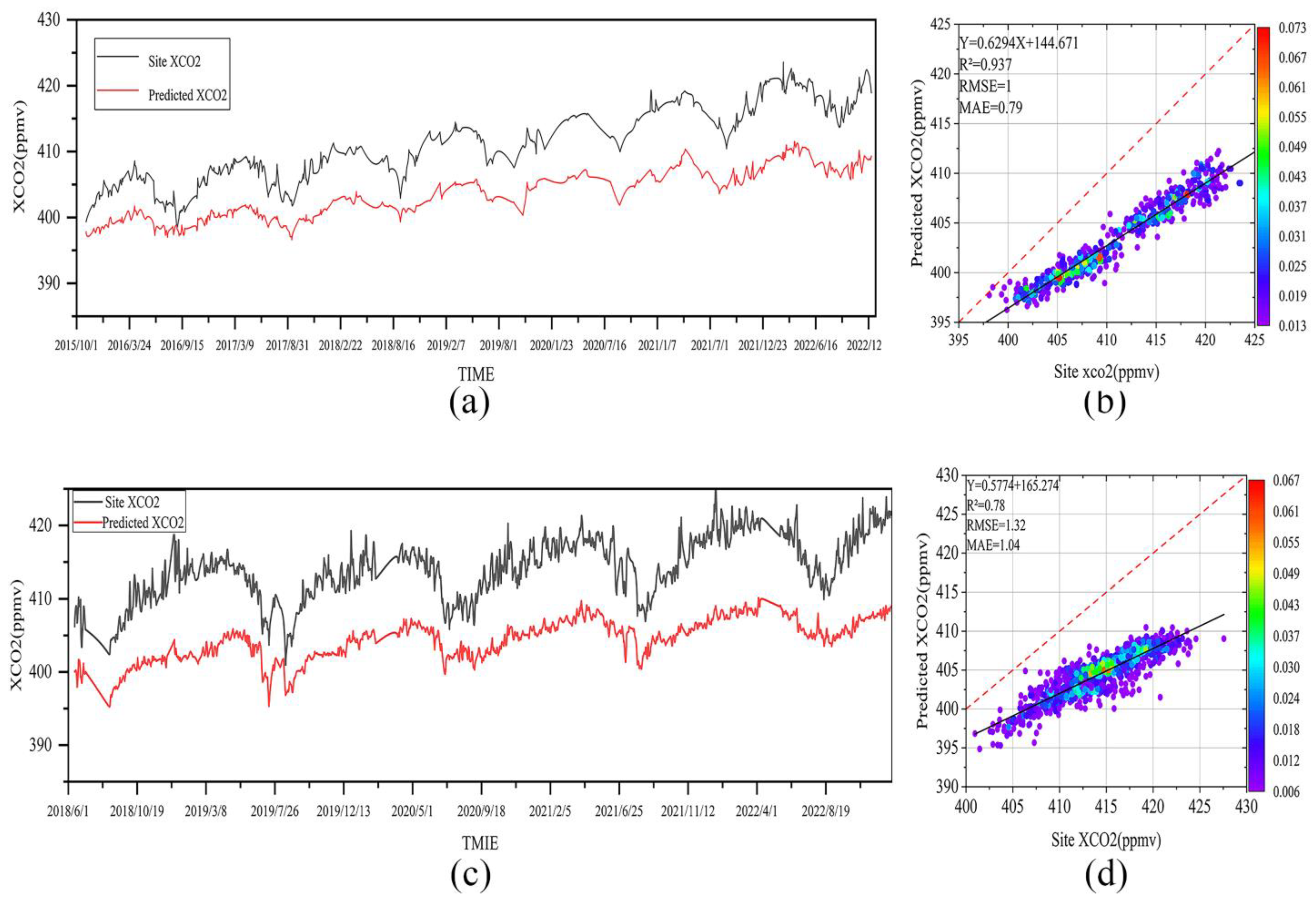
3.4.2. Validation with Ground-Based Monitoring Stations

Figure 11 presents the comparison results between two ground stations and the model-estimated XCO₂ concentrations. From Figure 11b,d, it is evident that the most accurate results were observed at Hefei Station, where the highest R² (0.93), lowest RMSE (1 ppmv), and lowest MAE (0.79 ppmv) were achieved within grid cells of less than 1 km. In contrast, Xianghe Station performed relatively poorly, with an R² of 0.78, and corresponding RMSE and MAE values of 1.32 ppmv and 1.04 ppmv, respectively.

As shown in Figure 11a,c, the temporal variation trend of the model-estimated XCO₂ concentration closely aligns with the time series of the XCO₂ concentrations observed at the stations. It can also be seen that the model-estimated XCO₂ concentrations were generally lower than the station-observed concentrations. The main reason for this discrepancy is that the station-based measurements directly capture CO₂ concentrations near the surface using fixed ground instruments, which typically focus on concentrations close to the ground. In contrast, satellite observations, which rely on remote sensing technology, capture XCO₂ values that reflect the distribution of CO₂ at various heights within a given area, rather than just near-surface concentrations. The general underestimation of satellite-observed XCO₂ compared to ground station measurements is attributed to the higher CO₂ concentrations near the surface due to local emission sources and plant respiration. As altitude increases, the gas is diluted, and while convective flows and turbulence in the lower atmosphere help mix gases, there is less effective mixing at higher altitudes, away from surface sources, leading to relatively lower CO₂ concentrations [29].

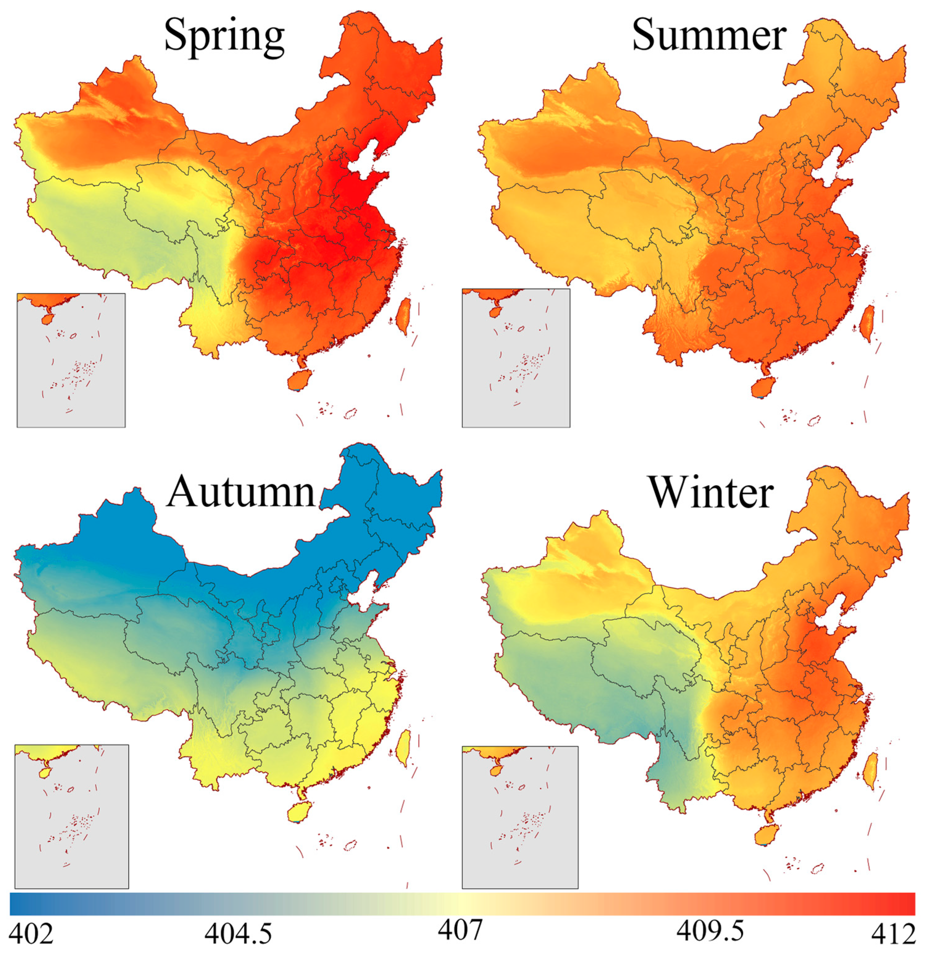
3.5. Spatial Distribution of CO₂ in China

Figure 12 presents the quarterly average variation in XCO₂ concentrations across China from 2010 to 2022, highlighting significant seasonal differences in XCO₂ concentrations and their spatial distribution patterns. As observed in the figure, the highest average XCO₂ concentration occurred in the spring (410.35 ppmv), with concentrations fluctuating between 406.90 ppmv and 412.04 ppmv across various provinces. During spring, the XCO₂ concentration in the North China Plain reached 410.44 ppmv. Eastern China, including the Sichuan Basin, Weihe Plain, and regions in the southeast and northeast, also showed relatively high XCO₂ concentrations at this time. In contrast to spring, the summer months had the lowest average XCO₂ concentration (404.63 ppmv). Regions such as the Qinghai–Tibet Plateau and South China exhibited higher XCO₂ concentrations, with some areas exceeding 404.33 ppmv. The northeastern region showed the lowest concentrations, typically below 403.76 ppmv. In autumn, the XCO₂ concentration slightly increased, with an average value of 405.33 ppmv. The highest XCO₂ concentrations were observed in the boundaries of Shandong, Hebei, and neighboring provinces, such as Henan, Anhui, and Hubei, with values around 407 ppmv. During winter, XCO₂ concentrations significantly increased, reaching an average of 409.27 ppmv. The XCO₂ concentrations in the North China Plain and the lower reaches of the Yangtze River approached the spring peak value.

It is noteworthy that the seasonal pattern of XCO₂ concentrations exhibited regional differences across China. While the peak XCO₂ concentrations typically occurred in spring, the lowest concentrations showed significant geographic variation. For instance, in regions such as the Qinghai–Tibet Plateau, Guangxi, Guangdong, Hong Kong–Macau–Taiwan, and southern provinces like Jiangxi, Hunan, and Guizhou, the lowest XCO₂ concentrations were observed in autumn. In contrast, northern China often experiences lower XCO₂ concentrations during summer, which may be linked to the region’s rich black soil resources. Black soil has a strong carbon sink capacity, promoting plant photosynthesis [16] and effectively storing CO₂ [30], further reducing atmospheric CO₂ concentrations.

3.6. Long-Term Variation Characteristics of CO₂ Concentrations in China

Figure 13 presents the annual average changes in XCO₂ concentrations in China from 2010 to 2022, reflecting the long-term trend of XCO₂ levels in the country. The data show that the national annual average XCO₂ concentration increased from 403.149 ppmv in 2010 to 410.656 ppmv in 2022, exhibiting an overall upward trend. However, this change was not uniform, with significant fluctuations observed between 2013 and 2014. In 2013, the XCO₂ concentration reached 409.081 ppmv, nearly matching the level observed in 2022. This spike was largely due to the most severe haze weather in 52 years, which occurred in 2013 [31]. Haze weather is typically caused by high energy consumption and pollutant emissions, which directly contribute to increases in CO₂. At the same time, the suppression of plant photosynthesis further reduced CO₂ absorption, leading to a significant rise in atmospheric CO₂ concentrations. Therefore, the occurrence of haze in 2013 not only represents the direct impact of extreme weather events on air quality but also highlights the complex relationship between CO₂ concentration fluctuations and environmental pollution [32].

In contrast to 2013, the XCO₂ concentration decreased to 405.08 ppmv in 2014, indicating that, despite the high CO₂ accumulation in 2013, environmental factors and policy adjustments played a corrective role in the following period. Between 2017 and 2018, China’s XCO₂ concentration showed a downward trend, which can be attributed to a series of environmental protection and resource conservation policies implemented by the Chinese government starting in 2017 [33]. After the 19th National Congress of the Communist Party, China vigorously promoted the development and application of renewable energy, encouraging enterprises and individuals to invest in clean energy projects, such as solar and wind power. Compared to traditional fossil fuels, the use of these clean energy sources significantly reduced CO₂ emissions. Therefore, the reduction in CO₂ concentrations between 2017 and 2018 was not only a result of economic structural transformation and energy policy adjustments but also a response to national efforts to address climate change.

Although CO₂ concentrations in China are still on the rise, the effective intervention of policies has notably slowed this increase, laying a solid foundation for balancing economic development and environmental protection in the future. With the continued advancement of these policies and the collective efforts from all sectors of society, China is expected to achieve even greater success in addressing climate change and promoting sustainable development.

3.7. Discussion

In this study, by integrating data from two carbon-monitoring satellites and employing a multi-model ensemble machine learning approach, a high-precision XCO₂ concentration estimation model for China was successfully developed. The application of data fusion techniques significantly improved both the spatiotemporal resolution and prediction accuracy of the model, effectively addressing challenges related to spatiotemporal consistency and uncertainties in multi-source remote sensing data. The integration of observations from both satellites helped fill the spatial and temporal gaps present in single-satellite data, optimizing the quality of the training dataset. This fusion not only enhanced model accuracy but also reduced the impact of missing data and observational errors, enabling a more comprehensive capture of the spatial heterogeneity and dynamic trends of carbon emissions.

In terms of data processing, systematic adjustments and standardization were applied to account for differences in sensor sensitivity, spatiotemporal resolution, observation timing, and retrieval priors between the satellite datasets. As a result, a temporally consistent, standardized long-term XCO₂ dataset was generated, overcoming limitations in temporal continuity associated with single-satellite observations. Compared to studies relying on single satellite data (Guo et al., 2012; He et al., 2022; He et al., 2023) [34,35,36], this research achieved broader temporal coverage and higher data density by fusing multi-source satellite data, enhancing the model’s ability to capture long-term variation trends. This provides reliable analytical support for addressing complex seasonal fluctuations and climate change processes.

On the modeling side, this study adopted a stacked ensemble method using linear regression as the meta-learner, effectively integrating the prediction results of five base learners: LGB, XGB, CB, RF, and EXT. The ensemble model improved accuracy by 0.6 percentage points compared to the standalone LGB model. LGB and XGB dominated in modeling high-dimensional nonlinear features, CB enhanced the model’s robustness to noisy data, while RF and EXT contributed to global stability and robustness. Through dynamic weight allocation, the linear regression meta-learner effectively mitigated overfitting issues of individual models, compensated for the limitations in low-dimensional modeling, and improved the model’s capability to capture local patterns. Overall, the ensemble learning algorithm significantly enhanced the accuracy and precision of CO₂ concentration prediction [37,38,39].

This study provides critical data support for formulating regionally differentiated emission reduction policies, coordinated air pollution management, and public health early warning systems, while also offering a replicable technical framework for building carbon monitoring systems in developing countries. It not only facilitates the scientific implementation of China’s “dual carbon” goals but also makes significant data and methodological contributions to global climate change mitigation efforts. This innovative research demonstrates remarkable interdisciplinary value and societal significance across multiple dimensions, including environmental governance, public health, and global climate action.

4. Conclusions

This study integrates XCO₂ data from two carbon satellites and combines various auxiliary data that influence CO₂ concentrations. An ensemble learning model based on multiple machine learning models was developed to estimate XCO₂ concentrations across China from 2010 to 2022, with a resolution of up to 1 km. Model validation and ground-based verification demonstrate that the dataset has high accuracy. The main conclusions and contributions are as follows:

(1)

The XCO₂ product data from the GOSAT and OCO-2 satellites were successfully integrated, resulting in a more complete overall time series. This effectively reduced the spatiotemporal data gaps caused by the limited observations from a single satellite, enhancing the data coverage.

(2)

A machine learning ensemble model for estimating regional XCO₂ in China was successfully developed, achieving strong performance in sample-based cross-validation (R² = 0.97, RMSE = 0.85 ppmv) and ground validation (R² values of 0.93 and 0.78, with corresponding RMSEs of 1.00 ppmv and 1.32 ppmv).

(3)

The seasonal characteristics of XCO₂ concentrations in China were revealed: the highest concentrations typically occurred in the spring, followed by a decrease in summer to the lowest values, gradually rising with seasonal changes and reaching a peak again in the following spring. As for annual variation, the XCO₂ concentrations in China have been rising year by year, but air pollution control and energy-saving policies have slowed the upward trend of XCO₂. The fluctuations in XCO₂ concentrations from 2010 to 2022 reveal that China faces dual challenges of economic development and environmental protection in addressing climate change and carbon emission pressures. While rapid economic growth and urbanization have driven increasing energy demand, thereby exacerbating CO₂ emissions, environmental protection policies and sustainable development initiatives have effectively slowed the rate of XCO₂ concentration growth. Consequently, the annual variations in CO₂ concentrations are influenced not only by natural factors but also profoundly shaped by socioeconomic factors, such as policy adjustments and industrial transformation. With the maturation of clean energy technologies and strengthened policy guidance, China’s CO₂ concentrations are expected to trend toward a more stable and low-carbon trajectory.

References

1. AR5 Synthesis Report: Climate Change 2014—IPCC[EB/OL]. Available online: https://www.ipcc.ch/report/ar5/syr/ (accessed on 4 March 2025).
2. Wunch, D.W.P.O. A method for evaluating bias in global measurements of CO2 total columns from space. Atmos. Chem. Phys. Discuss. 2011, 11, 20899–20946. [Google Scholar] [CrossRef]
3. Yu, R.; Zhang, Y.; Wang, J.; Li, J.; Chen, H.; Gong, J.; Chen, J. Recent Progress in Numerical Atmospheric Modeling in China. Adv. Atmos. Sci. 2019, 36, 938–960. [Google Scholar] [CrossRef]
4. Nguyen, P.; Shivadekar, S.; Chukkapalli, S.S.L.; Halem, M. Satellite data fusion of multiple observed XCO2 using compressive sensing. In Proceedings of the Signal Processing, Sensor/Information Fusion, and Target Recognition XXIX, Online, 27 April–8 May 2020; Volume 11423, pp. 219–231. [Google Scholar]
5. Hu, K.; Liu, Z.; Shao, P.; Feng, X.; Zhang, Q.; Weng, L.; Wang, Y.; Di, L.; Xia, M. Study on high temporal and spatial resolution XCO2 concentration estimation based on carbon satellite data. Chin. J. Atmos. Sci. 2024, 47, 976–992. [Google Scholar]
6. Siabi, Z.; Falahatkar, S.; Alavi, S.J. Spatial distribution of XCO2 using OCO-2 data in growing seasons. J. Environ. Manag. 2019, 244, 110–118. [Google Scholar] [CrossRef]
7. Li, J.; Jia, K.; Wei, X.; Xia, M.; Chen, Z.; Yao, Y.; Zhang, X.; Jiang, H.; Yuan, B.; Tao, G.; et al. High-spatiotemporal resolution mapping of spatiotemporally continuous atmospheric CO2 concentrations over the global continent. Int. J. Appl. Earth Obs. Geoinf. 2022, 108, 102743. [Google Scholar] [CrossRef]
8. Girach, I.A.; Ponmalar, M.; Murugan, S.; Rahman, P.A.; Babu, S.S.; Ramachandran, R. Applicability of Machine Learning Model to Simulate Atmospheric CO2 Variability. IEEE Trans. Geosci. Remote Sens. 2022, 60, 4107306. [Google Scholar] [CrossRef]
9. Seamless Mapping of Long-Term (2010–2020) Daily Global XCO2 and XCH4 from the Greenhouse Gases Observing Satellite (GOSAT), Orbiting Carbon Observatory 2 (OCO-2), and CAMS Global Greenhouse Gas Reanalysis (CAMS-EGG4) with a Spatiotemporally Self-Supervised Fusion Method[EB/OL]. Available online: https://essd.copernicus.org/articles/15/3597/2023/ (accessed on 4 March 2025).
10. He, Q.; Ye, T.; Chen, X.; Dong, H.; Wang, W.; Liang, Y.; Li, Y. Full-coverage mapping high-resolution atmospheric CO2 concentrations in China from 2015 to 2020: Spatiotemporal variations and coupled trends with particulate pollution. J. Clean. Prod. 2023, 428, 139290. [Google Scholar] [CrossRef]
11. Zhang, M.; Liu, G. Mapping contiguous XCO2 by machine learning and analyzing the spatio-temporal variation in China from 2003 to 2019. Sci. Total Environ. 2023, 858, 159588. [Google Scholar] [CrossRef]
12. Zhang, Y. Study on Spatialization and Spatiotemporal Variation of Atmospheric XCO2 in China Based on Multi-Source Remote Sensing Data. Master’s Thesis, Nanjing University of Information Science and Technology, Nanjing, China, 2024. [Google Scholar]
13. Yokota, T.; Yoshida, Y.; Eguchi, N.; Ota, Y.; Tanaka, T.; Watanabe, H.; Maksyutov, S. Global Concentrations of CO2 and CH4 Retrieved from GOSAT: First Preliminary Results. SOLA 2009, 5, 160–163. [Google Scholar] [CrossRef]
14. Eldering, A.; O’Dell, C.W.; Wennberg, P.O.; Crisp, D.; Gunson, M.R.; Viatte, C.; Avis, C.; Braverman, A.; Castano, R.; Chang, A.; et al. The Orbiting Carbon Observatory-2: First 18 months of science data products. Atmos. Meas. Tech. 2017, 10, 549–563. [Google Scholar] [CrossRef]
15. Liang, A.; Gong, W.; Han, G.; Xiang, C. Comparison of Satellite-Observed XCO2 from GOSAT, OCO-2, and Ground-Based TCCON. Remote Sens. 2017, 9, 1033. [Google Scholar] [CrossRef]
16. Jacobs, N. Quality controls, bias, and seasonality of CO2 columns in the boreal forest with Orbiting Carbon Observatory-2, Total Carbon Column Observing Network, and EM27/SUN measurements. Atmos. Meas. Tech. 2020, 13, 5033–5063. [Google Scholar] [CrossRef]
17. Peters, W.; Jacobson, A.R.; Sweeney, C.; Andrews, A.E.; Conway, T.J.; Masarie, K.; Miller, J.B.; Bruhwiler, L.M.P.; Pétron, G.; Hirsch, A.I.; et al. An atmospheric perspective on North American carbon dioxide exchange: CarbonTracker. Proc. Natl. Acad. Sci. USA 2007, 104, 18925–18930. [Google Scholar] [CrossRef]
18. Wunch, D.; Toon, G.C.; Wennberg, P.O.; Wofsy, S.C.; Stephens, B.B.; Fischer, M.L.; Uchino, O.; Abshire, J.B.; Bernath, P.; Biraud, S.C.; et al. Calibration of the total carbon column observing network using aircraft profile data. Atmos. Meas. Tech. 2010, 3, 1351–1362. [Google Scholar] [CrossRef]
19. Büyükçakir, B.; Mutlu, A.Y. Comparison of Hilbert Vibration Decomposition with Empirical Mode Decomposition for Classifying Epileptic Seizures. In Proceedings of the 2018 52nd Asilomar Conference on Signals, Systems, and Computers, Pacific Grove, CA, USA, 28–31 October 2018. [Google Scholar]
20. Watanabe, H.; Hayashi, K.; Saeki, T.; Maksyutov, S.; Nasuno, I.; Shimono, Y.; Hirose, Y.; Takaichi, K.; Kanekon, S.; Ajiro, M.; et al. Global mapping of greenhouse gases retrieved from GOSAT Level 2 products by using a kriging method. Int. J. Remote Sens. 2015, 36, 1509–1528. [Google Scholar] [CrossRef]
21. Jeong, S.; Zhao, C.; Andrews, A.E.; Dlugokencky, E.J.; Sweeney, C.; Bianco, L.; Wilczak, J.M.; Fischer, M.L. Seasonal variations in N2O emissions from central California. Geophys. Res. Lett. 2012, 39, L16801–L16805. [Google Scholar] [CrossRef]
22. Sheng, M. Study on the Response of Atmospheric CO2 Concentration Changes Monitored by Multi-Source Carbon Satellite Remote Sensing to Anthropogenic Emissions. Ph.D. Thesis, University of Chinese Academy of Sciences, Beijing, China, 2022. [Google Scholar]
23. Rodgers, C.D.; Connor, B.J. Intercomparison of remote sounding instruments. J. Geophys. Res. Atmos. 2003, 108, 4116. [Google Scholar] [CrossRef]
24. LightGBM: A Highly Efficient Gradient Boosting Decision Tree|Semantic Scholar[EB/OL]. Available online: https://www.semanticscholar.org/paper/LightGBM%3A-A-Highly-Efficient-Gradient-Boosting-Tree-Ke-Meng/497e4b08279d69513e4d2313a7fd9a55dfb73273 (accessed on 5 March 2025).
25. XGBoost: A Scalable Tree Boosting System|Semantic Scholar[EB/OL]. Available online: https://www.semanticscholar.org/paper/XGBoost%3A-A-Scalable-Tree-Boosting-System-Chen-Guestrin/26bc9195c6343e4d7f434dd65b4ad67efe2be27a (accessed on 5 March 2025).
26. Dorogush, A.V.; Ershov, V.; Gulin, A. CatBoost: Gradient boosting with categorical features support. arXiv 2018, arXiv:1810.11363. [Google Scholar]
27. Breiman, L. Random Forests. Mach. Learn. 2001, 45, 5–32. [Google Scholar] [CrossRef]
28. Geurts, P.; Ernst, D.; Wehenkel, L. Extremely randomized trees. Mach. Learn. 2006, 63, 3–42. [Google Scholar] [CrossRef]
29. Houghton, R.A. Balancing the Global Carbon Budget. Annu. Rev. Earth Planet. Sci. 2007, 35, 313–347. [Google Scholar] [CrossRef]
30. Cui, Q.; Xia, J.; Yang, H.; Liu, J.; Shao, P. Biochar and effective microorganisms promote Sesbania cannabina growth and soil quality in the coastal saline-alkali soil of the Yellow River Delta, China. Sci. Total Environ. 2021, 756, 143801. [Google Scholar] [CrossRef] [PubMed]
31. China Meteorological News Press. China Greenhouse Gas Bulletin 2013. Chin. Environ. Sci. 2015, 35, 355. [Google Scholar]
32. Pu, S.; Zhang, X.; Chen, A.; Liu, Q.; Lian, X.; Wang, X.; Peng, S.; Wu, X. Impact of extreme climate events on carbon cycle of terrestrial ecosystems. Sci. China Earth Sci. 2019, 49, 1321–1334. [Google Scholar]
33. Chen, S.; Xi, C.; Ping, Z.; Chen, S.; Wang, X.; Luo, Q.; Cui, Z.; Huang, Y.; Wan, L.; Hou, X.; et al. Bioinformatics Analysis and Experimental Identification of Immune-Related Genes and Immune Cells in the Progression of Retinoblastoma. Investig. Ophthalmol. Vis. Sci. 2022, 63, 28. [Google Scholar] [CrossRef]
34. Guo, M.; Xu, J.; Wang, X.; He, H.; Li, J.; Wu, L. Estimating CO2 concentration during the growing season from MODIS and GOSAT in East Asia. Int. J. Remote Sens. 2015, 36, 4363–4383. [Google Scholar] [CrossRef]
35. He, S.; Dong, H.; Zhang, Z.; Yuan, Y. An Ensemble Model-Based Estimation of Nitrogen Dioxide in a Southeastern Coastal Region of China. Remote Sens. 2022, 14, 2807. [Google Scholar] [CrossRef]
36. He, Z.; Lei, L.; Zhang, Y.; Sheng, M.; Wu, C.; Li, L.; Zeng, Z.-C.; Welp, L.R. Spatio-Temporal Mapping of Multi-Satellite Observed Column Atmospheric CO2 Using Precision-Weighted Kriging Method. Remote Sens. 2020, 12, 576. [Google Scholar] [CrossRef]
37. Li, J.; Zhang, Y.; Gai, R. Estimation of CO2 column concentration in spaceborne shortwave infrared based on machine learning. Chin. Environ. Sci. 2023, 43, 1499–1509. [Google Scholar]
38. Liu, L.; Chen, L.; Liu, Y.; Yang, D.; Zhang, X.; Lu, N.; Ju, W.; Jiang, F.; Yin, Z.; Liu, G.; et al. Global Carbon Inventory Satellite Remote Sensing Monitoring Methods, Progress and Challenges. J. Remote Sens. 2022, 26, 243–267. [Google Scholar]
39. Wang, Z.; Sheng, M.; Xiao, W.; Yang, F.; Lin, B.; Xu, X.; Liu, Y. Spatial and temporal changes of XCO2 and anthropogenic CO2 emissions in China based on multi-source carbon satellite fusion products. Chin. Environ. Sci. 2023, 43, 1053–1063. [Google Scholar]
Figure 1. Relationship between prior XCO2 distribution and profile air pressure in each XCO2 product.
Atmosphere 16 00621 g001
Figure 2. Relationship between the column-averaged kernel function and profile pressure in various XCO2 products.
Atmosphere 16 00621 g002
Figure 3. Flow chart of MLSM-XE model construction.
Atmosphere 16 00621 g003
Figure 4. Time series plots of the difference between the original XCO2 values of the satellites and the adjusted XCO2 values.
Atmosphere 16 00621 g004
Figure 5. Correlation comparison between GOSAT and OCO-2 (before profile adjustment). The red line represents the X = Y reference line, while the black line indicates the fitted regression line.
Atmosphere 16 00621 g005
Figure 6. Correlation comparison between GOSAT and OCO-2 (after profile adjustment). The red line represents the X = Y reference line, while the black line indicates the fitted regression line.
Atmosphere 16 00621 g006
Figure 7. Line plot of XCO2 concentrations within a 10 km radius of the Hefei site with the original satellites (GOAST and OCO-2) and the fused satellite data. (a) Zoomed-in comparison chart from 30 December 2009 to 15 January 2010, and (b) magnified comparison chart from 16 May 2017 to 5 June 2017. The yellow bars indicate the corresponding regions for subplots (a,b) in the figure.
Atmosphere 16 00621 g007
Figure 8. The monthly spatial coverage of the three datasets from January 2015 to March 2019.
Atmosphere 16 00621 g008
Figure 9. SHAP values for each model factor.
Atmosphere 16 00621 g009
Figure 10. Scatter plots showing cross-validation of five machine learning and stacked models, with the red dotted line being the 1:1 fitting line And the black line represents the fitted regression line between observed values and predicted values. (a) The XGB model, (b) the RF model, (c) the LGB model, (d) the EXT model, (e) the CB model, and (f) the stacked model.
Atmosphere 16 00621 g010
Figure 11. Verification charts of predicted XCO2 and observed CO2 concentrations at ground stations. The red dashed line represents the X = Y reference line, while the solid black line indicates the fitted regression line between station observations and model predictions. (a) Line chart of Hefei Station from 2 November 2015 to 19 December 2022, and (b) scatter plot of CO2 concentration and predicted XCO2 concentration at Hefei Station. (c) Line chart of Xiang He Station from 14 June 2018 to 31 December 2022, and (d) scatter plot of CO2 concentration and predicted XCO2 at Xiang He Station.
Atmosphere 16 00621 g011
Figure 12. Predicts quarterly average concentrations of XCO2.
Atmosphere 16 00621 g012
Figure 13. Predicted annual average concentration of XCO2.
Atmosphere 16 00621 g013