Relationships Among Atmospheric Suspended Particulates with Different Sizes: A Case Study of Chongqing City

Abstract

The current study predicts that there would be scaling relationships among atmospheric suspended particulate materials (PMs) with different diameters. Through sampling the particulate materials concentration over different types of land use in municipal areas in Chongqing, analyzing the respective data of the independent concentrations of particulate materials varying in sizes, and testing the predictions, it is found that: (1) there are generally a negative relationships between falling dust of large particulate size (diameter > 10 μm) and floating dust of small ones (diameter ≤ 10 μm); (2) there are positive correlations among the fine particulate materials varying in sizes of iPM10, iPM2.5, and iPM1; (3) there is a disproportionately increase between the particulate materials varying in sizes compared to the respective control; (4) there is a declining-and-rising tendency between the particulate materials reduction rate and the increase in particulate materials along a particulate-size-decline gradient. The results of this study may contribute to understanding the law of the interactions of particulate materials with different particle sizes in the atmosphere and lay a theoretical foundation for the elimination of the atmospheric suspended pollutants.

1. Introduction

Atmospheric suspended particulate material caused by the rapid urbanization is becoming an important aspect of environmental research, and thus PM pollution is viewed as a critical problem in the environments of a megacity in China. So far, observations have discovered that there are diverse attributes of PMs with different particulate sizes differing greatly in, e.g., chemical composition and spatial distribution [1,2,3,4,5], physical properties and morphological characteristics [6,7], disperse routes [8], contribution to the formation of haze, particulate sources and sinks [4] and the degrees of harm to human health [9,10]. Generally, the PMs have been divided into two categories based on the particulate size of total suspended particulate material (TSP) in the atmosphere, i.e., falling/drifting dust, according to the statement in ‘Environmental Air Quality Standard’ promulgated by the Environmental Protection Administration in 1996, China (GB3095−1996 [11]).The former refers to the PMs with particulates of larger diameter (>10 μm) in the atmosphere settling down faster due to their heavier weight, while the latter refers to smaller ones with a diameter < 10 μm floating up in the atmosphere all year round due to lighter ones.

Studies have shown that PMs always undergo various atmospheric chemical reactions [12,13] which are responsible for changes in PM composition [14,15]. Moreover, a number of experiments in the past two decades have proved that the morphology of PMs has fractal structures [16,17,18,19,20,21]. If the above holds true, it can be inferred that the amount of PMs with different sizes are interrelated or size-dependent regularly instead of independent, respectively. In fact, some relationships among PMs were observed previously. For example, it was found that 60% of TSP was composed of sub-sized PMs in atmosphere monitoring in a middle school [22,23], and that atmospheric pollutants with sulfate ions were severely inhibited by the hygroscopicity of sea salt particulates [24]. Anthropogenic pollutants such as SO₂, NOx, organic matter interact with sea salt particulates in the northwest Pacific Ocean [25]. The interactions of odor-VOCs-PM also found that the abundance of the VOCs odor increased as the size variation in PMs [26].

For all that, little has been known about the serial relations among TSP-PM10-PM2.5-PM1 to date. Furthermore, because isolating harmful gases and fine inhalable particulates from PMs in the air has always been a permanent scientific problem, it is helpful to understand the potential law of interactions between PM particles of different sizes so as to control atmospheric pollutants and establish the rational planning of urban layout, adopting key measures for air pollution prevention. Furthermore, particles of different sizes can have a significant impact on human health, causing millions of deaths each year. It can be seen from this that the governance and improvement of urban air quality have become the most urgent research topics at present.

Although prior studies have examined the harm of inhalable particulate matter (PM) to human health from a macroscopic perspective and highlighted strategies for urban air pollution control, there remains a paucity of micro-level research. For instance, little attention has been paid to distinguishing the activity levels of particles of varying sizes in the atmosphere or leveraging the interaction mechanisms among particles of different sizes to enhance urban air pollution management. These aspects are crucial for addressing current and future urban environmental challenges and represent gaps in the existing literature that this study aims to address through supplementation and refinement. In the current study, areas with typical different vegetation types, human disturbance habitats, and land use types were selected in Chongqing City, western China. PM concentrations in the atmosphere were measured across days and four seasons, and the independent PM concentrations with different sizes, including iTSP, iPM10, iPM2.5, and iPM1, were calculated, and the correlations between the iPMs were examined, and the found laws were discussed. The purpose of the study is to understand the trends of the correlations among iPMs with different particulate sizes, which may lay a theoretical foundation for controlling and reducing the PMs in a megacity.

With the ongoing progression of urbanization, urban air pollution has emerged as a critical obstacle to the sustainable development of cities. This study not only elucidates the synergistic relationships among particles of varying sizes from a theoretical standpoint but also offers practical insights for promoting the healthy and sustainable development of present and future cities.

2. Methods

2.1. Study Area

The study area is situated in Shapingba district in Chongqing, which is in the west of the main urban area and to the east of the Sichuan Basin. Its southeastern part is backed by Gele Mountain, and the east is directly facing the Jialing River. The terrain is composed of hills, platforms, and low mountains, which transit from natural mountains to plains along the Yangtze River. There is a Geleshan National Forest Park located in the middle of Shapingba, with a total area of 9302.7 hm² and an altitudinal span of 160−690 m. There are abundant vegetation resources, which have the characteristics of natural, less-disturbed urban forest and artificial plant community as well, and there are relatively more days of good air quality in this area than in the other districts of the main city. In addition, this area is also a scientific, educational, and cultural center of Chongqing city where human activities are frequent and intense, and the PM10 and PM2.5 still exceed the state standard.

2.2. The Sampling Methods

(1)

Sampling sites and quadrat setting

The Three-Gorges-Square-business-circle was set as the study center in the Shapingba district of Chongqing city in 2017, and 19 sampling sites were selected in 2017, distributed as shown in Figure 1. Next, a total of 36 quadrats with the open land without vegetation coverage and non-greenland nearby were selected as control sites for each quadrat sample, so most of the control sites were close to their adjacent roads or open squares without trees. Due to the land-use types leading to the differences in the amount of dusting [27], the arrangement of sampling quadrats took account of factors such as the distances from the source of pollution, the elevation of the plant community, disturbances by humans, and the vegetation type and their tree species composition as well.

(2)

The sampling method for plant community and the arrangement of monitoring points

The quadrats for community were divided into two types, one of which was a square and the other a rectangle. First, the square was 20 m × 20 m in size. In order to detect the concentration of PMs both inside and outside the quadrat, five monitoring points were set up per quadrat, as shown in Figure 2I. Therein, A and B are the end points of the diagonal line, C and D are respectively at the 1/4 length from the end of the other diagonal line of the quadrat, E was the intersection of the two diagonal lines, and A, B, C, D, and E were set as monitoring points of a square quadrat. Second, the rectangular quadrat is 10 m × 20 m and 5 m × 20 m, as shown in Figure 2II,III. In order to measure the concentration of air particulate matter in the edge and interior of the former (Figure 2II), five monitoring points were also set up, wherein D and E were the end points of a diagonal line, A and C were the respective 1/4 length from the end of the other diagonal line of the quadrat, B was the intersection of the diagonal line, and A, B, C, D, and E were the monitoring points of a rectangle quadrat. In the latter one of the 5 m × 20 m rectangle quadrats (Figure 2III), five bisector points were taken as monitoring points of the sample in the midpoint connection line along the wide side of the rectangle quadrat.

2.3. Measurements for PMs Concentration

A hand-held DUSTMATE dust detector (resolution 0.1 μg/m³ with a range of 0–6000 μg/m³, rate 600 cc/min) was used to measure the four kinds of PMs concentrations, including TSP, PM10, PM2.5, and PM1, in different types of land in the study area. The experimenters were divided into two groups. The first group was monitored for 5 min at a 1.5 m high position above the ground, parallel to the human eye at each monitoring point, so as to collect the averaged data (μg/m³) at the interval of the period. Meanwhile, the meteorological factors, such as temperature, humidity, and wind speed, were also recorded using a Kestrel hand-held anemometer, and altitude and latitude positioning were recorded using UniStrong hand-held GPS and an iPhone compass. And the community’s canopy density and coverage were documented according to conventional field plant community survey methods. Meanwhile, another group of experimenters monitored the PMs concentration in the central area of the control point. The measurements per quadrat were finished within 40 min. All measurement points complete data collection at the same time to avoid errors caused by different time periods in the measurement data.

The measured parameter file of PMs concentration includes (1) diurnal variations in PMs: we chose to monitor PMs on sunny days after rainy days in August and December 2017 in order to avoid strong wind, heavy rain, frost, snow, fog, and haze on 5 August 2017 and 21 December 2017, due to PM concentration being closely related to those meteorological factors. The monitoring time point lasted for 12 h, from 7 a.m. to 7 p.m. hourly in the daytime, when temperature, humidity, and wind speed were recorded at the same time. (2) Seasonal variations in PMs concentration: the PMs were monitored for 12 months in the four seasons, including spring, summer, autumn, and winter. The measurements lasted three times a day at morning, midday, and night; three days in the first ten days, the middle ten days, and the last ten days of a month, which were three times a season in total. So the PMs concentration of each quadrat was monitored for nine days at a sampling site.

2.4. Land Use Types

There were forest lands in the study area, which “forest land” referred to the land covered by natural, secondary, or artificial forest. They were divided into five vegetation types, three disturbed plant communities, and five green space types. A vegetation type was the aggregation of plant communities based on the uniformity of life forms (primary or secondary), the same or similar edificator species, and the requirements for water and heat conditions. The five different vegetation types included evergreen broad-leaved forest, mixed forest, coniferous forest, deciduous broad-leaved forest, and sparse forest lawn (

Table A1. The average concentration of atmospheric suspended particulate matter in Shapingba District of Chongqing City. ± is the standard deviation of data. Among them, iTSP, iPM10, iPM2.5, and iPM1 are independent concentrations of PMs, and RR is reduction rate. Sp, S, F, and W refer to four seasons: spring, summer, autumn, and winter, respectively. FL = forest land, UBL = urban built-up land, GL = green land.

Season	Land Type	Site Category	iTSP (μg/m3)	ciTSP (μg/m3)	iTSP RR (%)	iPM10 (μg/m3)	ciPM10 (μg/m3)	iPM10 RR (%)	iPM2.5 (μg/m3)	ciPM2.5 (μg/m3)	iPM2.5 RR (%)	iPM1 (μg/m3)	ciPM1 (μg/m3)	iPM1 RR (%)
F	semi-natural	FL	49.00 ± 12.36	44.00 ± 15.24	0.11 ± 0.59	27.35 ± 10.87	39.28 ± 15.21	−0.30 ± 0.39	22.52 ± 6.85	32.27 ± 13.28	−0.30 ± 0.26	26.63 ± 8.33	27.15 ± 10.25	−0.02 ± 0.32
S	semi-natural	FL	37.40 ± 7.29	61.00 ± 10.35	−0.39 ± 0.23	15.80 ± 5.64	18.57 ± 8.64	−0.15 ± 0.15	17.74 ± 4.62	21.58 ± 8.33	−0.18 ± 0.12	10.36 ± 5.96	11.15 ± 6.12	−0.07 ± 0.21
Sp	semi-natural	FL	57.60 ± 10.21	65.30 ± 12.99	−0.12 ± 0.43	28.92 ± 9.23	24.75 ± 10.33	0.17 ± 0.32	27.68 ± 8.31	36.56 ± 11.64	−0.24 ± 0.23	24.6 ± 6.34	25.89 ± 8.47	−0.05 ± 0.43
W	semi-natural	FL	33.90 ± 15.29	41.10 ± 19.32	−0.18 ± 0.73	54.68 ± 13.5	64.51 ± 17.33	−0.15 ± 0.51	48.15 ± 14.69	46.77 ± 17.25	0.03 ± 0.42	35.47 ± 13.70	36.12 ± 11.98	−0.02 ± 0.57
F	broad-leaved evergreens	FL	29.20 ± 11.68	54.50 ± 21.8	−0.46 ± 0.49	26.34 ± 9.25	25.75 ± 8.50	0.02 ± 0.33	22.74 ± 6.08	35.30 ± 12.33	−0.36 ± 0.21	27.12 ± 9.01	27.15 ± 10.25	0.00 ± 0.29
S	broad-leaved evergreens	FL	30.10 ± 9.03	61.00 ± 27.45	−0.51 ± 0.26	12.89 ± 4.89	18.57 ± 7.43	−0.31 ± 0.12	17.55 ± 4.61	21.58 ± 7.69	−0.19 ± 0.16	11.36 ± 5.82	11.15 ± 6.12	0.02 ± 0.20
Sp	broad-leaved evergreens	FL	46.90 ± 16.41	57.80 ± 19.07	−0.19 ± 0.31	35.11 ± 12.33	42.38 ± 14.12	−0.17 ± 0.29	27.20 ± 8.06	30.43 ± 9.84	−0.11 ± 0.22	24.19 ± 6.03	25.89 ± 8.47	−0.07 ± 0.39
W	broad-leaved evergreens	FL	30.40 ± 14.59	51.10 ± 22.93	−0.41 ± 0.68	55.07 ± 15.21	64.51 ± 21.29	−0.15 ± 0.48	46.90 ± 13.78	46.77 ± 16.92	0.00 ± 0.45	36.33 ± 13.87	36.12 ± 11.98	0.01 ± 0.52
F	road	UBL	47.20 ± 16.14	44.00 ± 13.2	0.07 ± 0.37	34.84 ± 12.19	42.28 ± 15.22	−0.18 ± 0.42	22.38 ± 6.49	29.27 ± 8.20	−0.24 ± 0.29	27.98 ± 7.75	27.15 ± 6.98	0.03 ± 0.33
S	road	UBL	39.40 ± 15.73	61.00 ± 24.4	−0.35 ± 0.56	20.41 ± 8.16	18.57 ± 7.43	0.10 ± 0.47	19.14 ± 7.66	21.58 ± 8.63	−0.11 ± 0.45	11.25 ± 5.84	11.15 ± 5.96	0.01 ± 0.12
Sp	road	UBL	55.50 ± 13.87	65.30 ± 16.33	−0.15 ± 0.12	31.14 ± 7.79	24.75 ± 6.19	0.26 ± 0.14	31.84 ± 7.96	36.56 ± 9.14	−0.13 ± 0.09	24.32 ± 6.91	25.89 ± 7.26	−0.06 ± 0.31
W	road	UBL	34.60 ± 13.84	41.10 ± 13.44	−0.16 ± 0.42	62.17 ± 18.65	64.51 ± 22.58	−0.04 ± 0.25	49.26 ± 16.85	46.77 ± 15.43	0.05 ± 0.27	35.47 ± 12.08	36.12 ± 12.46	−0.02 ± 0.27
F	industry	UBL	43.70 ± 15.98	44.00 ± 13.2	−0.01 ± 0.36	36.21 ± 11.98	42.28 ± 15.22	−0.14 ± 0.39	20.03 ± 5.98	29.27 ± 8.20	−0.32 ± 0.27	30.16 ± 7.05	27.15 ± 6.98	0.11 ± 0.29
S	industry	UBL	34.60 ± 13.56	61.00 ± 24.4	−0.43 ± 0.55	20.49 ± 8.15	18.57 ± 7.43	0.10 ± 0.42	20.67 ± 8.72	21.58 ± 8.63	−0.04 ± 0.45	10.54 ± 4.98	11.15 ± 5.96	−0.05 ± 0.34
Sp	industry	UBL	51.50 ± 11.87	65.30 ± 16.33	−0.21 ± 0.23	30.84 ± 7.01	24.75 ± 6.19	0.25 ± 0.11	34.04 ± 9.10	36.56 ± 9.14	−0.07 ± 0.19	24.32 ± 7.03	25.89 ± 7.26	−0.06 ± 0.21
W	industry	UBL	31.00 ± 12.43	41.10 ± 13.44	−0.25 ± 0.46	63.51 ± 17.55	64.51 ± 22.58	−0.02 ± 0.24	46.83 ± 14.96	46.77 ± 15.43	0.00 ± 0.39	37.96 ± 12.64	36.12 ± 12.46	0.05 ± 0.33
F	public utilities	UBL	45.00 ± 15.31	44.00 ± 13.2	0.02 ± 0.29	26.01 ± 7.65	42.28 ± 15.22	−0.38 ± 0.33	24.17 ± 6.87	29.27 ± 8.20	−0.17 ± 0.23	26.12 ± 6.59	27.15 ± 6.98	−0.04 ± 0.19
S	public utilities	UBL	31.30 ± 12.46	61.00 ± 24.4	−0.49 ± 0.51	16.93 ± 5.59	18.57 ± 7.43	−0.09 ± 0.46	18.96 ± 9.16	21.58 ± 8.63	−0.12 ± 0.37	10.71 ± 5.01	11.15 ± 5.96	−0.04 ± 0.34
Sp	public utilities	UBL	43.70 ± 9.87	65.30 ± 16.33	−0.33 ± 0.31	30.75 ± 7.54	24.75 ± 6.19	0.24 ± 0.12	29.34 ± 6.19	36.56 ± 9.14	−0.20 ± 0.12	24.61 ± 7.34	25.89 ± 7.26	−0.05 ± 0.21
W	public utilities	UBL	25.30 ± 10.09	41.10 ± 13.44	−0.38 ± 0.42	60.39 ± 16.73	64.51 ± 22.58	−0.06 ± 0.24	46.45 ± 13.96	46.77 ± 15.43	−0.01 ± 0.36	35.76 ± 11.96	36.12 ± 12.46	−0.01 ± 0.31
F	garden	GL	47.70 ± 15.91	44.00 ± 13.2	0.08 ± 0.32	25.96 ± 7.05	42.28 ± 15.22	−0.39 ± 0.31	20.52 ± 5.47	29.27 ± 8.20	−0.30 ± 0.21	25.42 ± 7.01	27.15 ± 6.98	−0.06 ± 0.24
S	garden	GL	34.50 ± 11.43	61.00 ± 24.4	−0.43 ± 0.49	18.63 ± 6.63	18.57 ± 7.43	0.00 ± 0.48	14.01 ± 8.65	21.58 ± 8.63	−0.35 ± 0.35	9.56 ± 5.47	11.15 ± 5.96	−0.14 ± 0.38
Sp	garden	GL	44.00 ± 9.12	65.30 ± 16.33	−0.33 ± 0.11	33.14 ± 7.54	24.75 ± 6.19	0.34 ± 0.13	24.09 ± 5.46	36.56 ± 9.14	−0.34 ± 0.09	24.17 ± 7.68	25.89 ± 7.26	−0.07 ± 0.12
W	garden	GL	32.50 ± 7.21	41.10 ± 13.44	−0.21 ± 0.27	53.25 ± 14.21	64.51 ± 22.58	−0.17 ± 0.27	44.36 ± 14.12	46.77 ± 15.43	−0.05 ± 0.29	35.09 ± 10.96	36.12 ± 12.46	−0.03 ± 0.28
F	cornifer-broad mixed	FL	28.70 ± 12.65	54.50 ± 21.8	−0.47 ± 0.51	29.31 ± 11.06	25.75 ± 8.50	0.14 ± 0.41	23.07 ± 7.87	35.30 ± 12.33	−0.35 ± 0.19	26.12 ± 8.65	27.15 ± 10.25	−0.04 ± 0.29
S	cornifer-broad mixed	FL	35.30 ± 11.25	61.00 ± 27.45	−0.42 ± 0.29	10.08 ± 4.09	18.57 ± 7.43	−0.46 ± 0.21	16.41 ± 4.03	21.58 ± 7.69	−0.24 ± 0.15	10.71 ± 4.12	11.15 ± 6.12	−0.04 ± 0.31
Sp	cornifer-broad mixed	FL	50.20 ± 18.43	57.80 ± 19.07	−0.13 ± 0.64	34.82 ± 11.31	42.38 ± 14.12	−0.18 ± 0.32	26.17 ± 7.59	30.43 ± 9.84	−0.14 ± 0.23	24.61 ± 7.88	25.89 ± 8.47	−0.05 ± 0.42
W	cornifer-broad mixed	FL	30.90 ± 14.98	51.10 ± 22.93	−0.40 ± 0.45	60.44 ± 18.36	64.51 ± 21.29	−0.06 ± 0.18	46.40 ± 14.56	46.77 ± 16.92	−0.01 ± 0.42	35.76 ± 13.29	36.12 ± 11.98	−0.01 ± 0.50
F	residential	UBL	49.50 ± 16.11	44.00 ± 13.2	0.13 ± 0.25	25.46 ± 7.34	42.28 ± 15.22	−0.40 ± 0.26	21.82 ± 8.65	29.27 ± 8.20	−0.25 ± 0.23	27.12 ± 7.19	27.15 ± 6.98	0.00 ± 0.22
S	residential	UBL	35.70 ± 11.21	61.00 ± 24.4	−0.41 ± 0.42	17.17 ± 6.98	18.57 ± 7.43	−0.08 ± 0.47	16.27 ± 6.34	21.58 ± 8.63	−0.25 ± 0.41	11.36 ± 5.76	11.15 ± 5.96	0.02 ± 0.39
Sp	residential	UBL	49.70 ± 10.78	65.30 ± 16.33	−0.24 ± 0.09	31.56 ± 7.08	24.75 ± 6.19	0.28 ± 0.11	27.35 ± 7.12	36.56 ± 9.14	−0.25 ± 0.13	24.19 ± 7.63	25.89 ± 7.26	−0.07 ± 0.21
W	residential	UBL	31.40 ± 8.15	41.10 ± 13.44	−0.24 ± 0.31	57.34 ± 15.21	64.51 ± 22.58	−0.11 ± 0.29	45.03 ± 12.96	46.77 ± 15.43	−0.04 ± 0.30	36.33 ± 12.65	36.12 ± 12.46	0.01 ± 0.34
F	deciduous forest	FL	43.80 ± 20.14	54.50 ± 21.8	−0.20 ± 0.33	25.18 ± 5.22	25.75 ± 8.50	−0.02 ± 0.33	22.14 ± 8.05	35.30 ± 12.33	−0.37 ± 0.23	27.98 ± 8.02	27.15 ± 10.25	0.03 ± 0.23
S	deciduous forest	FL	49.10 ± 15.21	61.00 ± 27.45	−0.20 ± 0.21	17.26 ± 6.32	18.57 ± 7.43	−0.07 ± 0.19	17.69 ± 5.43	21.58 ± 7.69	−0.18 ± 0.15	11.25 ± 5.36	11.15 ± 6.12	0.01 ± 0.36
Sp	deciduous forest	FL	65.50 ± 28.16	57.80 ± 19.07	0.13 ± 0.50	30.64 ± 12.08	42.38 ± 14.12	−0.28 ± 0.25	29.24 ± 8.97	30.43 ± 9.84	−0.04 ± 0.28	24.32 ± 8.01	25.89 ± 8.47	−0.06 ± 0.48
W	deciduous forest	FL	29.60 ± 12.75	51.10 ± 22.93	−0.42 ± 0.46	65.14 ± 19.36	64.51 ± 21.29	0.01 ± 0.45	49.09 ± 15.61	46.77 ± 16.92	0.05 ± 0.52	35.47 ± 12.94	36.12 ± 11.98	−0.02 ± 0.52
F	planted forest	FL	48.80 ± 19.52	44.00 ± 15.24	0.11 ± 0.97	25.69 ± 11.25	39.28 ± 15.21	−0.35 ± 0.32	26.52 ± 7.65	32.27 ± 13.28	−0.18 ± 0.33	27.09 ± 10.23	27.15 ± 10.25	0.00 ± 0.12
S	planted forest	FL	38.00 ± 12.54	61.00 ± 10.35	−0.38 ± 0.54	16.28 ± 4.15	18.57 ± 8.64	−0.12 ± 0.17	20.59 ± 5.12	21.58 ± 8.33	−0.05 ± 0.24	10.83 ± 6.12	11.15 ± 6.12	−0.03 ± 0.32
Sp	planted forest	FL	59.20 ± 19.54	65.30 ± 12.99	−0.09 ± 0.63	27.95 ± 7.63	24.75 ± 10.33	0.13 ± 0.29	32.57 ± 10.98	36.56 ± 11.64	−0.11 ± 0.36	23.08 ± 5.97	25.89 ± 8.47	−0.11 ± 0.64
W	planted forest	FL	35.00 ± 14.21	41.10 ± 19.32	−0.15 ± 0.81	57.99 ± 12.92	64.51 ± 17.33	−0.10 ± 0.57	50.51 ± 15.27	46.77 ± 17.25	0.08 ± 0.58	35.4 ± 12.43	36.12 ± 11.98	−0.02 ± 0.61
F	grassland with sparse trees	GL	37.50 ± 17.27	54.50 ± 21.8	−0.31 ± 0.38	30.70 ± 7.69	25.75 ± 8.50	0.19 ± 0.27	21.72 ± 7.98	35.30 ± 12.33	−0.38 ± 0.26	27.98 ± 8.06	27.15 ± 10.25	0.03 ± 0.29
S	grassland with sparse trees	GL	44.90 ± 19.23	61.00 ± 27.45	−0.26 ± 0.25	21.10 ± 5.33	18.57 ± 7.43	0.14 ± 0.31	18.15 ± 5.99	21.58 ± 7.69	−0.16 ± 0.20	10.25 ± 4.99	11.15 ± 6.12	−0.08 ± 0.33
Sp	grassland with sparse trees	GL	66.00 ± 24.85	57.80 ± 19.07	0.14 ± 0.17	29.70 ± 8.64	42.38 ± 14.12	−0.30 ± 0.29	29.81 ± 8.65	30.43 ± 9.84	−0.02 ± 0.32	24.79 ± 7.89	25.89 ± 8.47	−0.04 ± 0.47
W	grassland with sparse trees	GL	25.00 ± 11.94	51.10 ± 22.93	−0.51 ± 0.52	65.70 ± 19.25	64.51 ± 21.29	0.02 ± 0.18	50.43 ± 15.33	46.77 ± 16.92	0.08 ± 0.53	34.47 ± 11.24	36.12 ± 11.98	−0.05 ± 0.58
F	cornifers	FL	31.50 ± 13.22	54.50 ± 21.8	−0.42 ± 0.29	32.16 ± 7.91	25.75 ± 8.50	0.25 ± 0.31	21.52 ± 8.32	35.30 ± 12.33	−0.39 ± 0.23	25.42 ± 8.98	27.15 ± 10.25	−0.06 ± 0.27
S	cornifers	FL	50.20 ± 20.17	61.00 ± 27.45	−0.18 ± 0.21	9.93 ± 4.12	18.57 ± 7.43	−0.47 ± 0.17	17.01 ± 5.31	21.58 ± 7.69	−0.21 ± 0.19	9.56 ± 4.21	11.15 ± 6.12	−0.14 ± 0.33
Sp	cornifers	FL	61.10 ± 23.65	57.80 ± 19.07	0.06 ± 0.12	34.04 ± 11.67	42.38 ± 14.12	−0.20 ± 0.20	24.09 ± 6.98	30.43 ± 9.84	−0.21 ± 0.28	24.17 ± 7.46	25.89 ± 8.47	−0.07 ± 0.49
W	cornifers	FL	26.10 ± 10.87	51.10 ± 22.93	−0.49 ± 0.47	59.85 ± 19.33	64.51 ± 21.29	−0.07 ± 0.42	45.36 ± 14.03	46.77 ± 16.92	−0.03 ± 0.39	35.09 ± 12.96	36.12 ± 11.98	−0.03 ± 0.56
F	natural	FL	46.80 ± 15.37	44.00 ± 15.24	0.06 ± 0.48	26.90 ± 10.05	39.28 ± 15.21	−0.32 ± 0.29	19.93 ± 6.61	32.27 ± 13.28	−0.38 ± 0.25	25.27 ± 10.33	27.15 ± 10.25	−0.07 ± 0.21
S	natural	FL	35.80 ± 10.54	61.00 ± 10.35	−0.41 ± 0.21	13.90 ± 3.97	18.57 ± 8.64	−0.25 ± 0.13	16.14 ± 3.95	21.58 ± 8.33	−0.25 ± 0.20	9.46 ± 4.21	11.15 ± 6.12	−0.15 ± 0.29
Sp	natural	FL	45.40 ± 12.69	65.30 ± 12.99	−0.30 ± 0.39	28.56 ± 7.98	24.75 ± 10.33	0.15 ± 0.19	24.26 ± 7.21	36.56 ± 11.64	−0.34 ± 0.34	24.68 ± 5.59	25.89 ± 8.47	−0.05 ± 0.45
W	natural	FL	49.00 ± 12.36	44.00 ± 15.24	0.11 ± 0.59	27.35 ± 10.87	39.28 ± 15.21	−0.30 ± 0.39	22.52 ± 6.85	32.27 ± 13.28	−0.30 ± 0.26	26.63 ± 8.33	27.15 ± 10.25	−0.02 ± 0.32

). The three kinds of plant communities were categorized into different disturbance types, i.e., natural, semi-natural, and artificial communities. The land use types were classified into three categories (Table A1): the first included urban lands such as roads, industry, public utilities, residential areas, and open space, i.e., the control for each quadrat with impermeable cover as well; the second included forest lands covered with semi-natural, broad-leaved evergreen, conifer-broad, artificial, deciduous, coniferous, and natural forests; and the third included green lands covered with gardens and grassland with sparse trees referred to as “Standard of urban green space classification, China” (CJJT85-2002) [28].

2.5. Data Treatments

(1)

Independent concentration: we defined a new independent concentration, respectively, for TSP, PM10, PM2.5, and PM1 in this study, considering the concentration measured by the instrument is the total amount, including sub-sized particulates, which was inconsistent with our topics about examining the correlations among size-dependent classes of PMs. So, the independent concentrations referred exclusively to the ones of PMs within one-size-classed particulates and were named as iTSP, iPM10, iPM2.5, and iPM1 in the monitoring points and as ciTSP, ciPM10, ciPM2.5, and ciPM1 in control, respectively. Specifically, the total TSP with all sub-particulates at monitoring points and control was named as tTSP and ctTSP, respectively.

(2)

Reduction rate: reduction rate (RR) to iPMs was the proportion of the difference of particulate concentration between the sample monitoring point and the control point in a specific site. The calculation formula was RR = [(V₁ − V₂)/V₂] × 100%. In the formula, RR was the reduction rate of a monitoring point, V₁ was the iPM concentration at the monitoring point (μg/m³), and V₂ was the ciPM concentration at the control (μg/m³).

2.6. Data Analyses

After inputting the data of the monitoring points; they were organized monthly and quarterly to establish a database. The data were sorted out and averaged, and then the variance and standard deviation were calculated (Table A1). In order to test the correlations between variables, Pearson correlation analyses were conducted among variables, and the significance level was tested by p < 0.05. For comparison, the difference between two groups (e.g., the data of the monitoring point and control) t-test was performed. The bivariate association analyses were run on STATISTICA version 6.0.

In addition, for examining the predicted scaling relationship among the iPMs concentration, the standardized major axis tests and routines (SMA) were used to analyze the bivariate scaling relationship of one variable against another. If one variable scales proportionally with respect to another, the scaling is a proportionally isometric relationship when the parameter b = 1; if b > 1, the scaling is a disproportionately increased one. The data were log₁₀-transformed prior to analysis for improvement of the normality of variables. The bivariate line-fitting methods used included model II regression and a better method, ‘reduced major axis’ (RMA). A Wald statistic was used to compare several elevations that were fitted with MA or SMA lines that had a common slop.

3. Results

3.1. The Composition of in iPM Sizes in the Atmosphere

The average concentrations of iTSP, iPM10, iPM2.5, and iPM1 were 32.07%, 26.40%, 22.51%, and 19.02%, respectively. Among them, falling dust (particulate size > 10 μm) accounted for 32.07%, floating dust (particulate size ≤ 10 μm) did for 67.93%, and specifically, iPM2.5 and iPM1 did for 41.53%. The proportion of iTSP, iPM10, iPM2.5, and iPM1 in control was 35.98%, 24.92%, 22.42%, and 16.68%, respectively. Among them, 35.98% were falling dust, 64.02% were floating dust, and 39.10% were iPM2.5 and iPM1.

The above data showed that, in general, the proportion of the independent concentration of PMs dropped with the decrease in size gradient of particulates from iTSP to iPM1; the composition of iPMs in the two groups was similar both in monitoring points and in control (t-test, p = 0.893), indicating a result independent of the land use type on the whole. Among them, falling dust accounted for 30%+ and drifting dust did for 60%+, i.e., overall the amount of floating dust exceeded 2/3, and that one of iPM2.5 and iPM1 did about 40% of the total PM concentration.

3.2. Relationships Among iPMs and Among ciPMs Concentration

The results of correlation analysis of iPMs with different particulate sizes at monitoring points showed that the relationships between falling and floating dust, i.e., iTSP vs. iPM10 (r = −0.405, p = 0.003) and iTSP vs. iPM2.5 (r = −0.352, p = 0.010), were negatively significant, except the iTSP vs. iPM1 was not significant (r = −0.205, p = 0.145). In addition, all the relationships among different-sized floating particulates showed positive significance in the ones of iPM10 vs. iPM2.5 (r = 0.949, p < 0.001), iPM10 vs. iPM1 (r = 0.892, p < 0.001), and iPM2.5 vs. iPM1 (r = 0.828, p < 0.001).

The relationships among the ciPMs with different particulate sizes in control were consistent with the above correlations, with one exception: the negative correlation of ciTSP vs. ciPM1 was significant (r = −0.698, p < 0.01). The details for these were omitted here.

All the results, both in monitoring points and in controls, show that there is a tradeoff between the concentration of falling and floating dust. On the contrary, the correlations among fine particulates of drifting dust are just the opposite; as long as one concentration increases, the other two also rise.

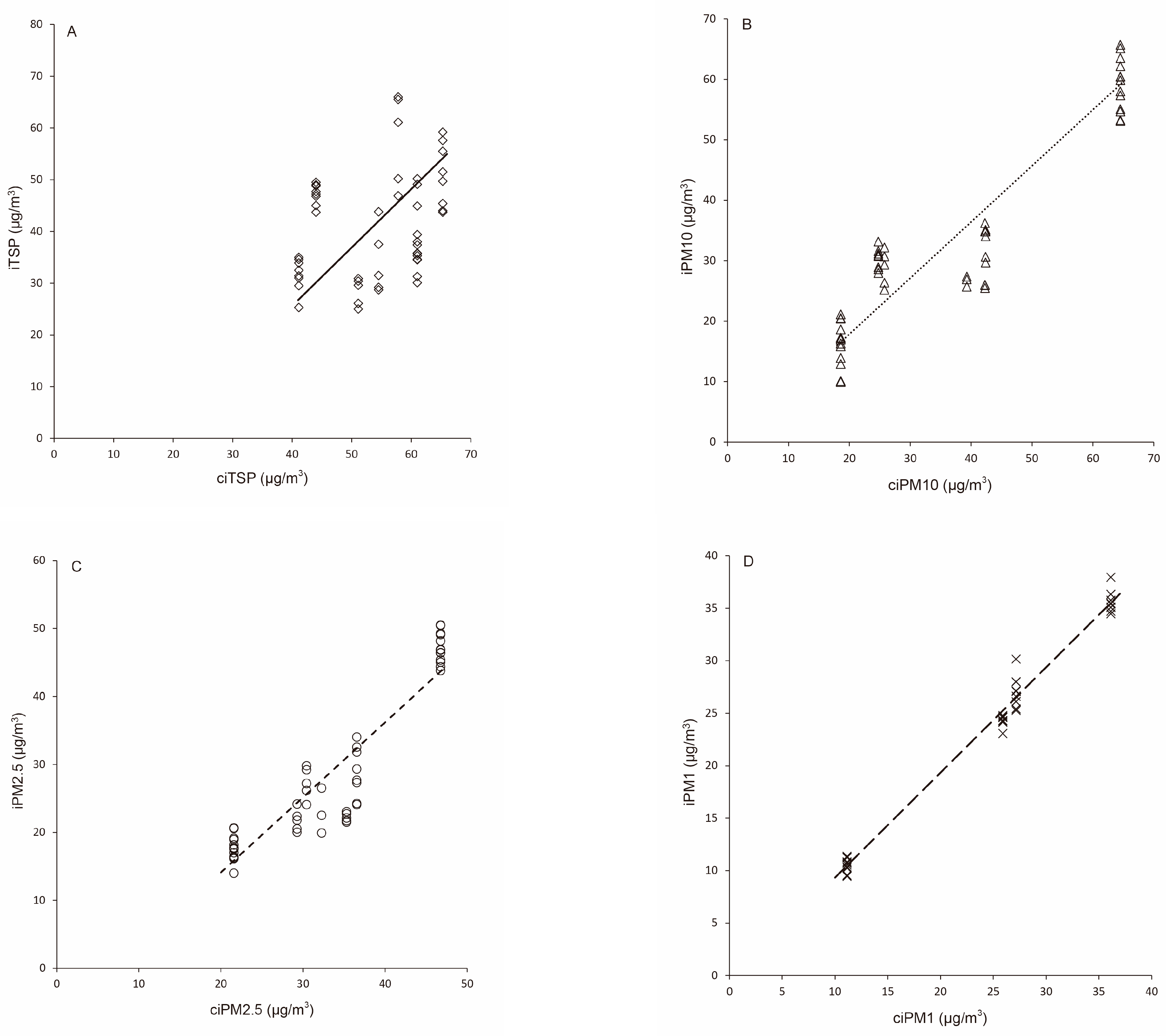
3.3. The Scaling Relationships of iPMs vs. ciPMs at Different Size Levels

The iTSP concentration at the monitoring points was significantly correlated with its control (r² = 0.109, p = 0.017, slope = 1.513 [1.160 1.972] > 1; Figure 3A); the iPM10 was significantly correlated with its control (r² = 0.787, p < 0.001, slope = 1.025 [0.899 1.168] = 1; Figure 3B); the iPM2.5 was significantly correlated with its control (r² = 0.828, p < 0.001, slope = 1.330 [1.183 1.496] > 1; Figure 3C); and the iPM1 was significantly correlated with its control (r² = 0.990, p < 0.001, slope = 1.040 [1.010 1.071] > 1; Figure 3D). The above results at the four size levels show that the iPM concentration increases disproportionately with the increase in the control, except for the one of iPM10 vs. ciPM10, which is proportionally isometric.

Furthermore, the relations between tTSP and ctTSP over different land-use types were also tested. All the relationships were significant, and slope > 1 was included in urban lands (n = 16, r² = 0.959, p < 0.001, slope = 1.453 [1.294 1.632] > 1), forest lands (n = 28, r² = 0.921, p < 0.001, slope = 1.444 [1.289 1.617] > 1), and green lands (n = 8, r² = 0.928, p < 0.001, slope = 1.345 [1.033 1.752] > 1). There was no significant difference (p = 0.820) among the three types of land (n = 56), which had a common slope = 1.435 [1.333 1.550] > 1, and also no significant difference along the x-/y-axis (both p > 0.05). In brief, all the p-values were <0.001 and the slope was >1, indicating that the tTSP concentration in all land-use types accelerated with the increase in control, and there was no significant difference between land-use types.

3.4. The Relationships Between iPM_RR and ciPM

There was a negative correlation in iTSP_RR vs. ciTSP (r = −0.332, p = 0.016; Figure 4A), but there was no significant one in iPM10_RR vs. ciPM10 (r = −0.225, p = 0.108; Figure 4B), and there was a positive correlation both in iPM2.5_RR vs. ciPM2.5 (r = 0.467, p < 0.001; Figure 4C) and in iPM1_RR vs. ciPM1 (r = 0.315, p = 0.023; Figure 4D).

The above results show that the varying tendencies in the relationships of iPM_RR vs. ciPM are different with the increase in ciPM at the different particulate size levels; that is, the iTSP_RR of falling dust decreased with the increase in ciPMs, while the iPM10_RR was not affected, and the iPM_RR below PM2.5 increased. The above serial variations imply that with the particulate size getting smaller, the iPM_RRs change with the increase in ciPM, presenting a trend from declining at the beginning to non-related and then to rising at last. This U-shape-like trend clarifies that with the increase in ciPM concentrations in open space, the averaged reduction effects of lands on the particulates are affected by the size of the iPMs, revealing that the reduction ability over this area gradually increases towards smaller particulate sizes.

4. Discussion

By analyzing the distribution characteristics of PMs with different particle sizes in the Chongqing urban area and examining the relationships among the iPMs and the reduction rate at monitoring points and the scaling relations between iPM and its control, it was found that there were significant correlations in particulates of different sizes, which was consistent with our prediction. Furthermore, the negative correlations between larger-sized falling dust and smaller-sized floating dust were significant, as were the positive ones between fine PMs, the scaling relationship between the iPMs and the control, and the reduction rates varying from decrease to increase with the increase in PMs at control along the decline in particulate size. It is evident that dust deposition can, to some extent, reduce the concentration of floating dust by adsorbing it through gravitational settling. Nevertheless, this conclusion requires further validation. This finding also provides a direction for our future research: conducting controlled laboratory experiments to investigate and verify the underlying mechanism behind the inverse correlation between dust deposition concentration and floating dust concentration.

4.1. The Size Composition of PMs and Its Significance

The proportion of falling dust only accounts for 30%+ of the total concentration, while the floating dust accounts for 2/3; especially PM2.5, which is harmful to a large extent, accounts for 40% both at monitoring points and at control. The above composition structure of PMs in Chongqing city is consistent within the scope of 60–80% observed on the ratio of PM10/TSP. In terms of concentration, PM2.5 is more likely to have an impact on human beings due to its inhalability. Although some scholars have pointed out that population density and temperature have significant effects on the concentration of PM2.5, no comparative analysis has been conducted on its synergy with other inhalable particulate matter.

4.2. The Tradeoff Between Falling and Floating Dusts

There are significant correlations among the concentrations of iPMs with different particulate sizes, indicating that iPM particulates are not independent but interact with each other. The negative correlations between iTSP and iPM10, iPM2.5, and iPM1 indicate that there is a balance between falling and drifting dusts. The underlying mechanisms of this result should be related to the heterogeneous reactions on the surface of particulates with different sizes because the large specific surface area of particulates is an important carrier of atmospheric heterogeneous reactions. As Febo and Perrino found, the production, absorption, and release of chemicals on the surface of particulates depend on the adsorption characteristics on the surface of particulates, while the specific surface area and morphological characteristics of particulates with different particulate sizes vary greatly. The existence of this negative correlation leads us to realize that increasing the concentration of iPMs with large size may reduce the amount of iPM10 and the sub-particulates as well.

4.3. The Scaling Relationship of iPMs vs. ciPMs

The relationships between the iPMs concentration of different particulate sizes and the control show an accelerated increasing trend with the control pollutant, except for the one in iPM10. That is to say, with the increase in iPMs in the control area, the corresponding iPMs in monitoring points are generally faster than control. That is to say, the expansion of urban scale cannot fundamentally control the concentration of pollutants; instead, it deteriorates as the amount of pollutant emissions increases. Furthermore, there is no significant variation in the results of iTSP concentration among three types of urban lands, forest land, and green land, indicating that the above results are not affected by land use types, and the result is analogous to a recently observed phenomenon that the amount of gaseous pollutants has no difference between tree-covered and open areas [29]. This result further confirms the validity from another aspect that the PMs pollution should be controlled from the root cause with emission.

4.4. The Positive Feedback Relations Between Fine Particulates with Different Sizes

The positive correlations among the iPM10, iPM2.5, and iPM1 indicate that as long as one of the pollution concentrations increases, the other two will rise. The positive correlation between fine particulates shows that the association between fine particulates is not like the negative feedback one between falling and drifting dust [30]. The phenomenon is similar to that observed by scholar in that heterogeneous chemistry was enhanced by the aggravation of pollution of three different particulate sizes, which mechanism is interpreted as related to the evolution of key chemical components in PM2.5. We believe that this is an important feature in the prevention and control of air pollution, implying that the increase in one kind of pollutant not only raises itself, but also does the other two. This is a terrible circle effect linked to the fine PMs.

4.5. Relationship Between Reduction Rate and ciPM Concentration with Different Particulate Sizes

The reduction rate of iPMs with different sizes at the monitoring point fluctuates greatly with the increase in the concentration at control, which changes from decrease to increase with a turning point at the intermediate size of iPM10 (Figure 4A–D). The possible causes for that, firstly, the reduction rate of iTSP drops with its control’s increase, may be related to the plant communities’ dust reduction capacity for different particulate sizes as TSP > PM10 > PM2.5 (p < 0.05, this experimental observation), and the main retardation source for TSP is broad-leaved trees [31]. The stomata and glandular hairs of broad-leaved leaves are easily filled and blocked by large-sized particulates, and some of them are not washed off by rainwater and thus fall off from the leaves under external forces to form a kind of secondary pollution source. Therefore, the reduction of iTSPs in large sizes at the monitoring area is declining, especially when the iTSP concentration exceeds a certain limit [32]. Instead, the control sites in the open space are not affected by this change.

Second, the one of iPM10 stays at the turning point from decline to rise, and this may be because the particulate size of iPM10 is in the middle between iTSP and iPM2.5 such that it is not affected by gravity and floats in the air for a long time, so their variations of reduction capacity stemming from plant communities are relatively weak [33,34].

Thirdly, the positive correlation between the reduction rates of iPM2.5 and iPM1, presumably because tPM2.5 is mainly absorbed by coniferous forests in the landscape [35], and our results and accumulated in pine needles as observed by [36]. Maybe the resin secretion of pine needles has a much stronger adsorptive stability to fine particulate sizes of PMs [37] compared to iTSPs, which are detained chiefly by the outer surface of broad-leaved leaves, thus avoiding secondary pollution falling from the leaves [38]. As long as the concentration of iPM2.5 and iPM1 does not exceed a certain threshold, it is normal to absorb more as the concentration increases.

5. Conclusions

In summary, there are size-dependent relationships among the amount of iPMs in urban areas, showing a trade-off between falling and floating dust, a positive feedback among fine particulates, an acceleration model between the iPMs to control, and a U-shaped-like tendency in reduction rate to ciPMs, accompanied by a gradient of particulate size getting smaller. These different correlations imply different changing rules and trends among different particulate sizes of iPMs, which provide a theoretical basis for guiding the prevention and control of PM pollution and its secondary pollutants. The specific research conclusions are as follows:

(1)

Changing land use types have been shown to be ineffective in controlling the concentration of inhalable particulate matter (PM) in urban areas. The study reveals no significant differences in PM concentrations or their mutual constraints across various land use types. Consequently, merely increasing green space ratios is insufficient for urban air pollution control. Instead, effective pollution source management is essential to curb the spread and deterioration of urban air pollution.

(2)

This study elucidates the complex interactions among particulate matter of different sizes. A vicious cycle mechanism exists where an increase in one size of PM can exacerbate the concentration of other sizes. However, there are also beneficial mechanisms that can be harnessed for urban pollution control, such as enhancing the concentration of larger-sized PMs to adsorb and settle smaller-sized particles, thereby contributing to improved air quality. Of course, the above conclusion is merely based on the current observational studies, which lack corresponding experimental verification. This is also the work that we will undertake in the future.

(3)

Open spaces, with their extensive area and land coverage, demonstrate a more pronounced role in reducing particulate matter, particularly in mitigating smaller-sized PMs. Therefore, when addressing air pollution dominated by smaller-sized PMs, leveraging the advantageous mechanisms of open spaces can significantly enhance pollution control efforts.

(4)

Through a combination of field measurements and data analysis, this study clarifies the interactions among particulate matter of varying sizes in the atmosphere. These findings provide precise and actionable strategies for urban pollution control and offer a robust methodological framework for global air pollution research.

References

1. Zhang, X.; Zhang, S.; Lu, J.; Li, R.; Lin, X.; Gao, W. Isotopic characteristics and sources of suspended particulate organic matter in a reservoir of Chinese desert grassland areas: The influence of dry and wet seasons and the role of atmospheric deposition. Environ. Sci. Pollut. Res. 2023, 30, 39042–39054. [Google Scholar] [CrossRef]
2. Wang, W.; He, Q.; Gao, K.; Zhang, M.; Yuan, Y. Spatiotemporal Trends and Influencing Factors of PM2.5 Concentration in Eastern China from 2001 to 2018 Using Satellite-Derived High-Resolution Data. Atmosphere 2022, 13, 1352. [Google Scholar] [CrossRef]
3. Usman, F.; Zeb, B.; Alam, K.; Valipour, M.; Ditta, A.; Sorooshian, A.; Roy, R.; Ahmad, I.; Iqbal, R. Exploring the Mass Concentration of Particulate Matter and Its Relationship with Meteorological Parameters in the Hindu-Kush Range. Atmosphere 2022, 13, 1628. [Google Scholar] [CrossRef]
4. Song, T.; Feng, M.; Song, D.; Liu, S.; Tan, Q.; Wang, Y.; Luo, Y.; Chen, X.; Yang, F. Comparative Analysis of Secondary Organic Aerosol Formation during PM2.5 Pollution and Complex Pollution of PM2.5 and O3 in Chengdu, China. Atmosphere 2022, 13, 1834. [Google Scholar] [CrossRef]
5. Sharma, M.; Kumar, N.; Sharma, S.; Jangra, V.; Mehandia, S.; Kumar, S.; Kumar, P. Assessment of Fine Particulate Matter for Port City of Eastern Peninsular India Using Gradient Boosting Machine Learning Model. Atmosphere 2022, 13, 743. [Google Scholar] [CrossRef]
6. Baltensperger, U. Spiers Memorial Lecture Introductory lecture: Chemistry in the urban atmosphere. Faraday Discuss. 2016, 189, 9–29. [Google Scholar] [CrossRef] [PubMed]
7. Wesener, A. Feeling and interpreting the changing streetscape: Capturing experiences of urban atmospheres in Cuba street, Wellington. Emot. Space Soc. 2024, 52, 101027. [Google Scholar] [CrossRef]
8. Yuan, Y.; Chen, X.; Cai, R.; Li, X.; Li, Y.; Yin, R.; Li, D.; Yan, C.; Liu, Y.; He, K.; et al. Resolving Atmospheric Oxygenated Organic Molecules in Urban Beijing Using Online Ultrahigh-Resolution Chemical Ionization Mass Spectrometry. Environ. Sci. Technol. 2024, 58, 17777–17785. [Google Scholar] [CrossRef]
9. Hoffman, S.; Jasinski, R. The Use of Multilayer Perceptrons to Model PM2.5 Concentrations at Air Monitoring Stations in Poland. Atmosphere 2023, 14, 96. [Google Scholar] [CrossRef]
10. Gao, C.; Liu, M. The Impact of Local Environment and Neighboring Pollution on the Spatial Variation of Particulate Matter in Chinese Mainland. Atmosphere 2023, 14, 186. [Google Scholar] [CrossRef]
11. GB3095-1996; Environmental Air Quality Standard’ promulgated. Environmental Protection Department: Beijing, China, 1996.
12. Li, Y.; Zhang, Z.; Xing, Y. Long-Term Change Analysis of PM2.5 and Ozone Pollution in China’s Most Polluted Region during 2015–2020. Atmosphere 2022, 13, 104. [Google Scholar] [CrossRef]
13. Osbourne, A.; Cante, F. Convivial atmotechnics: Animating atmospheres of togetherness and indeterminacy in Kingston and Abidjan. Environ. Plan. D Soc. Space. 2025. [Google Scholar] [CrossRef]
14. Kosmopoulos, G.; Salamalikis, V.; Matrali, A.; Pandis, S.N.; Kazantzidis, A. Insights about the Sources of PM2.5 in an Urban Area from Measurements of a Low-Cost Sensor Network. Atmosphere 2022, 13, 440. [Google Scholar] [CrossRef]
15. Paiva, D. The paradox of atmosphere: Tourism, heritage, and urban liveability. Ann. Tour. Res. 2023, 101, 103600. [Google Scholar] [CrossRef]
16. Amnuaylojaroen, T.; Surapipith, V.; Macatangay, R.C. Projection of the Near-Future PM2.5 in Northern Peninsular Southeast Asia under RCP8.5. Atmosphere 2022, 13, 305. [Google Scholar] [CrossRef]
17. Bautista, A.; Velasco, F.; Guzmán, S.; de la Fuente, D.; Cayuela, F.; Morcillo, M. Corrosion behavior of powder metallurgical stainless steels in urban and marine environments. Rev. De Metal. 2006, 42, 175–184. [Google Scholar] [CrossRef]
18. Bui, Q.T.; Nguyen, D.L.; Bui, T.H. Seasonal Characteristics of Atmospheric PM2.5 in an Urban Area of Vietnam and the Influence of Regional Fire Activities. Atmosphere 2022, 13, 1911. [Google Scholar] [CrossRef]
19. Bullo, M.; Lakkis, G.; Pustilnik, M.; Bonfiglio, J.I.; Di Pasquale, R.; Gonzalez, L.M.; Gonzalez-Aleman, G.; Lamas, M.C.; Salvia, A.; Langsam, M.; et al. The Relationship between PM2.5 and Health Vulnerability in Argentina in 2010. Atmosphere 2023, 14, 1662. [Google Scholar] [CrossRef]
20. Eronen, M. Aesthetic atmospheres and their affordances in urban squares. J. Place Manag. Dev. 2024, 17, 257–275. [Google Scholar] [CrossRef]
21. Gao, X.; Ruan, Z.; Liu, J.; Chen, Q.; Yuan, Y. Analysis of Atmospheric Pollutants and Meteorological Factors on PM2.5 Concentration and Temporal Variations in Harbin. Atmosphere 2022, 13, 1426. [Google Scholar] [CrossRef]
22. Han, S.; Um, J. Scavenging Efficiency Based on Long-Term Characteristics of Precipitation and Particulate Matters in Seoul, Korea. Atmos. -Korea 2023, 33, 367–385. [Google Scholar] [CrossRef]
23. Reed, D.E.; Lei, C.; Baule, W.; Shirkey, G.; Chen, J.; Czajkowski, K.P.; Ouyang, Z. Impacts of an urban density gradient on land-atmosphere turbulent heat fluxes across seasonal timescales. Theor. Appl. Clim. 2024, 155, 8557–8566. [Google Scholar] [CrossRef]
24. Kobzeva, T.V.; Dultseva, G.G.; Dubtsov, S.N.; Stekleneva, M.E. Natural and Anthropogenic Sources of Organic Aerosol in the Atmosphere: Kinetics and Mechanism of Formation in the Forest-steppe Zone of West Siberia. Atmos. Ocean. Opt. 2024, 37, 614–619. [Google Scholar] [CrossRef]
25. El Hajj, O.; Hartness, S.W.; Vandergrift, G.W.; Park, Y.; Glenn, C.K.; Anosike, A.; Webb, A.R.; Dewey, N.S.; Doner, A.C.; Cheng, Z.; et al. Alkylperoxy radicals are responsible for the formation of oxygenated primary organic aerosol. Sci. Adv. 2023, 9, eadj2832. [Google Scholar] [CrossRef] [PubMed]
26. Talu, C. ‘The Effect of London’: Urban Atmospheres and Alice Meynell’s London Impressions. Emot. Hist. Cult. Soc. 2022, 6, 96–116. [Google Scholar] [CrossRef]
27. Li, J.; Deqing, Z.; Liang, J.; Guo, T.; Yao, J.; Liu, W. Combustion aerosols and suspended dust with controlled processes in Lhasa: Elemental analysis and size distribution characteristics. J. Environ. Sci. 2023, 148, 591–601. [Google Scholar] [CrossRef]
28. CJJT85-2002; Standard of Urban Green Space Classification. Ministry of Housing and Urban-Rural Development of the People’s Republic of China: Beijing, China, 2002.
29. Abusaada, H.; Elshater, A.; Elrahman, A.S.A. Articulating assemblage theory for salient urban atmospheres in children’s environments. Ain Shams Eng. J. 2021, 12, 2331–2343. [Google Scholar] [CrossRef]
30. Liu, S.; Han, Y.; Wang, P.; Zhang, G.J.; Wang, B.; Wang, Y. More Heavy Precipitation in World Urban Regions Captured Through a Two-Way Subgrid Land-Atmosphere Coupling Framework in the NCAR CESM2. Geophys. Res. Lett. 2024, 51, e2024GL108747. [Google Scholar] [CrossRef]
31. Litvintsev, K.Y.; Dekterev, A.A.; Meshkova, V.D.; Filimonov, S.A. Influence of radiation on the formation of wind and temperature regimes in urban environment. Thermophys. Aeromechanics 2023, 30, 683–694. [Google Scholar] [CrossRef]
32. Lin, J.; Wang, X.; Lin, G. Performance and atmosphere in urban public spaces: Street music in Guangzhou, China. Geogr. Res. 2024, 62, 279–292. [Google Scholar] [CrossRef]
33. Kataoka, H.; Tanaka, K.; Tazuya-Murayama, K.; Yamashita, T.; Nishikawa, J.-I. Effects of Coarse and Fine Atmospheric Particulate Matter on a Mast Cell Line. Yakugaku Zasshi-J. Pharm. Soc. Jpn. 2023, 143, 159–170. [Google Scholar] [CrossRef] [PubMed]
34. Kondratyeva, E.V.; Vitkina, T.I. Effects of atmospheric suspended particulate matter on the immune system. Russ. Open Med J. 2024, 13, e0103. [Google Scholar] [CrossRef]
35. Belgacemi, R.; Baptista, B.R.; Justeau, G.; Toigo, M.; Frauenpreis, A.; Yilmaz, R.; Der Vartanian, A.; Cazaunau, M.; Pangui, E.; Bergé, A.; et al. Complex urban atmosphere alters alveolar stem cells niche properties and drives lung fibrosis. Am. J. Physiol. Cell. Mol. Physiol. 2023, 325, L447–L459. [Google Scholar] [CrossRef] [PubMed]
36. Di Croce, N.; Bild, E. How do urban policies shape atmosphere? A multimethod inquiry of the sonic environment. Urban Res. Pr. 2024, 17, 416–437. [Google Scholar] [CrossRef]
37. Huo, M.; Yamashita, K.; Chen, F.; Sato, K. Spatial-Temporal Variation in Health Impact Attributable to PM2.5 and Ozone Pollution in the Beijing Metropolitan Region of China. Atmosphere 2022, 13, 1813. [Google Scholar] [CrossRef]
38. Jiao, X.; Dong, Z.; Baccolo, G.; Qin, X.; Wei, T.; Di, J.; Shao, Y. Quantifying uranium radio-isotope ratios in riverine suspended particulate matter: Insights into natural and anthropogenic influences in the glacial-fed river system of the NE Tibetan Plateau. J. Hazard. Mater. 2024, 461, 132725. [Google Scholar] [CrossRef]
Figure 1. Study scope and sample points.
Atmosphere 16 00609 g001
Figure 2. The quadrats for different plant communities.
Atmosphere 16 00609 g002
Figure 3. Relationship between iTSP concentration at monitoring point and its control point.
Atmosphere 16 00609 g003
Figure 4. The relationships between iPM_RR and ciPM.
Atmosphere 16 00609 g004
Disclaimer/Publisher’s Note: The statements, opinions and data contained in all publications are solely those of the individual author(s) and contributor(s) and not of MDPI and/or the editor(s). MDPI and/or the editor(s) disclaim responsibility for any injury to people or property resulting from any ideas, methods, instructions or products referred to in the content.