Article

Climatology of the Atmospheric Boundary Layer Height Using ERA5: Spatio-Temporal Variations and Controlling Factors

1
Department of Space Science and Engineering, National Central University, Taoyuan 320317, Taiwan
2
Environmental Research and Information Center, Chang Jung Christian University, Tainan 711301, Taiwan
*
Author to whom correspondence should be addressed.
The draft of this paper was done when SSY was at NCU; SSY is now at CJCU.
Atmosphere 2025, 16(5), 573; https://doi.org/10.3390/atmos16050573
Submission received: 30 March 2025 / Revised: 28 April 2025 / Accepted: 6 May 2025 / Published: 10 May 2025
(This article belongs to the Section Climatology)

Abstract

:
Geophysical processes within the atmospheric boundary layer (ABL) play important roles in the energy, momentum, and particle exchanges in the lower atmosphere. The height of the ABL top (ABL height; ABLH) decides the depth of these ABL processes. To better understand the spatio-temporal characteristics of the ABLH, the present study analyzed 45 years of global ABLH data retrieved from ERA5, in which the ABLH was defined using the bulk Richardson number, and the climatology of the ABLH was investigated. Further, the relationship between the ABLH and meteorological parameters was examined. High near-surface air temperature represents fair weather conditions that favor the ABL evolution, causing a high ABLH. In contrast, high precipitation represents bad weather conditions that restrain the ABL evolution, causing a low ABLH. The present study also studied the effects of synoptic weather systems, ocean–atmosphere interactions, terrains, and monsoon systems on the ABLH. Multiple controlling factors, including synoptic systems, cold ocean currents, terrain, and monsoons, influence the weather conditions and the complicated spatio-temporal distribution of the ABLH.

1. Introduction

The atmospheric boundary layer (ABL), also named the planetary boundary layer (PBL), is the bottommost part of the troposphere. The air near the ground surface is affected by radiative heating and cooling, as well as by friction between the surface and the atmosphere. These processes result in the physical properties (wind, temperature, humidity, and so forth) being obviously different within and above the ABL [1,2].
On the one hand, radiative heating during the daytime and cooling during the nighttime modify the thermal structure, affecting the atmospheric stability near the ground. On the other hand, surface drag reduces the airflow speed and further causes turbulence within the ABL. As a result, the air within the ABL is well mixed by turbulence during fair-weather daytime. The entrainment zone (EZ) separates the turbulent ABL and the non-turbulent free atmosphere (FA). However, the EZ becomes the capping inversion (CI) during nighttime, and the EZ and CI are both statically stable layers that usually accompany temperature inversion.
The potential temperature and mixing ratio are almost constant with the height within the turbulent mixed layer (ML) during fair-weather daytime, and these features remain as the ML becomes the residual layer (RL) into the night. Moreover, the wind speed is also near constant and slightly weaker than the geostrophic wind speed within the ML during daytime. However, the wind speed becomes inconstant, and supergeostrophic winds (nocturnal jets; the wind speed is faster than the geostrophic wind speed) may occur in the lower part of the ABL during nighttime [2]. The changes in the ABL structure and properties as time moves from daytime to nighttime and nighttime to daytime constitute the evolution, i.e., vertical structure development, of the ABL under fair-weather conditions.
The ABL properties affect the hydrological cycle (including evaporation and condensation), cloud formation, heat and momentum exchange, wind forcing, and so forth in the troposphere [1,2,3,4,5]. Moreover, the ABL can influence the long-term variation in the sea surface temperature (SST) [6]. These geophysical processes are critical for weather and the global climate system [1,2,3]. Meanwhile, the performance of weather and climate models relies on a proper assessment of the geophysical parameters within the ABL [5]. The ABL even shows its significance in imperceptible ways. For example, the thermal currents within the ABL are essential for migrating birds to soar [7,8,9].
The diffusion and propagation of air pollutants are the most important topics in modern ABL meteorology. Vertical exchange of air parcels across the EZ and CI is restrained due to the high atmospheric stability, and hence, pollutants are trapped within the ABL [1,2,3]. The feedback associated with pollutants, especially particulate matter, can reduce the solar heating during daytime and also reduce the emitted cooling of the ground during nighttime, further modifying the ABL properties and its evolution (e.g., [10,11,12,13]). In worst-case scenarios, the pollutant–ABL feedback may enhance the order of severity of air pollution [14].
On the other hand, the horizontal wind speed and the height of the ABL (ABL height; ABLH) determine the efficiency of pollutant diffusion and propagation. The ABLH, also known as the ABL thickness or ABL depth, is the height from the ground to the ABL top, and the ABL top is defined as the middle of the daytime EZ or the nighttime CI. The ABLH is about 200 m to 4 km, depending on the time, place, and meteorological conditions [15,16,17,18,19,20,21,22]. It has a diurnal variation since the radiative heating and cooling, which affects the structure and evolution of the ABL, has a diurnal cycle. In addition, the roughness of the ground surface affects the wind profile near the ground surface. Humidity is also critical to atmospheric stability influencing the ABLH [1,2,3].
The most conventional method for determining the ABLH is using radiosondes [23,24,25,26] or kytoon/tethered balloons [23,27]. The temperature, humidity, and wind profiles at a fixed location can be measured using in situ instruments. Then, the ABLH is usually derived from rapid changes in the vertical gradients of the potential temperature, humidity, or wind speed. The difference in the balloon ascent rate between within and above the ABL is also a good way to derive the ABLH [25]. Other fixed equipment, such as lidars (see a review in [28] and the references therein), wind-profiler radars [29,30,31], sodar [32], and radiometers [33,34], are also commonly used in the history of ABL observations.
However, the difficulty lies in the observations over oceanic areas, though several experiments have been completed on islands using radiosondes [24,35,36,37]. Nowadays, satellites offer good opportunities for people to extend data coverage from land to sea. Therefore, some studies on the ABL properties over oceanic areas have been performed using lidar [38], radar [15], infrared sounders [39,40], GPS radio occultation (GPSRO) instruments [18,19,22,41,42], and so forth onboard satellites.
Atmospheric reanalysis datasets can provide global data with high spatio-temporal resolution and quality. In the past decade, several studies used ERA-Interim, which is an atmospheric reanalysis dataset produced by the European Centre for Medium-Range Weather Forecasts (ECMWF), as the main data source or the comparative one to study the ABL properties (e.g., [19,21,22,43]). The parameter “boundary layer height” (blh; parameter ID = 159) is not an analysis product but a forecast product in ERA-Interim [44]. Therefore, analysis products, including the temperature, humidity, and wind, were used to derive the ABLH in earlier studies [19,21,43]. A comparison between the native ABLH forecast product and the ABLHs derived from numerous meteorological parameters retrieved from ERA-Interim was made by [21]. The comparison shows that the native ABLH calculated based on the bulk Richardson number is generally lower than the ABLHs derived by other parameters (relative humidity, specific humidity, potential temperature, and so forth; see the complete list in [21]). However, the study [21] supposed that evaluating the correctness among those ABLH results obtained from different methods is difficult due to the lack of reliable observations for the ABLH in a large-scale aspect.
In 2017, the ECMWF released its fifth atmospheric reanalysis dataset, ERA5 [45], next to ERA-Interim. ERA5 uses the same method as ERA-Interim based on the bulk Richardson number to determine the ABLH (see details in Section 2). Nevertheless, the parameter blh becomes an analysis product in ERA5. Similar to the use of ERA-Interim, the native ABLH provided by ERA5 was also employed by some studies [46,47,48,49,50]. However, most of these papers used ERA5 ABLH data as the comparative data to validate their results from the main datasets [46,47,48,49]. The rest [50] studied the spatial and temporal properties of the ABLH over the Tibetan Plateau, which is a regional study using ERA5 ABLH data as the main dataset.
As the “blh” parameter becomes an analysis product in ERA5, it shall provide more realistic ABLH features than ERA-Interim. Also, the temporal resolution of the “blh” products is six hours for ERA-Interim but one hour for ERA5. Not to mention that the temporal coverage and revisit period are both much worse for satellite observations. Even though the global climatology of the ABLH has been studied using ERA-Interim or satellite observations (e.g., [18,19,21,22]), global ABLH climatology using ERA5, as the main dataset, is absent from the literature. However, studying the global ABLH climatology using ERA5 is essential since the dataset can provide the most detailed features, which we have never seen before.
Therefore, in this paper, we employed the ABLH during 1979–2023 (45 years) retrieved from ERA5 to investigate the global characteristics of the ABLH. The spatial and temporal variations in the ABLH at the global scale will be introduced first (Section 3). Then, correlation analyses between the ABLH and meteorological parameters will be performed as hints to determine the casual mechanisms of the ABLH variability (Section 4). Following the results of the correlation analyses, we will summarize the controlling factors in the ABLH from the local to global scales at last (Section 5). This paper aims to provide the most detailed climatology of the ABLH that has not been reported before. The investigation into the causes of the ABLH variability can yield the correspondence between weather conditions and the ABLH. Also, this paper is expected to benefit the performance of weather and climate models, since the ABL properties are crucial to may atmospheric physical and chemical processes, as mentioned at the beginning of this section.

2. Boundary Layer Height Retrieved from ERA5

ERA5 [45] is produced by the ECMWF based on its Integrated Forecasting System (IFS) Cy41r2 with a four-dimensional variational (4D-Var) data assimilation scheme. Numerous observations have been assimilated into the system to embody the global atmosphere from 1950 onwards [51]. The dataset has a horizontal resolution of 31 km (about 0.3° in longitude) and an hourly output frequency, and both are much better than the previous ECMWF reanalysis, ERA-Interim, by 79 km and 6 h.
In the present study, we retrieved ERA5 data with a horizontal resolution of 1°. The re-gridding process was performed automatically by the data server at https://cds.climate.copernicus.eu/ (accessed on 6 January 2025) [45]. The 1° resolution shall be enough to investigate the horizontal variation in the ABLH. On the other hand, the 1 h temporal resolution was kept to present the diurnal variation in the ABLH. This study only used the original ERA5 release from 1979 to 2023. The back extension product from 1940 to 1978 is not included.
The single-level instantaneous parameter “blh” with ID = 159, i.e., the boundary layer height in the IFS Cy41r2, is defined as “the lowest level at which the bulk Ri reaches the critical value of 0.25” [52,53], where Ri is the Richardson number. This algorithm has been assessed by [20] as a method suitable for deriving the top height of both stable and convective boundary layers. Moreover, the algorithm can be applied to all radiosonde, numerical model, and reanalysis datasets. Although the ABLH derived using the bulk Richardson number has a negative systematic difference compared to the ABLHs from other methods (as introduced in Section 1; see details in [21]), a good correlation is found between the different methods (e.g., [20,43,46,49]). The calculation of the bulk Richardson number requires the temperature, humidity, pressure, and wind profiles of the atmosphere. The data sources and numbers of observations of these parameters, which were assimilated into the IFS to produce the analyses in ERA5, can be found in [51].

3. General Climatology of the ABLH

The presentation of the results begins with the general characteristics of the ABLH on a global scale. For more transparent and more concise expressions, we define the following terms, including the areas in both the northern and southern hemispheres if not particularly specified.
  • Equatorial region/latitude(s): the area at latitudes less than or equal to 10°.
  • Low latitude(s): the areas at latitudes between 11° and 30°.
  • Mid-latitude(s): the areas at latitudes between 31° and 60°.
  • High latitude(s): the areas at latitudes equal to or greater than 61°.
However, we also use numerics to express a large area to avoid redundant words. For example, using “within ±60° latitude” instead of “equatorial, low-, and mid-latitudes”.
In addition, we use the term “lands” to indicate any kind of land surface, including continents and islands, whereas the term “waters” refers to any kind of water bodies, including oceans, inland seas, and lakes. However, the terms “continents” and “oceans” are also used to specify large-scale land masses (e.g., the Seven Continents) and water bodies (the Five Oceans).
Moreover, we will discuss the spatial variations in the ABLH with different scales from several hundred to thousands of km in this study. We briefly use “global” features/effects to mention those properties that are common over the globe, whereas “local” features/effects mention those properties that only appear in a specific region with a horizontal scale of hundreds to thousands of kilometers. The term “local” is a relative expression to “global”, and no particular size of its scale is defined.

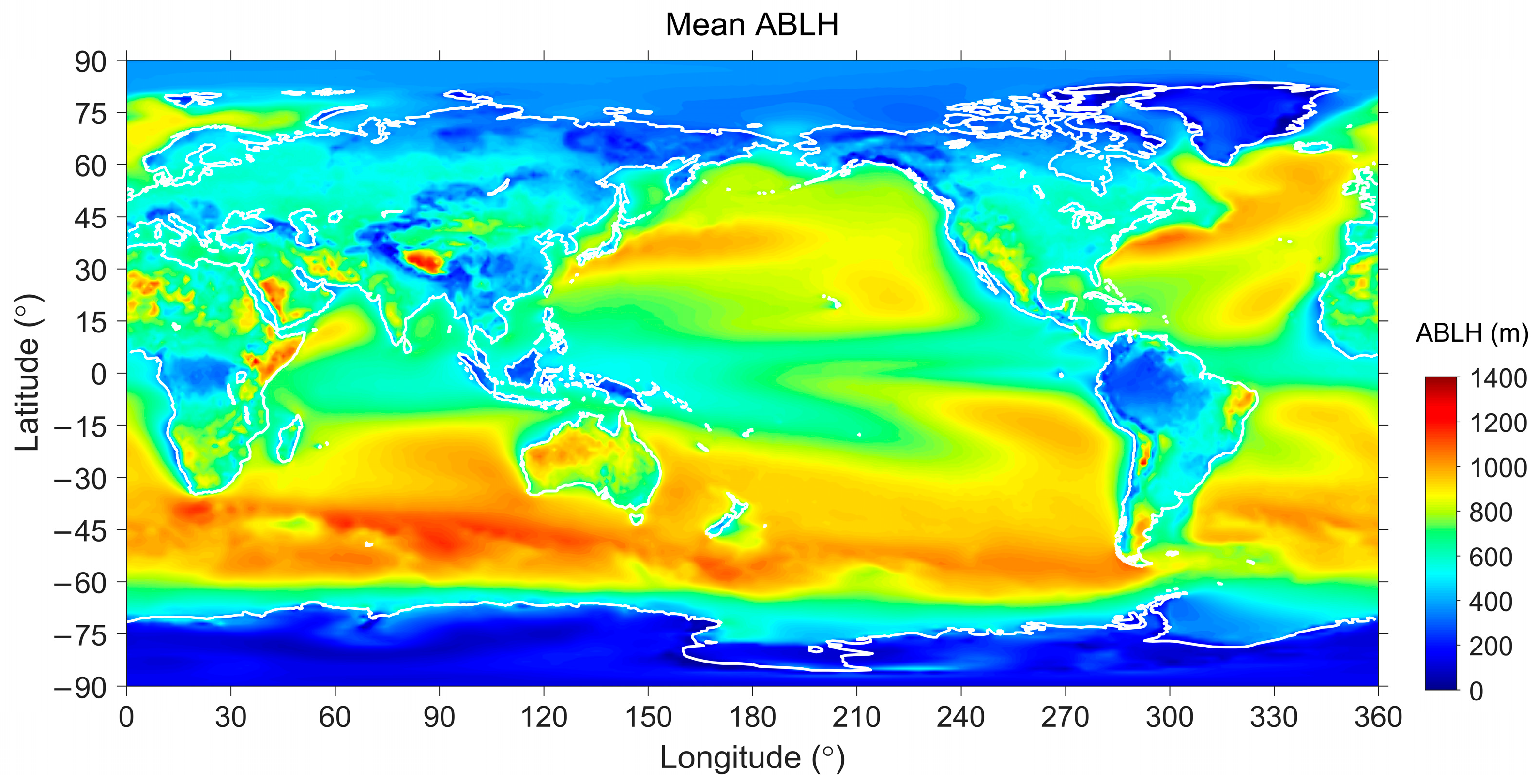
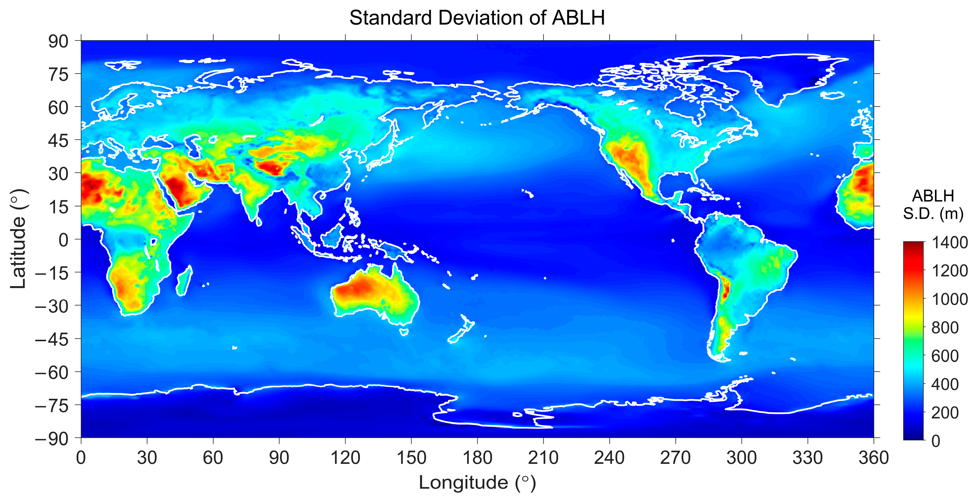
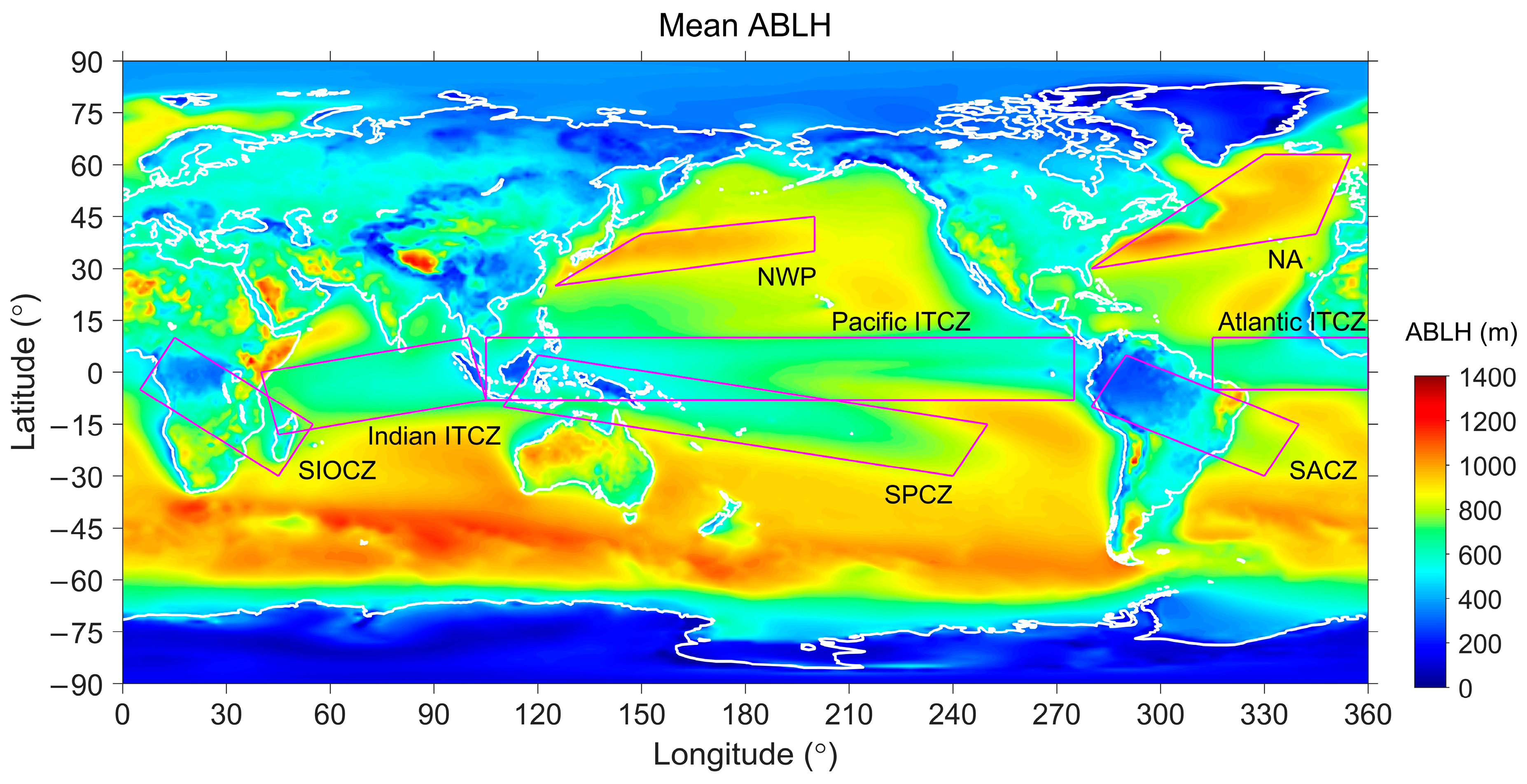
3.1. Long-Term Mean ABLH

Figure 1 shows the global ABLH above ground level (AGL) averaged during the 45 years from 1979 to 2023. All the values from 24 local hours were averaged, and therefore, this figure only shows the spatial variation in the ABLH. The mean ABLH distributes from several tens of meters over Antarctica to about 1280 m over the southern mid-latitude Indian Ocean. The mean ABLH is generally much lower over lands than waters (global mean: 417 m vs. 750 m).
Figure 2 shows the standard deviation, i.e., the temporal variability, of the ABLH over the globe. The standard deviation of the ABLH is larger over lands than waters (global mean: 423 m vs. 304 m), indicating that the ABLH is more variable over lands than waters. This is reasonable because the temporal variation in the temperature, representing the cumulation of radiative heating, is much more significant over lands than waters. Also, the deviation is larger over low latitudes than over other latitudes.
It is also known from Figure 1 and Figure 2 that the ABLH is relatively low and steady at equatorial and high latitudes. However, the geographic and meteorological conditions of these two places are quite different. Moreover, the ABLH is at an intermediate level but has large variability over low- and mid-latitudinal lands. The standard deviation is even greater than the mean value of the ABLH over these places. By contrast, the mean ABLH is higher, but the variability is much lower over low- and mid-latitude waters.

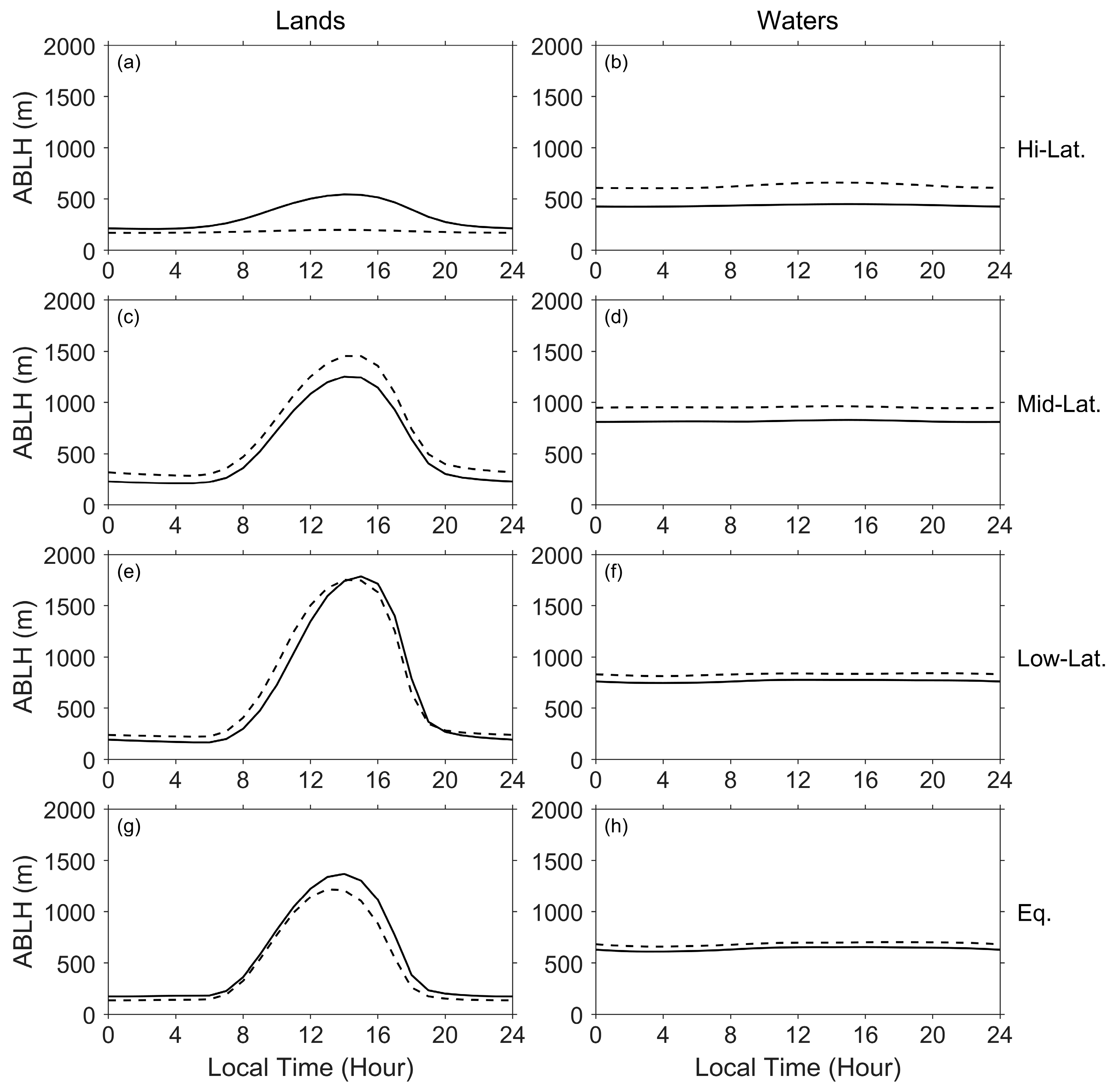
3.2. Diurnal Variation in the ABLH

In this subsection, we discuss the diurnal variation in the ABLH. Hence, the time series of the ABLH in local time (LT) is needed. However, the native ERA5 dataset uses universal time (UT). A conversion from UT to LT was made to construct the results in LT. In the present study, we followed the standard of the nautical time zone, in which the globe is divided into 24 time zones with hourly offsets and 15° spacing in longitude. The time zone in the LT is the same as the UT and runs from −7° to 7° longitude (note that the horizontal resolution taken in this study is 1°), whereas another time zone in which the LT is one hour ahead of the UT runs from 8° to 22° longitude, and so on.
Figure 3 plots the mean ABLHs of the 24 h in LT over different surfaces (lands/waters) and latitudinal sectors. The values in the northern and southern hemispheres are plotted by solid and dashed curves, respectively. Generally, the ABLH is lowest around 4–6 LT before sunrise and highest around 14–15 LT in the afternoon, and both are simultaneous with the extremes of temperature during the day. However, the diurnal variation over waters is obscure. In contrast, the diurnal variation is evident over lands except for the southern high latitudes.
The ABLH over southern high-latitude lands is nearly the same during different local times. Antarctica is the only continent over the southern high latitude, and most of its surface is covered by the Antarctic ice sheet. The lower atmosphere has almost no interaction with the smooth ice surface. In addition, the ice surface can be considered a “white body,” which is almost unaffected by radiative processes, and the diurnal variation in the temperature is insignificant. Therefore, the ABLH over Antarctica is low and steady, having a very different characteristic from the other lands, as seen in Figure 1, Figure 2 and Figure 3.
Over lands except for the southern high latitudes, the nighttime ABLH is about 160–400 m, whereas the ABLH at 14–15 LT ranges from about 550 to 1750 m, depending on the latitude. Since the difference in the nighttime ABLH between different latitudes is relatively few, a higher ABLH during daytime can result in a higher diurnal variability. Both the daytime ABLH and the diurnal variability are highest over low-latitude lands (Figure 3e). It is somewhat beyond our expectation that the theoretical radiative forcing is most potent, but the daytime ABLH is not the highest at equatorial latitudes.

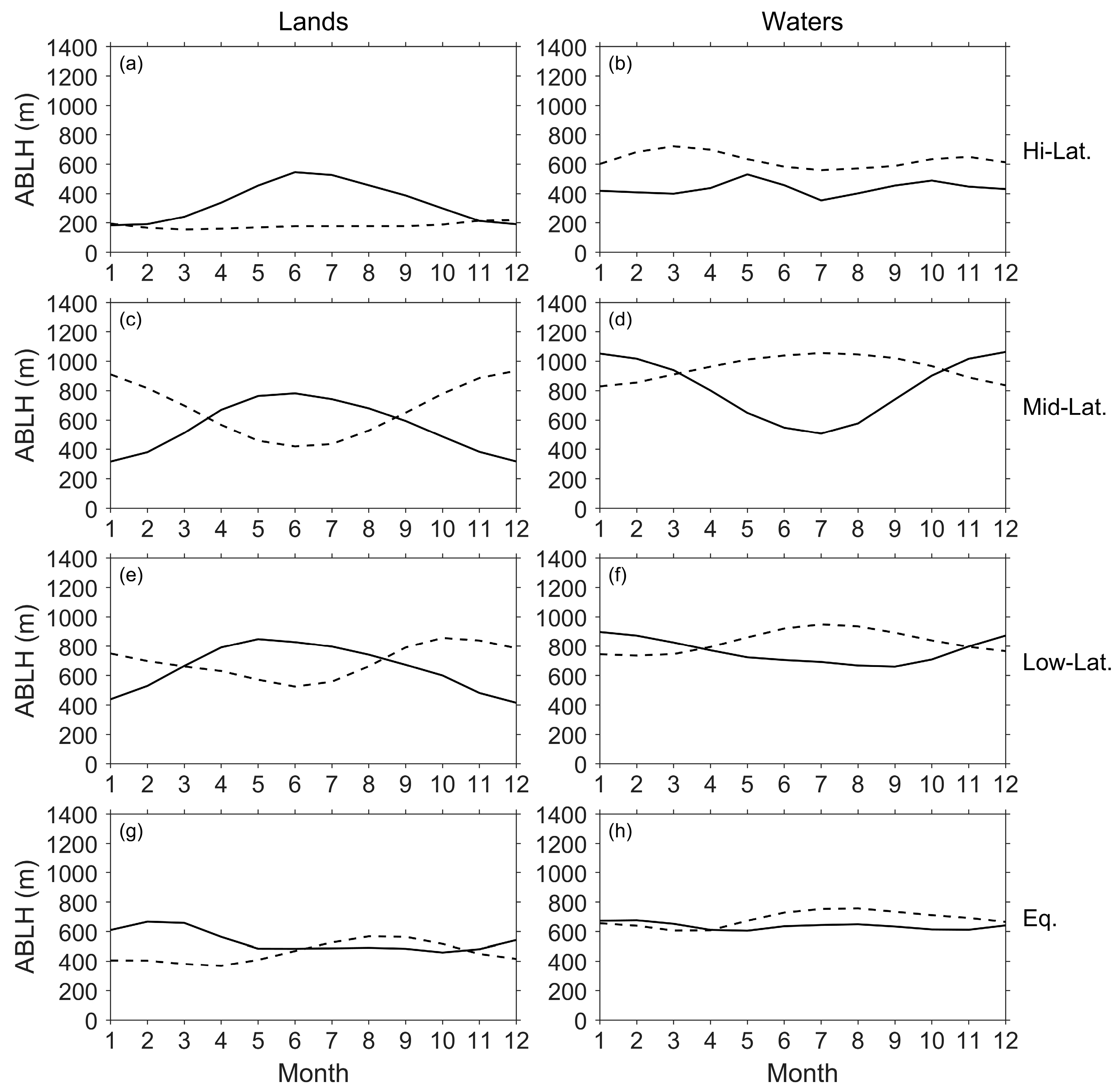
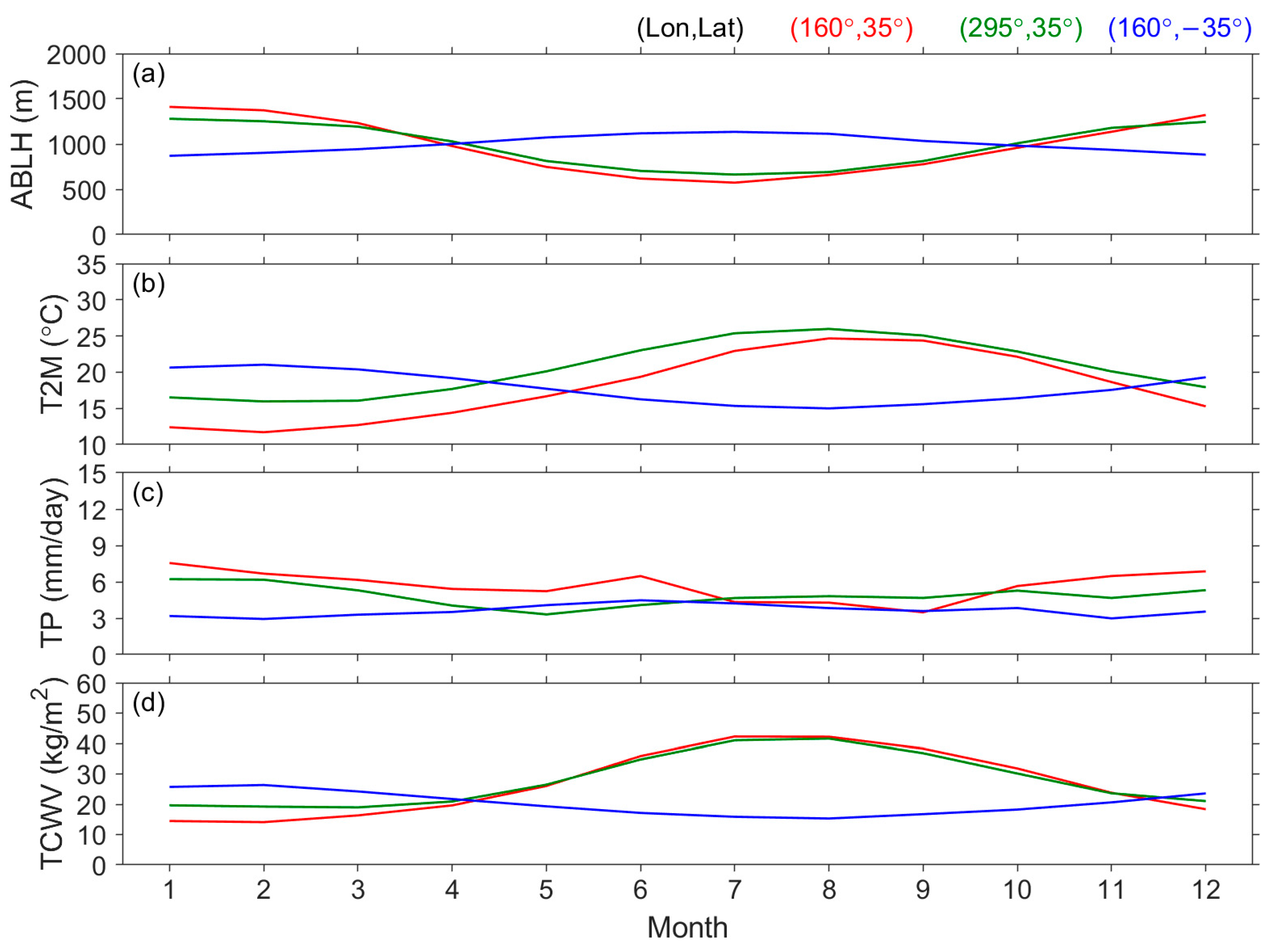
3.3. Seasonal Variation in the ABLH

The 45-year averaged monthly ABLH was also calculated to reveal the seasonal variation over different surfaces and latitudinal sectors, as plotted in Figure 4. The results are the mean values of the 24 local times, and thus, the maximum of each curve in Figure 4 is much smaller than those in Figure 3. In general, the mean ABLH is higher in summer than in winter over lands in both hemispheres except for equatorial latitudes, but it is higher in winter than in summer over the low- and mid-latitude waters in both hemispheres. In other words, the seasonal variations over lands and waters are out of phase at both low and mid-latitudes.
Over the high-latitude waters in both hemispheres, the ABLH is lower not only in summer but also in winter. The nighttime is much longer than the daytime at high latitudes during winter, and the accumulation of radiative heating is much lower in winter than in summer. The ABLH over the high-latitude waters shows another minimum in the winter months due to cold weather.
The ABLH over equatorial latitudes shows an annual cycle with a relatively small magnitude (less than 100 m, peak-to-peak) compared with the other latitudes (about 200–550 m). However, its peak height over lands occurs between winter and spring but not summer (although the terms “summer” and “winter” are not appropriate for the equatorial latitudes, we follow the definition at higher latitudes). The results shall be explained by a proper mechanism. Nevertheless, we retain the question here, and it will be taken up again in Section 5.1.1.
In addition, both the northern and southern high-latitude lands have annual variations in the ABLH. However, the peak-to-peak magnitude is about 390 m over the northern high-latitude lands but only about 60 m over the southern high-latitude lands. The ABL over Antarctica again shows its uniqueness caused by ice sheets.

3.4. Monthly and Hourly ABLH Maps

As the spatial (long-term mean), diurnal, and seasonal variation are independently introduced in Section 3.1, Section 3.2 and Section 3.3, respectively, the monthly and hourly ABLH maps are also plotted in Figures S1–S36. Readers interested in how the ABLH varies with the season (Figures S1–S12) and local time (Figures S13–S36) can refer to the Supplementary Materials of this paper.

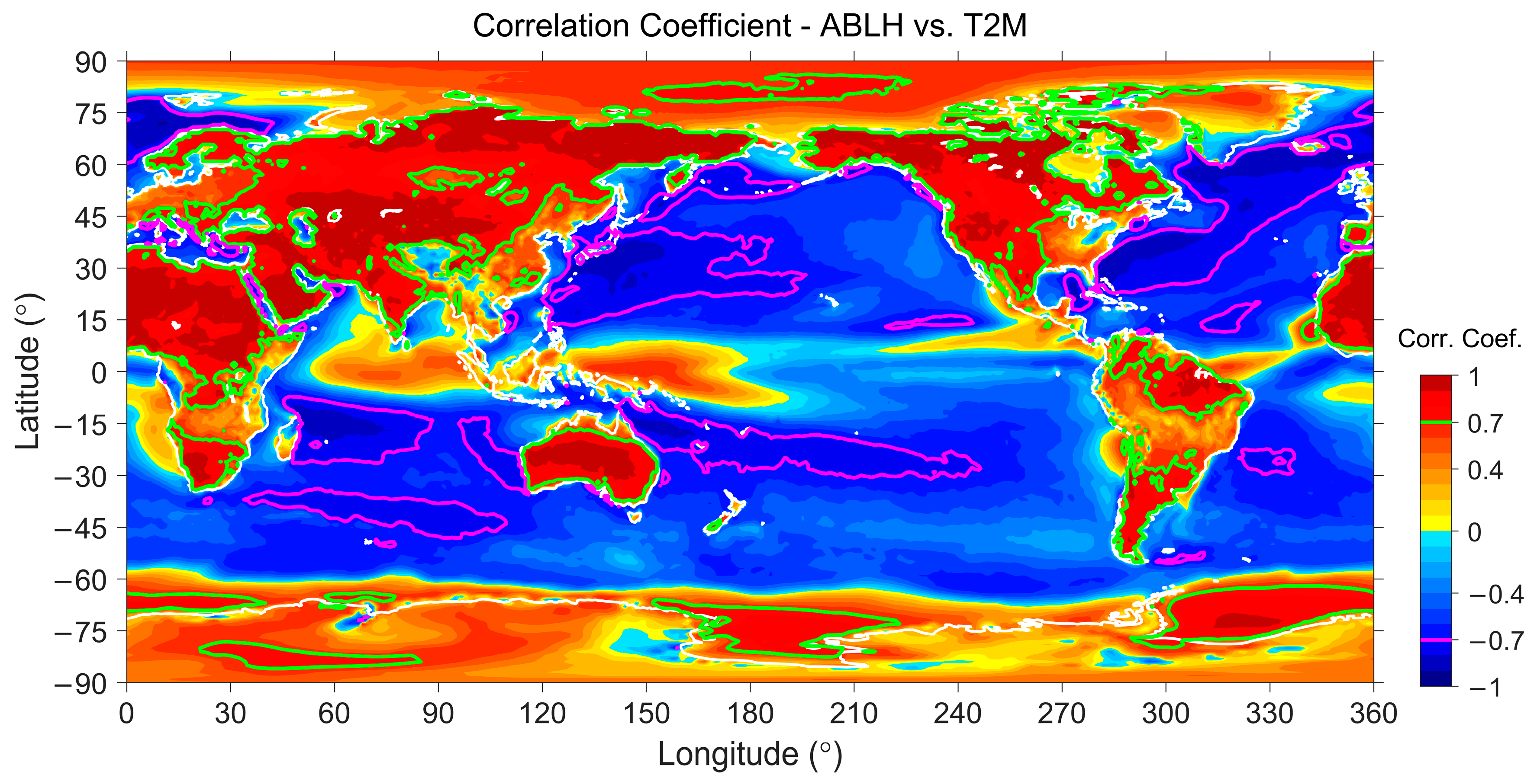
4. Weather Conditions and Correlation Analyses

Figure 1 reveals some local features in which the ABLH is either higher or lower than the neighboring areas. In addition, the variations in the ABLH over lands and waters are out of phase at low and mid-latitudes, as seen in Figure 4. Since the evolution of the ABL relies on radiative heating from the sun and cooling by the ground [1,2,3], the weather conditions shall be examined and compared with the ABLH to find out the mechanisms that cause the dissimilarity of the ABLH in space (Figure 1) and in time (Figure 4). The results will reveal how the ABLH is affected by weather conditions, providing hints as to the ABLH controlling factors (which will be discussed in Section 5) we are searching for.

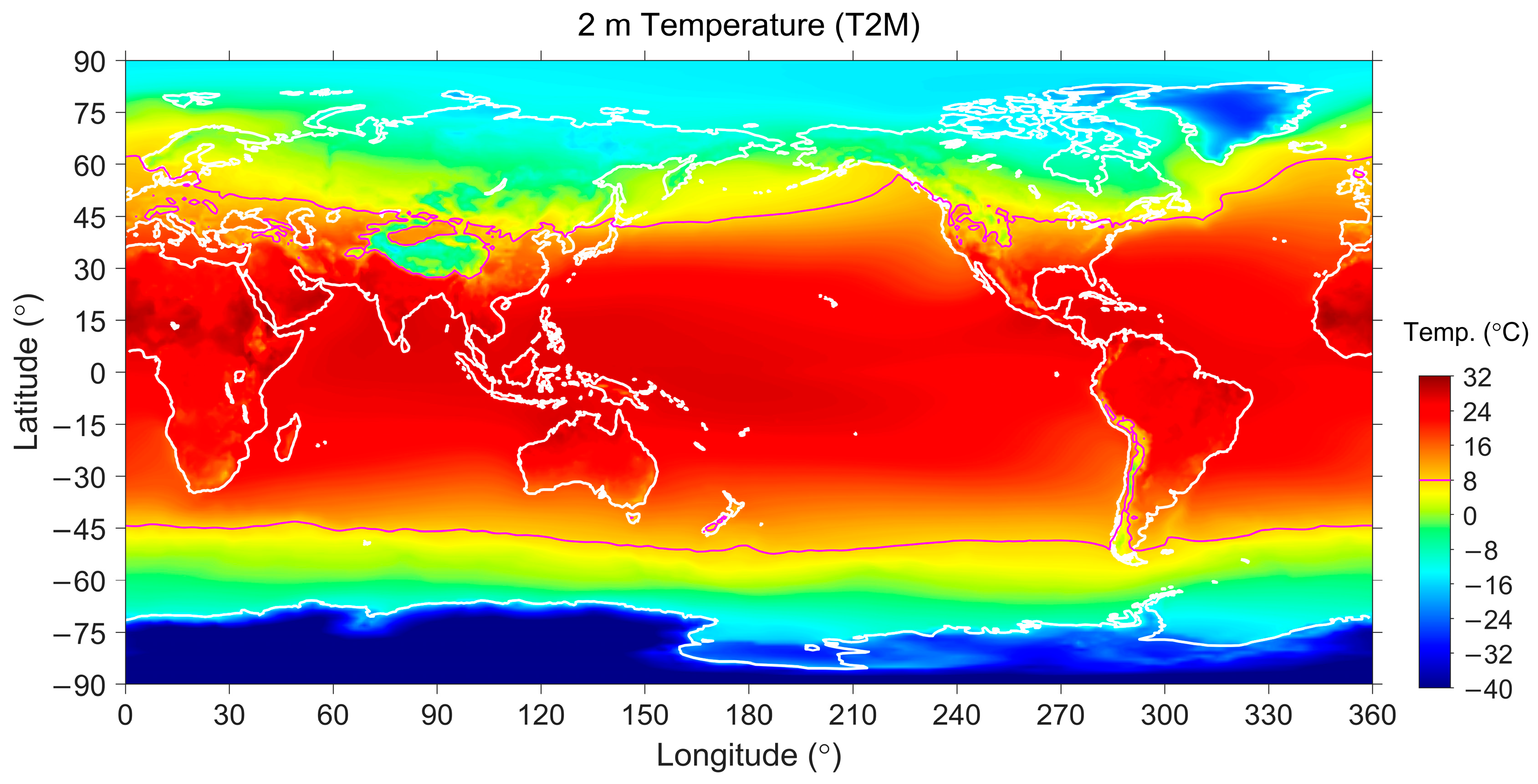
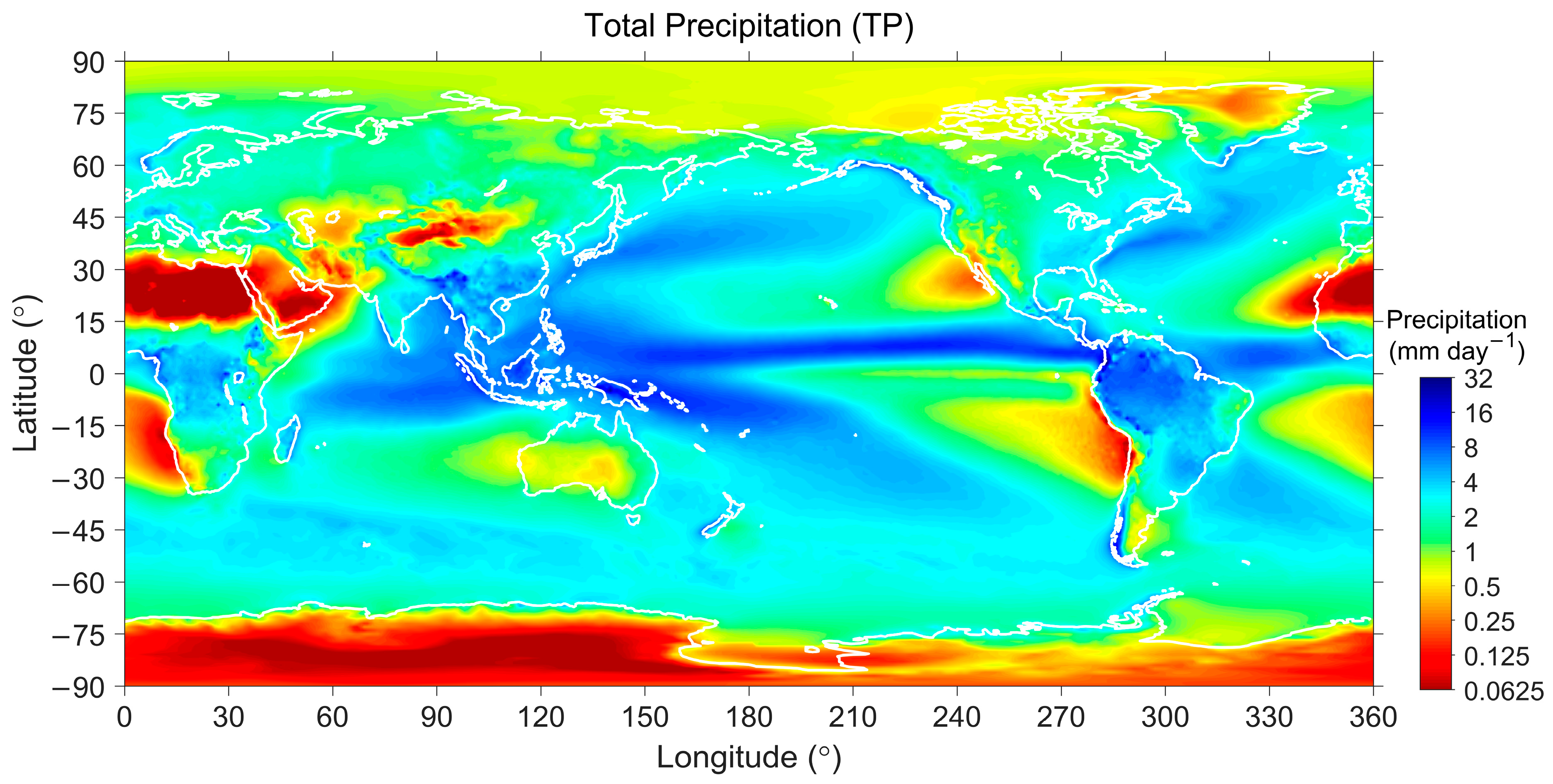
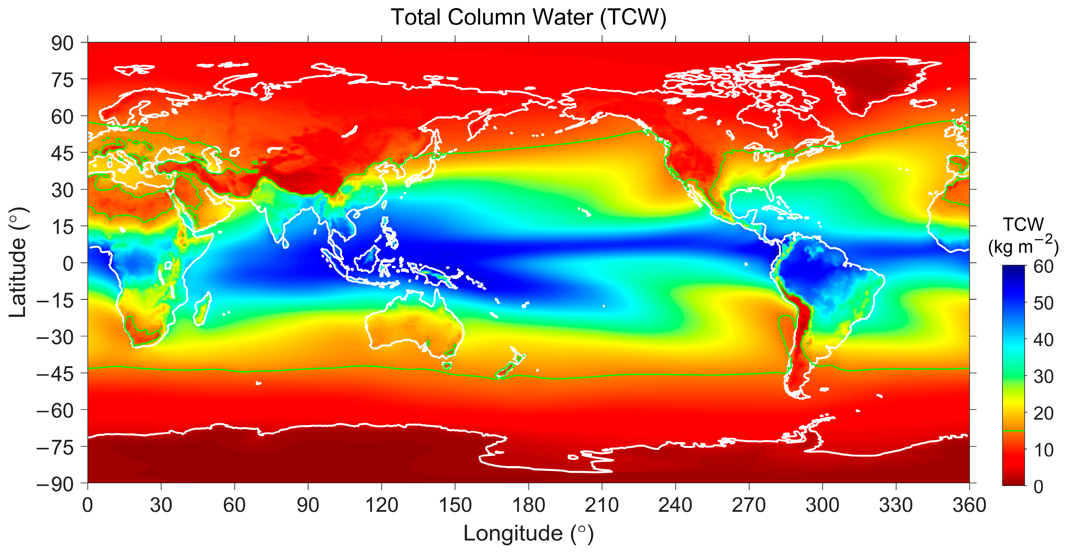
4.1. Meteorological Parameters as Proxies of Weather Conditions

Two basic and one advanced meteorological parameters provided by ERA5 were employed as the proxies of the weather conditions. The first one is the 2 m temperature (parameter “2t” with ID = 167; abbreviated as T2M hereafter). The near-surface air temperature represents the accumulated radiative heating/cooling at the bottom of the atmosphere, which is critical for the evolution of the ABL.
The second one is the total precipitation (parameter “tp” with ID = 228; abbreviated as TP hereafter). During fair-weather daytime, the sun can support radiative heating, favoring the development of thermals in the ABL. However, assessing fair-weather conditions using basic parameters provided by ERA5 or even other conventional instrumental observations is difficult. Nevertheless, the assessment of bad weather conditions is much more accessible through the occurrence of precipitation. With precipitation, the sky is supposed to be obscured by rain clouds, radiative heating from the sun is limited, and the weather is considered unfavorable for the evolution of the ABL.
The last one, the total column water vapor (parameter “tcwv” with ID = 137; abbreviated as TCWV hereafter), was also examined in this study. The TCWV is the vertical integral of the water vapor content above a unit area. A high value of the TCWV reflects that much water vapor accumulates within the vertical column. Once the water vapor condenses, it can form clouds, further resulting in precipitation. On the other hand, the temperature of an air parcel decides the saturation vapor pressure, i.e., how much water vapor can be contained within the air. Therefore, the TCWV mixes the information about precipitation and temperature at the same time, and we employed the TCWV as the third meteorological parameter, which makes it possible to describe the weather conditions.
All three selected parameters were retrieved from ERA5, and the data process procedures were the same as for the ABLH, as mentioned in Section 2. Also, the 45-year mean values of the T2M, TP, and TCWV were calculated using the same method as for the mean ABLH, and the results are plotted in Figure 5, Figure 6 and Figure 7. Be aware that Figure 6 and Figure 7 use a reversed color axis.

4.2. Correlation Analyses: A Short Preface

Some basic and qualitative comparisons can be made by the naked eye by comparing Figure 1, Figure 5, Figure 6 and Figure 7 directly. For example, over the equatorial and low latitudes, the ABLH (Figure 1) and the two parameters of the TP (Figure 6) and TCWV (Figure 7) show respective opposite tendencies. Hence, a reversed color axis design is used in Figure 6 and Figure 7.
However, we need quantitative analyses to obtain more reliable results regarding the effects of the three selected parameters on the variations in the ABLH. For this purpose, correlation analyses, which contain spatial and temporal analyses, were performed.
Each (spatial and temporal) analysis presented a few specific meanings from the results, helping us to determine the causality between the ABLH and meteorological factors. Nevertheless, we mainly focus attention on the procedures for the correlation analyses in this section. The results of the analyses are given. However, only the general properties at the global scale are described. The detailed mechanisms regarding local phenomena will be discussed later in Section 5.

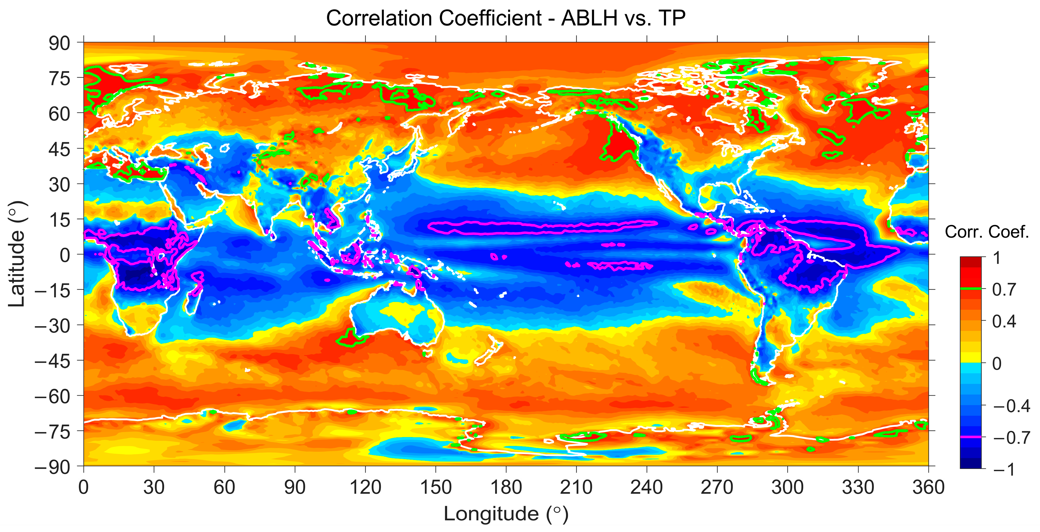
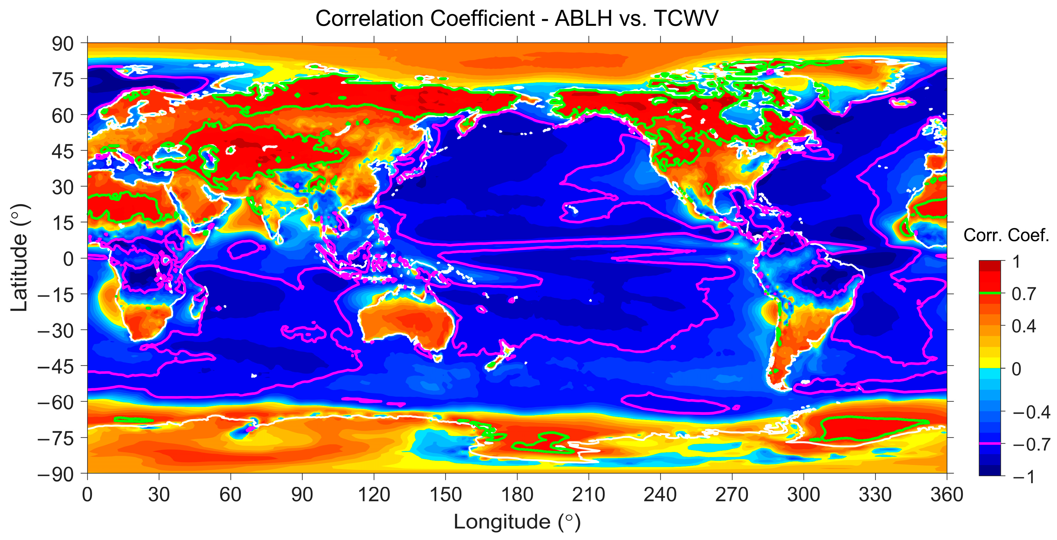
4.3. Spatial Correlation Analyses

The spatial analyses calculated the correlation coefficients ( r ) between the 45-year mean values of the ABLH and selected meteorological parameters at different places. The analyses were performed above different surfaces over the globe and eight latitudinal sections, and the results are summarized in Table 1. The cases of strong (defined as r ≥ 0.7) and moderate (0.7 > r ≥ 0.4) correlations are highlighted with colors. In addition, the scatter plot for each pair from the correlation test is also shown in Figure 8 for reference.

4.3.1. Spatial Analysis Results over Lands

We first look at the results over lands on the global scale. The T2M, TP, and TCWV, respectively, show strong positive, no ( r < 0.1), and moderate positive correlation with the ABLH over the global lands. As expected, the ABLH and T2M are strongly positively correlated ( r = 0.844) because the accumulated radiative heating near the ground surface favors the evolution and vertical development of the ABL. Comparing Figure 1 and Figure 5, the ABLH is roughly higher over the area with a higher T2M. However, the correlation becomes no to moderate when we limit the statistic area to a specific latitudinal section (except for the northern high latitudes). The scatter plot in Figure 8a also reveals that the ABLH tends to be higher as the temperature increases on the global scale. Nevertheless, the data points distribute chaotically for most latitudes, especially within the ±60° latitude.
On the other hand, the ABLH and TP show a very weak correlation ( r = 0.157) over the global lands. However, they show moderate to strong negative correlations over lands within the ±60° latitude and moderate positive correlations over high-latitude lands, respectively. The scatter plot in Figure 8b reveals a chaotic distribution between these two parameters. Nevertheless, the ones within ±60° latitude present their respective negative correlations in each specific latitudinal section, as shown in Table 1.
As the water vapor content is considered to be higher with higher temperature and precipitation, the statistics show that the TCWV is strongly positively correlated to the T2M ( r = 0.822) and TP ( r = 0.705) over the global lands (not listed in Table 1). The analytical results of the TCWV group also seem to be a mixture of the T2M and TP groups (Table 1), showing a moderate positive correlation ( r = 0.558) over the global lands. However, it is not proper to conclude that the ABLH and TCWV have a positive correlation because the scatter plot in Figure 8c reveals that the data points within the plot can be classified into two categories by the threshold of 15 kg m−2 in the TCWV, as indicated by a gray line in the plot. The dry ones on the left-hand side show a strong positive correlation ( r = 0.84), whereas the wet ones on the right-hand side show a moderate negative correlation ( r = −0.46). Since most of the dry/wet ones are distributed over higher/lower latitudes geographically (Figure 7 and Figure 8c), the positive/negative correlations are also seen in the higher/lower latitude sections in Table 1.
In addition, the results over lands (Table 1 and Figure 8a–c) reveal that the T2M and TP are the critical parameters that correlate with the ABLH over higher/lower latitudes, respectively. It seems that bad weather conditions (high TP) reduce the ABLH over lands within ±60° latitude, and fair weather conditions (high T2M) elevate the ABLH over high-latitude lands.

4.3.2. Spatial Analysis Results over Waters

Turning to the results over waters, the ABLH and T2M have a correlation coefficient of 0.455 over the global waters. However, the ABLH and T2M show either no or weak negative correlations over waters within ±60° latitude but strong positive correlations over high latitudes. Similar to Figure 8c, the data points within Figure 8d can be roughly classified into two groups by 8 °C in the T2M. The ones on the left-hand side show a strong positive correlation ( r = 0.897), whereas the ones on the right-hand side show a moderate negative correlation ( r = −0.621).
Similar to the results over lands, the ABLH and TP are weakly correlated ( r = 0.195) over the global waters. In particular, they are negatively correlated over waters within ±30° latitude but positively correlated without ±30° latitude.
The results of the TCWV group are very similar to those of the TP group over waters. Nevertheless, all the T2M, TP, and TCWV groups over waters have correlation coefficients with the same sign in each latitudinal section. An exception is over the southern mid-latitude waters, and the ABLH there is moderately positively correlated to the TP but not correlated to the T2M and TCWV. The same 15 kg m−2 threshold can be used to classify the data points within Figure 8f into two categories. The dry ones show a strong positive correlation ( r = 0.752), whereas the wet ones show a strong negative correlation ( r = −0.705).
As revealed by the results over waters in Table 1 and Figure 8d–f, the ABLH over waters within ±60° latitude seems mainly affected by bad weather conditions; however, over mid-latitude waters, the ABLH is higher over high TP areas (positive correlation), which is much different than that over mid-latitude lands.

4.3.3. Short Summary of the Spatial Analyses

In summary, the T2M presents the spatial variation in the ABLH well over higher latitudes, as well as the TP over lower latitudes. The TCWV contains information from both the temperature and the precipitation, so it can be a good proxy to represent the weather conditions critical to the evolution of the ABL. The results of the spatial correlation analyses suggest that (1) the ABLH is mainly dominated by the near-surface air temperature with a positive correlation under the dry condition (the time-averaged TCWV is less than 15 kg m−2); and (2) the ABLH is mainly dominated by the precipitation with a negative correlation under the wet condition (the time-averaged TCWV is greater than 15 kg m−2).

4.4. Temporal Correlation Analyses

The 45-year time series of the ABLH, T2M, TP, and TCWV within each 1° × 1° grid were retrieved from ERA5. The temporal analyses calculated the correlation coefficients between the time series of the ABLH with the T2M, TP, and TCWV. The calculation was performed within each grid cell over the globe, and therefore, the results of the temporal analyses can be illustrated with figures. Before showing the results, we have to mention again here that this section only concerns the general characteristics of the ABLH and the relevant correlation results on a global scale. The local effects will be discussed later in Section 5.
First, we look at the results of the temporal analyses between the ABLH and the T2M in Figure 9. In general, the ABLH and T2M are positively correlated over lands. Especially over the areas with less precipitation (Figure 6), the corresponding correlation coefficients are usually greater than 0.7, indicating a strong correlation between the ABLH and the T2M over lands. On the other hand, the ABLH is generally negatively correlated to the T2M over waters. It is also seen in Figure 4 that the ABLH over the low- and mid-latitude waters is higher in winter than in summer. However, the correlation coefficients over the equatorial and high-latitude waters are positive, different from the low- and mid-latitude waters.
Figure 10 shows the results of the temporal analyses between the ABLH and the TP. In general, negative and positive correlations are found over lower and higher latitudes, respectively, in both hemispheres. The transition from negative to positive correlation, i.e., zero correlation, occurs around ±30° latitude over waters but reaches around ±45° latitude over lands. Anomalies are found in some areas over the equatorial and low-latitude areas, e.g., the Arabian Sea and the southern margin of the Sahara.
The results of the TCWV (Figure 11) seem to be a composition of the results of the T2M and TP (Figure 9 and Figure 10). In general, it shows positive correlations over lands, as the ABLH and T2M are positively correlated over lands (Figure 9), and the T2M is one of the major controlling factors of the TCWV. By contrast, negative correlations are found over waters, as the ABLH is negatively correlated to either the T2M or TP depending on the latitude over waters (Figure 9 and Figure 10). It also shows strong negative correlations over lands with intense precipitation within ±15° latitude. Bad weather restrains the vertical development of the ABL, and low ABLH is observed here.

5. Controlling Factors of the ABLH

We have figured out some general rules regarding the characteristics and variations in the ABLH at the global scale in Section 3 and Section 4. In this section, we turn to the local factors, which can affect the ABLH with horizontal scales of hundreds to thousands of kilometers. For these factors, symbolic examples will be demonstrated with the 45-year averaged monthly means of the ABLH, T2M, TP, and TCWV. The demonstrations and the results reported in Section 3 and Section 4 can lend us a clear view to understand the role of these local effects on the variations in the ABLH.

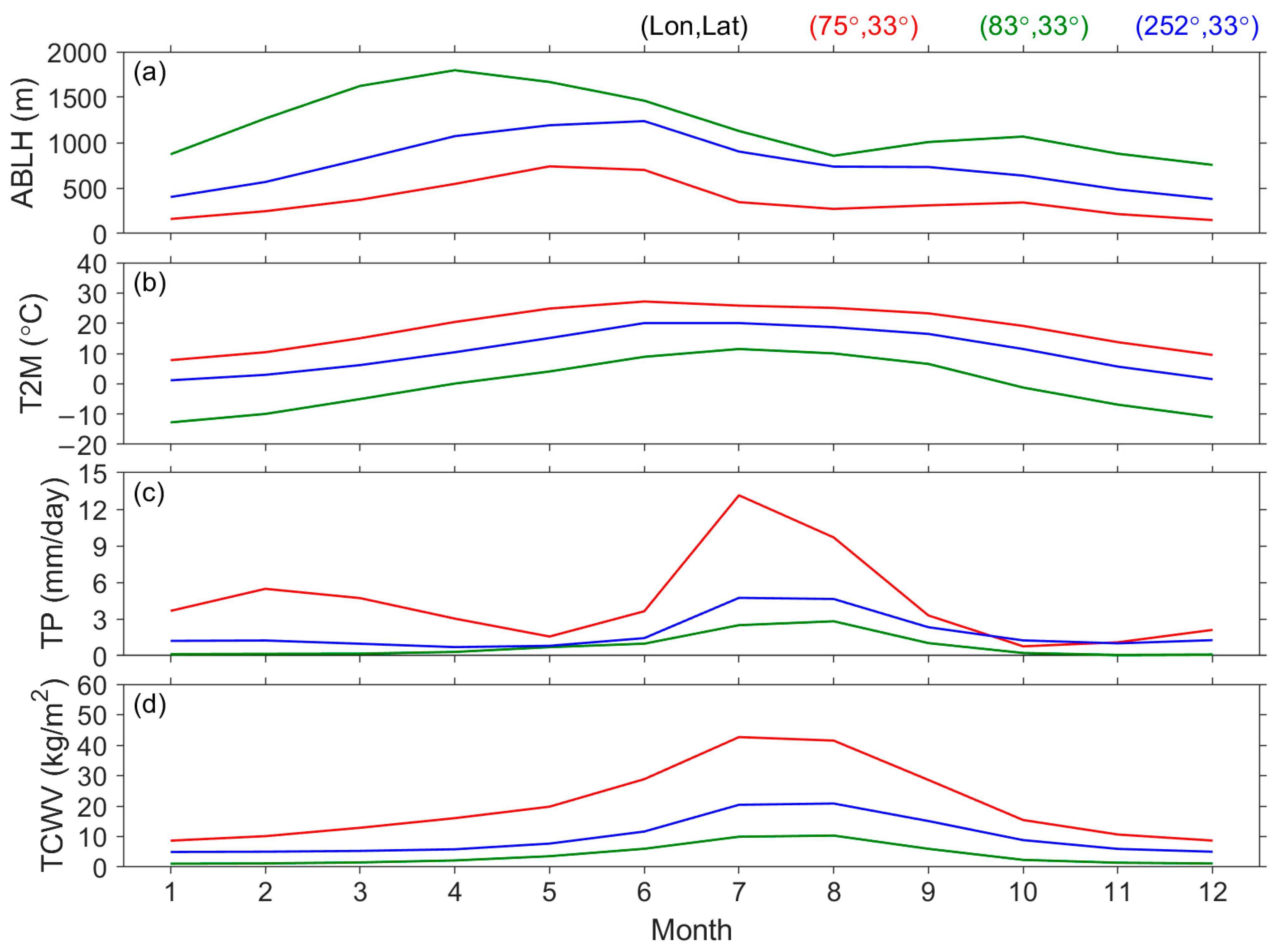
5.1. Synoptic-Scale Weather Systems

As weather conditions play a crucial role in the evolution of the ABL, synoptic-scale weather systems are considered to affect the ABLH over a wide region at the horizontal scale, which is the same as these systems. Figure 12 maps the mean ABLH again, as shown in Figure 1, and further indicates some areas of interest in which the ABLH may be affected by synoptic-scale weather systems.

5.1.1. Convergence Zones

There are two low ABLH regions over the equatorial and southern low-latitude Pacific (Figure 12). One is almost right over the equator, and another one originates in the Indonesian region, extending southeastward to about 240° longitude and −25° latitude. Their pattern on the map is often seen in the plots of meteorological and oceanic parameters, such as the precipitation (Figure 6) and SST. It is correlated to the convergence zones (CZs) over the Pacific Ocean; specifically, the intertropical convergence zone (ITCZ) [54] and the South Pacific convergence zone (SPCZ) [55,56]. The region influenced by the ITCZ extends to the Indian Ocean and actually encircles the global equatorial region as the ITCZ is essentially driven by the global tropospheric circulation (nevertheless, only the parts of the ITCZ over oceans are indicated in Figure 12).
In addition, there are two minor CZs in the southern hemisphere. One is the South Atlantic convergence zone (SACZ), which originates in the Amazon basin and extends southeastward toward the South Atlantic Ocean [57,58]. The other one is the South Indian Ocean convergence zone (SIOCZ, also known as the SICZ or IOCZ), which is located between Southern Africa and the South Indian Ocean [59,60]. Both the SACZ and SIOCZ are active in the austral summer but not the winter [57,58,59,60].
Three representative places of (90°, 0°), (20°, −5°), and (290°, −5°) (geographical coordinates in the format of (longitude, latitude)) within the ITCZ, SIOCZ, and SACZ, respectively, are selected to demonstrate the symbolic features of the ABLH and meteorological parameters within these CZs. The climatology of the ABLH, T2M, TP, and TCWV at the three places is plotted, with their geographical coordinates given in the top-right corner in Figure 13.
Since the demonstration in Figure 13 is the first one in this paper, we will explain everything within the figure in detail. For each month from January to December, the 45-year data were averaged to construct the climatological monthly values, as shown in the figure. In Figure 13a, the values of the ABLH vary from 264 m to 581 m at the three places. However, we set the upper and lower limits of the y-axis as 0 m and 2000 m in this plot and in the upcoming figures. This design is also applied to the other three panels in the figure. The consistent upper and lower limits enable us to compare the values among different groups (in Figure 13 and the upcoming figures), demonstrating the spatial discrepancies in each parameter under the control of different meteorological factors, though it wastes some of the space in the figure.
Turning back to the results shown in Figure 13, among the three monthly means of the ABLH, only the one at (20°, −5°) (green curve in Figure 13a) shows a rather apparent seasonal variation, and the other two have almost no seasonal variability. In addition, all three places are located at equatorial latitudes. Hence, none of them have noticeable seasonal variation in the T2M (Figure 13b). By contrast, all three places have their respective seasonal variations in the TP and TCWV (Figure 13c,d). The TP at (90°, 0°) (red curve in Figure 13c) has a relatively complex seasonal variation, probably due to the central position of the ITCZ (in latitude) passing this place right over the equator twice a year. The other two places, which are both located at −5° latitude, have annual variations with a maximum TP in the austral summer, as the SIOCZ and SACZ are more active in the austral summer than the austral winter. Moreover, the three monthly means of the TCWV have variations similar to those of the TP. Given the high precipitation intensity (Figure 13c), the weather condition is considered bad, and the ABLH is relatively low at the three places throughout the year, except for June and July at (20°, −5°). The TP at (20°, −5°) is much lower in the austral winter than other seasons, and the ABLH there is also slightly higher in the austral winter. A similar situation is also seen between the ABLH and the TCWV. The opposite tendencies at (20°, −5°) contribute to the negative temporal correlations between the ABLH and the TP (Figure 10) as well as the ABLH and the TCWV (Figure 11). In fact, the negative correlations of the ABLH with the TP and TCWV can be found in most equatorial areas, though the temporal variability in the ABLH might be negligible in some places, such as at (90°, 0°) and (290°, −5°), as shown in Figure 13a.
In addition, the case at (20°, −5°) well solves the question we left at the end of Section 3.3. As the CZs are either inactive or far apart during the winter months, the precipitation becomes less, and the fair-weather conditions favor the evolution of the ABL, resulting in a higher ABLH in the winter months.
On the other hand, the T2M at (20°, −5°) is slightly higher around July, when the TP is lowest during the year. The weather condition is considered to be better during the lower TP months, and more radiative heating can be absorbed by the ground surface, resulting in a higher T2M. The concurrence of the high ABLH and high T2M during the low TP months causes the positive temporal correlation in most equatorial areas, as seen in Figure 9.
Before moving to the next topic, we have to mention that a previous study [21] concluded a high ABLH around the ITCZ, as they preferred using the relative humidity to derive the ABLH. Convective activities around the CZs have much stronger upward motions than fair-weather turbulence. Convections can overshoot the ABL top, bringing moisture upward to higher altitudes in the free atmosphere. In such a situation, the relative humidity is high within the convection (in the vertical direction), and it rapidly decreases at the convection top, resulting in a strong negative gradient that is defined as the ABL top. However, the situation also reveals the difficulty in determining the ABL top around the CZs because convections can modify the atmospheric temperature and humidity structures. The previous study [21] also reached the same conclusion. They further pointed out the difficulty of validating the results of the ABLHs derived from different methods since there are no reliable, independent observations of the ABLH from a large-scale perspective. In this study, we do not comment on the reliability of the ABLHs derived from different methods but faithfully present the results using the ABLH retrieved from ERA5.

5.1.2. Extratropical Cyclones and Frontal Systems

There is no evident diurnal variation over waters, as is known from Figure 3. This means that the effect of radiative forcing on the evolution of the marine ABL is negligible. However, we found that the seasonal variation in the ABLH is very clear over the mid-latitude waters (Figure 4d), and the seasonal variation is even observable with a smaller magnitude of about 200 m over the low-latitude waters (Figure 4f). The ABLH over the low- and mid-latitude waters is higher in winter than in summer (Figure 4d,f).
However, over lands except for the equatorial region, the ABLH is higher during summer than in winter (Figure 4a,c,e), and the seasonal variation is quite reasonable because the ground surface usually receives more radiative heating in summer than in winter. The seasonal variation over the low- and mid-latitude waters is out of phase with that over lands and shall be explained by another mechanism.
We first look at Figure 2. Over the mid-latitude waters, the high temporal variability regions mainly distribute over the Northwest Pacific Ocean off Japan (indicated by the NWP in Figure 12), the North Atlantic Ocean off North America (the NA in Figure 12), and southern mid-latitude waters (not indicated in Figure 12). Moreover, by comparing Figure 1 and Figure 2, it is known that the ABLH is higher over the three regions of high temporal variability than in other places. Furthermore, the temporal variability shall be caused by seasonal but not daily variation, as seen in Figure 3 and Figure 4. We can conclude that the ABLH over the three above-mentioned waters is normal in summer but elevated to a higher level in winter.
Therefore, we pay attention to the winter weather systems, which can influence the properties of the ABL. Figure 12 reveals more information that the two regions of the NWP and NA initiate from the coasts of Japan and North America, extending in the eastward–northeastward and northeastward directions, respectively. The locations of the NWP and NA are consistent with the active regions of extratropical cyclones and the frontal systems that accompany the cyclones in winter (we call them “winter storms” hereafter because they can cause stormy weather in winter) [2,61].
The cold air mass incubated over Siberia and North America meets warm oceans around the coast of Japan and North America, where the two warm ocean currents of the Kuroshio Current and Gulf Stream pass through, respectively. The atmospheric condition over these two regions thus favors cyclogenesis processes. Winter storms generate here and move in an east–northeast to northeast direction due to the global circulation over the mid-latitudes [2,61].
Within a developing extratropical cyclone, cold and warm fronts form along the boundaries of cold and warm air masses. At the boundaries, i.e., frontal zones, the warm air mass with the warm ABL is forced upward by the cold air mass, resulting in the elevation of the warm ABL top. Under this situation, the warm ABL is peeling away from the ground, though the ABL now may disagree with the definition, which is that the air within the ABL must interact with the ground [1,2,3]. Since winter storms can sometimes influence low latitudes, the ABLH over low-latitude waters is also slightly higher in winter than in summer, as shown in Figure 4f.
Figure 14 demonstrates the climatology of the ABLH and meteorological parameters at (160°, 35°), (295°, 35°), and (160°, −35°), representing the conditions in the NWP, NA, and the southern mid-latitude waters, respectively. Figure 4d,f show that the ABLHs at all three places are higher in winter than in summer. Since the elevation of the ABLH occurs in the winter months, the ABLH is negatively correlated to the T2M over low- and mid-latitude waters (Figure 9). The negative correlation is strongest with the NWP and NA regions in particular. In addition, winter storms bring bad weather with precipitation, and the TP is higher in winter than in summer at the three places. A positive correlation between the ABLH and the TP is seen mainly over the mid-latitude waters but not the low-latitude waters (Figure 10) because the precipitation caused by winter storms mainly distributes at mid-latitudes. Nevertheless, a strong negative correlation between the ABLH and the TCWV is observed over both low- and mid-latitude waters, since the atmospheric temperature decides the saturation vapor pressure, and the ABLH is higher when the TCWV is lower in winter, though these two parameters have no direct causal relation.
In addition, the seasonal variability, i.e., the magnitudes of the variations, in the T2M, TP, and TCWV at (160°, −35°) (the blue curves in Figure 14) is smaller than at (160°, 35°) and (295°, 35°) (the rest two curves), probably due to the winter storms that exist around (160°, −35°) usually being weaker than the ones in the NWP and NA. The huge air temperature difference between continents and oceans around the NWP and NA usually incubates the strongest extratropical cyclones over the globe. The seasonal variability of the ABLH at (160°, −35°) is also smaller than at the other two places.

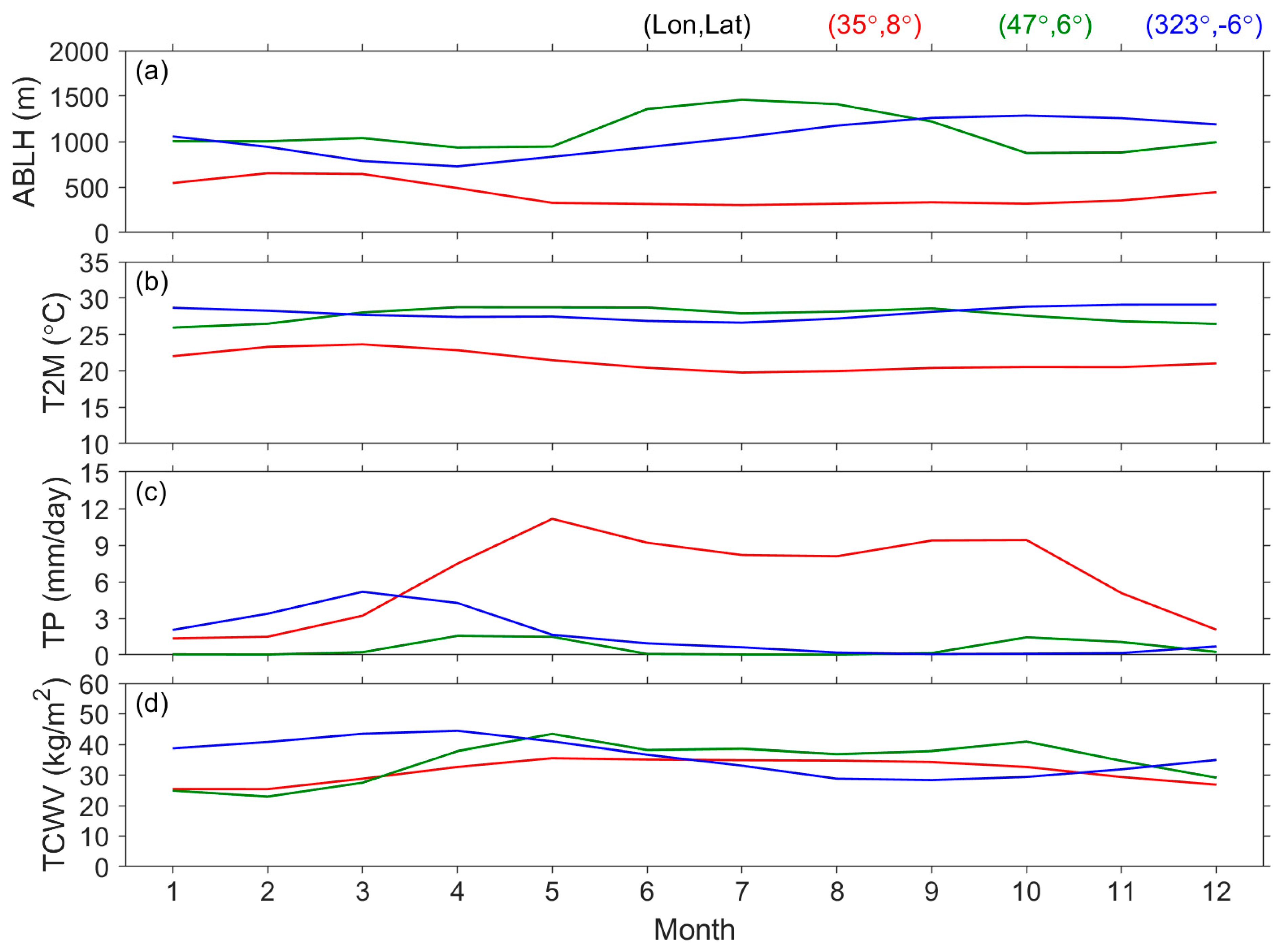
5.2. Ocean–Atmosphere Interactions

As mentioned in Section 5.1, synoptic-scale factors explain the low ABLH over the equatorial oceans and the high ABLH over the mid-latitude oceans. There are still five regions with a high ABLH over the low-latitude oceans, as enclosed by the solid lines shown in Figure 15. However, the cause of these high-ABLH regions cannot be explained by the same mechanism as discussed in Section 5.1.2 because these regions are usually occupied by semi-permanent highs during the winter months [2,61], though the stable environment within highs favors the evolution and maintenance of the ABL [1,2,3]. Since the formation of the ABL relies on interactions between the air and the surface, we turn to the surface, i.e., the ocean, to find out the causality.

5.2.1. Ocean Currents

A common point of the five high-ABLH regions (enclosed by solid lines in Figure 15) is that they are all located beside the western margins of continents. The atmospheric wind currents can drive surface ocean currents. With the effect of the Coriolis force, the large-scale surface ocean currents rotate clockwise over the northern hemispheric oceans and counter-clockwise over the southern hemispheric oceans, respectively. As a result, cold ocean currents transport cold water equatorward along the western margins of continents. In Figure 15, the cold currents that pass around the five high-ABLH regions are the California Current in the Northeast Pacific Ocean off North America, the Peru Current (also known as the Humboldt Current) in the Southeast Pacific Ocean off South America, the Canary Current in the Northeast Atlantic Ocean off North Africa, the Benguela Current in the Southeast Atlantic Ocean off Southern Africa, and the West Australian Current in the South Indian Ocean, respectively.
Over the paths of these cold currents, the air temperature, humidity, and precipitation are lower, though the cloud cover is higher than other oceanic areas at the same latitude. The lower atmosphere over these regions is further occupied by the semipermanent subtropical highs [61]. The stable weather conditions favor the evolution of the ABL, resulting in a relatively high ABLH over oceans where the cold currents flow through.
Figure 16 shows the climatology of the ABLH and meteorological parameters at (110°, −30°), (270°, −25°), and (215°, 30°), demonstrating the conditions around the West Australian, the Peru, and the California Currents, respectively. As shown in the figure, the seasonal variabilities of the T2M, TP, and TCWV are relatively small at all three places. The steady (in time) weather condition results in an ABL with an almost fixed top height. However, the ABLH is slightly higher in winter than in summer. In addition, the T2M is reasonably higher in summer than in winter due to the change in radiative heating, and the TP is slightly higher in autumn and winter than in spring and summer due to the influence of winter storms. Since the TP is relatively low at the three places, the variation in the TCWV is mainly controlled by the air temperature. These features contribute to a weak to moderate negative correlation between the ABLH and the T2M (Figure 9) and a moderate to strong negative correlation between the ABLH and the TCWV (Figure 11) over the regions influenced by cold ocean currents. Nevertheless, the correlation between the ABLH and the TP varies with place (Figure 10). For places with higher latitudes within these regions around cold ocean currents, the precipitation is more concentrated in the winter months, resulting in good consistency between the ABLH and the TP. By contrast, for places with lower latitudes within these regions, the maximum TP tends to occur earlier in autumn. The seasonal variations in the ABLH and TP are usually out of phase with a phase difference of a few months, resulting in a weak correlation between the two parameters.
However, we have to clarify some facts before ending this subsection. As mentioned in the previous paragraph, the ABLH shows negative and positive correlations with the T2M and TP, respectively, at some places within these regions around cold ocean currents. This conflicts with the mechanism introduced in Section 1, in which the evolution and maintenance of the ABL rely on fair-weather conditions. In fact, the temporal analyses and comparison, as shown in Figure 9, Figure 10, Figure 11 and Figure 16, can only describe the degree of consistency between the ABLH and each meteorological parameter. The results of the correlation analyses somewhat lack causality over the regions around cold ocean currents.

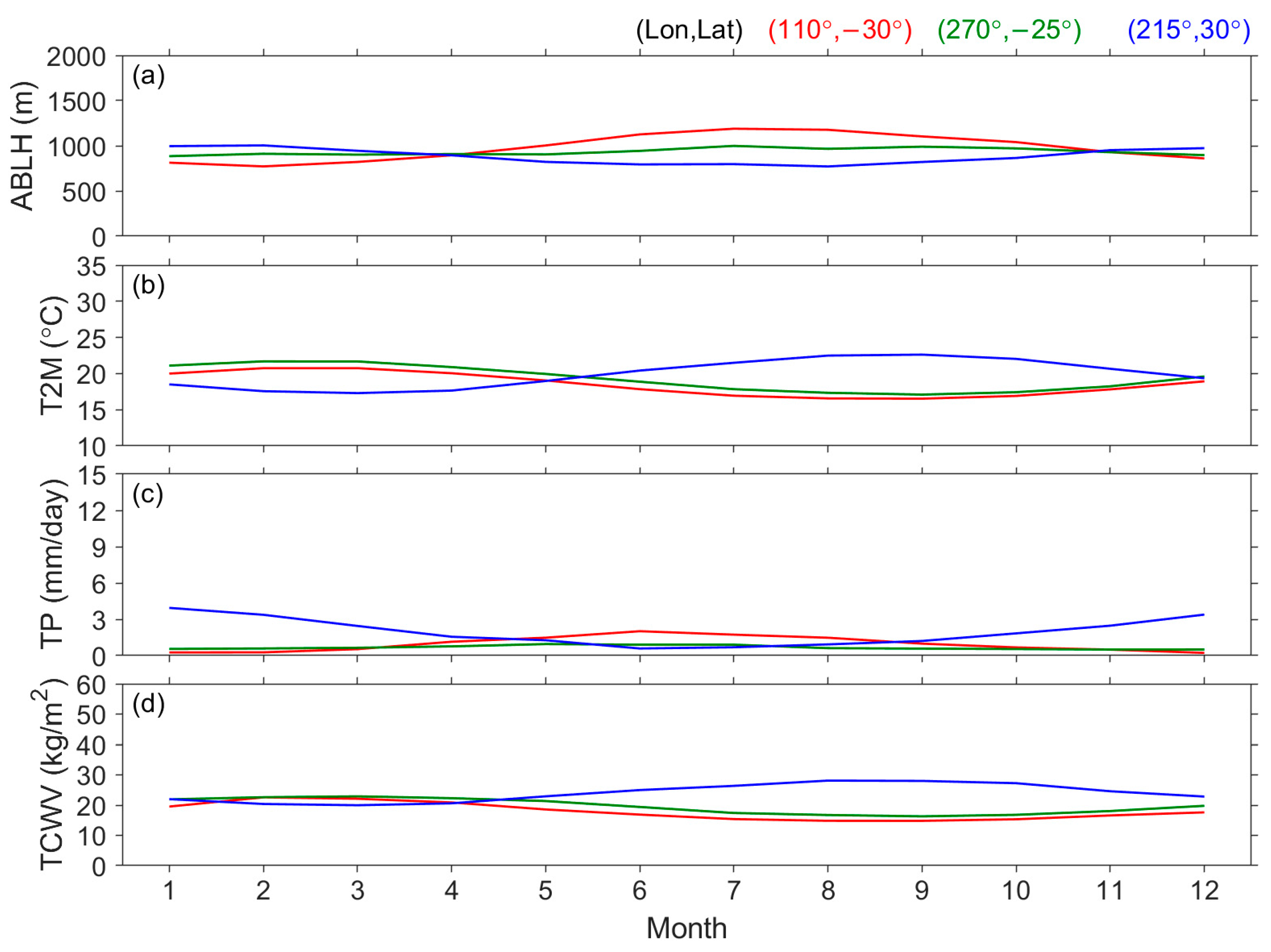
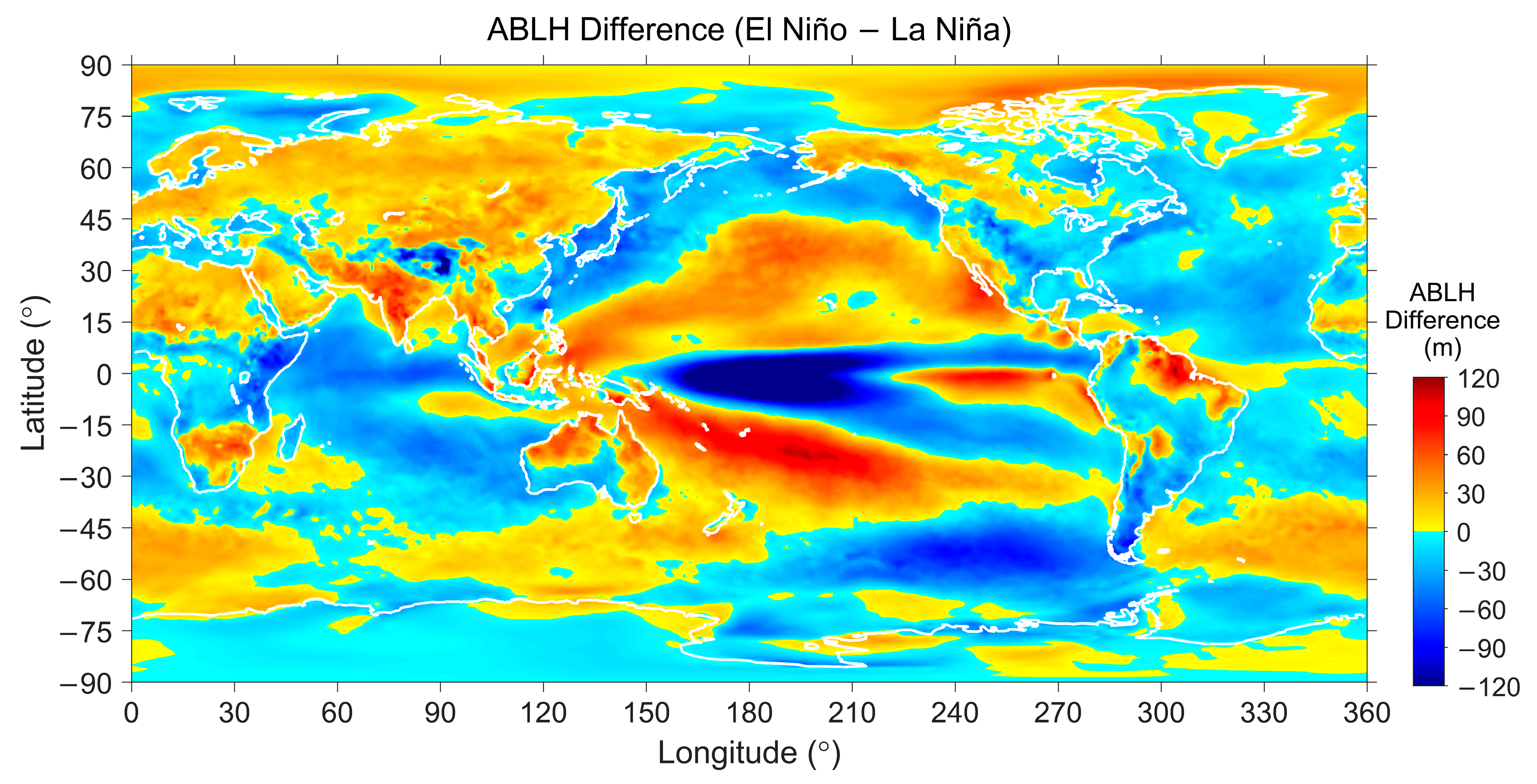
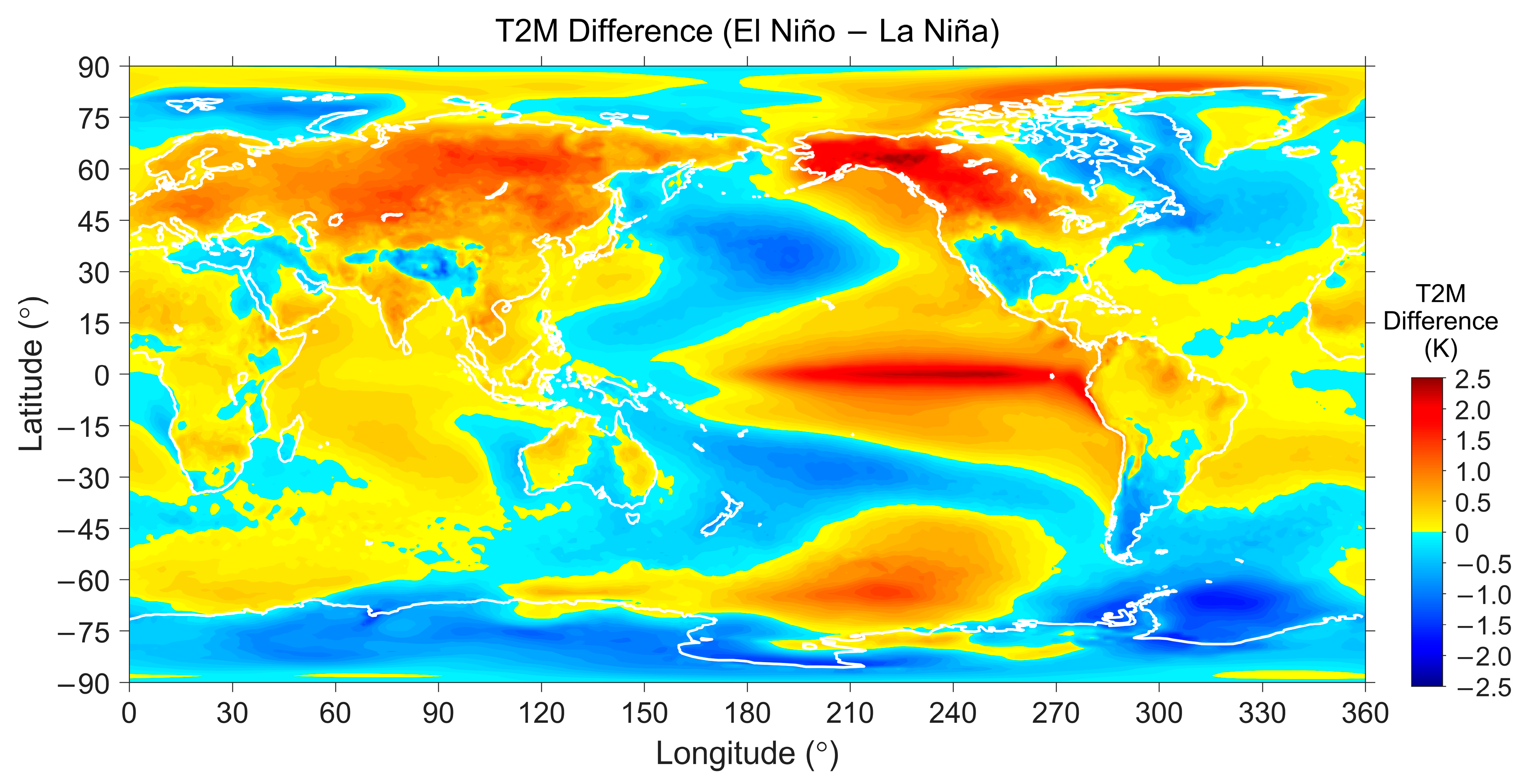
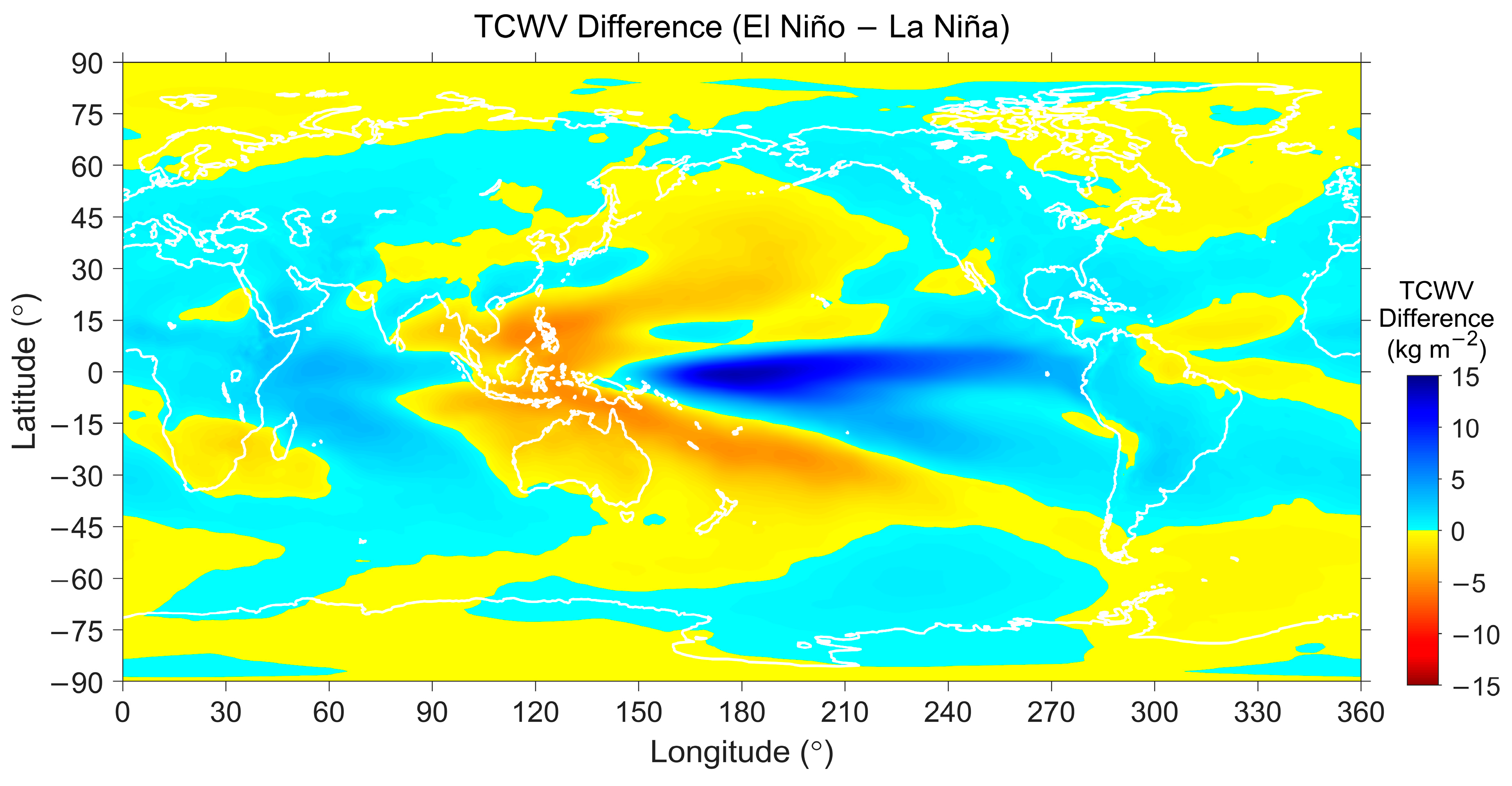
5.2.2. ABLH Response to El Niño/La Niña Events

Since the El Niño–Southern Oscillation (ENSO) is the most important ocean–atmosphere interaction phenomenon that affects the global climate, and as we are trying to discuss the possible link between the ocean and the ABLH, the response of the ABLH to El Niño/La Niña events shall also be taken up.
In the present study, we employed the Oceanic Niño Index (ONI), which is the 3-month running mean of the SST anomalies in the Niño 3.4 region, issued by the Climate Prediction Center, National Oceanic and Atmospheric Administration [62]. The El Niño (warm)/La Niña (cold) conditions are defined by the threshold of ±0.5 °C for the ONI for at least five consecutive overlapping values.
The mean ABLHs among all the El Niño and La Niña months are calculated using the same method mentioned in Section 3.1. The seasonal effects are reduced, and the response to El Niño/La Niña is enhanced after the calculation. Then, the mean ABLH of the El Niño months subtracted by the mean ABLH of the La Niña months to emphasize the difference between El Niño and La Niña conditions (abbreviated as ABLH_Diff hereafter). The result over the globe is shown in Figure 17. In addition, the differences in the mean T2M, mean TP, and mean TCWV between El Niño and La Niña conditions (abbreviated as T2M_Diff, TP_Diff, and TCWV_Diff hereafter) are also calculated using the same method. Their global distributions are plotted in Figure 18, Figure 19 and Figure 20, respectively.
In Figure 17, the positive/negative values represent that the ABLH is higher/lower during El Niño months than La Niña months. The most significant change in the ABLH, with a magnitude of about 220 m, appears over the equatorial Pacific Ocean, especially in the regions where the Pacific ITCZ and SPCZ exist (Figure 12). The Walker Circulation over the tropical Pacific Ocean is an important planetary scale circulation in the troposphere. Convection and precipitation are active near the upwelling of the Walker Circulation. The upwelling is located around 120° longitude under neutral (non-El Niño and also non-La Niña) and La Niña conditions, but it moves to around 210° longitude under El Niño conditions [2,61]. The result in Figure 17 reveals that the ABLH is lower around the upwelling of the Walker Circulation under both El Niño and La Niña conditions.
Moreover, the convergence zones also shift during El Niño events. The SPCZ shifts northeastward obviously under El Niño conditions [55,56,63], resulting in the long tail of negative values in Figure 17 extending southeastward from the position of the Walker Circulation to the coast of South America, which is accompanied by another tail of positive values on the southwestern side of it. The Pacific ICTZ also shifts about 2–5° southward, as seen from precipitation data [54,64], resulting in the narrow belt of negative values over the equatorial Pacific Ocean. Similar to the SPCZ, the SIOCZ also moves northeastward [59], lowering the ABLH over the equatorial region of Africa under El Niño conditions. No study certainly reports the migration of the SACZ due to El Niño/La Niña. However, it is known that the SACZ tends to intensify and the precipitation is higher in the southeast of South America under El Niño conditions [57,58,65]. The ABLH shows a negative deviation not only over the southeast of South America but also the southwest of South America under El Niño conditions.
On the other hand, the paths of Pacific winter storms tend to migrate noticeably southward/northward under El Niño/La Niña conditions due to the intensity and position of the blocking high in the Northern Pacific Ocean [2]. Since the ABLH is higher along the paths of winter storms (Figure 12), this migration of winter storms explains the positive and negative deviations of the ABLH over the Northern Pacific Ocean between El Niño and La Niña conditions.
The spatial correlation analysis, as performed in Section 4.3, was used to examine the spatial correlations between the ABLH_Diff and the three parameters of the T2M_Diff, TP_Diff, and TCWV_Diff. The results are summarized in Table 2.
Over lands, the ABLH_Diff and T2M_Diff have moderate to strong positive correlations in all the latitudinal sections. As seen in Figure 18, the T2M is enhanced over most land areas under El Niño conditions, though the figure cannot provide any information on the warming mechanism. The warming somehow increases the ABLH in many land areas (Figure 17), especially in the areas where the TP is reduced (Figure 19) under El Niño conditions. El Niño’s warm and dry in some continental regions, including the Indian subcontinent, the Maritime Continent, North Australia, Southern Africa (due to the migration of SIOCZ), and the northernmost of South America (Figure 19 and Figure 20). Over these regions, the weather conditions are relatively good and favor the evolution of the ABL, and the ascension of the ABLH is much more evident than in other continental areas under El Niño conditions (Figure 17).
However, over waters, the results of the correlation analysis between the ABLH_Diff and the T2M_Diff are inconsistent, and both positive and negative correlations are found in different latitudinal sections. Under El Niño conditions, the T2M is enhanced around the equatorial Pacific Ocean and the western margin of the Americas. Further, the T2M over the southernmost Pacific Ocean, the Indian Ocean, and the subtropical Atlantic Ocean is enhanced simultaneously (also refer to [66]). The ABLH (Figure 17) becomes lower over these water regions with positive deviations of the T2M (Figure 18) under El Niño conditions. Moreover, the TCWV is enhanced, but the TP is either enhanced or reduced in these regions. It seems the enhancement of the T2M (in fact, the warming of the SST) increases the cloud cover and the water vapor in the air, causing bad weather conditions and lowering the ABLH here. Therefore, the ABLH_Diff and T2M_Diff show weak to strong negative correlations over most water regions within ±60° latitude, as a correlation coefficient is given in each latitudinal section in Table 2. An exception is the southern equatorial waters, and no statistical correlation is found because the ABLH_Diff and T2M_Diff show positive correlations over the southeastern part of the equatorial Pacific Ocean (the area shown is the positive ABLH_Diff around the coast of Peru), whereas the two parameters show negative correlations over other southern equatorial waters. The former place, also famous for the etymon of El Niño, is warmer (due to the high SST; Figure 18) and dryer (Figure 19 and Figure 20) under El Niño conditions. Fair-weather conditions favor the evolution of the ABL here, resulting in the positive correlation between the ABLH_Diff and the T2M_Diff here.
In addition, the T2M_Diff shows mixed results over high-latitude waters (Figure 18). Nevertheless, the ABLH_Diff and T2M Diff are positively correlated over high-latitude waters. A higher temperature will favor the evolution of the ABL, as the ABLH and T2M are strongly positively correlated over high-latitude waters (Table 1).
On the other hand, the ABLH_Diff is negatively correlated to the TP_Diff and TCWV_Diff on the global scale. Especially, moderate to strong negative correlations are generally found over lands and waters between −60° and 10° latitudes. The ABLH varies with the changes in the TP and TCWV under El Niño/La Niña conditions, and it again follows the basic concept that bad weather restrains the vertical development of the ABL. Moreover, since the ENSO is a phenomenon sourced from the equatorial region, all three parameters of the T2M_Diff, TP_Diff, and TCWV_Diff show stronger (either positive or negative) correlation with the ABLH_Diff over here.

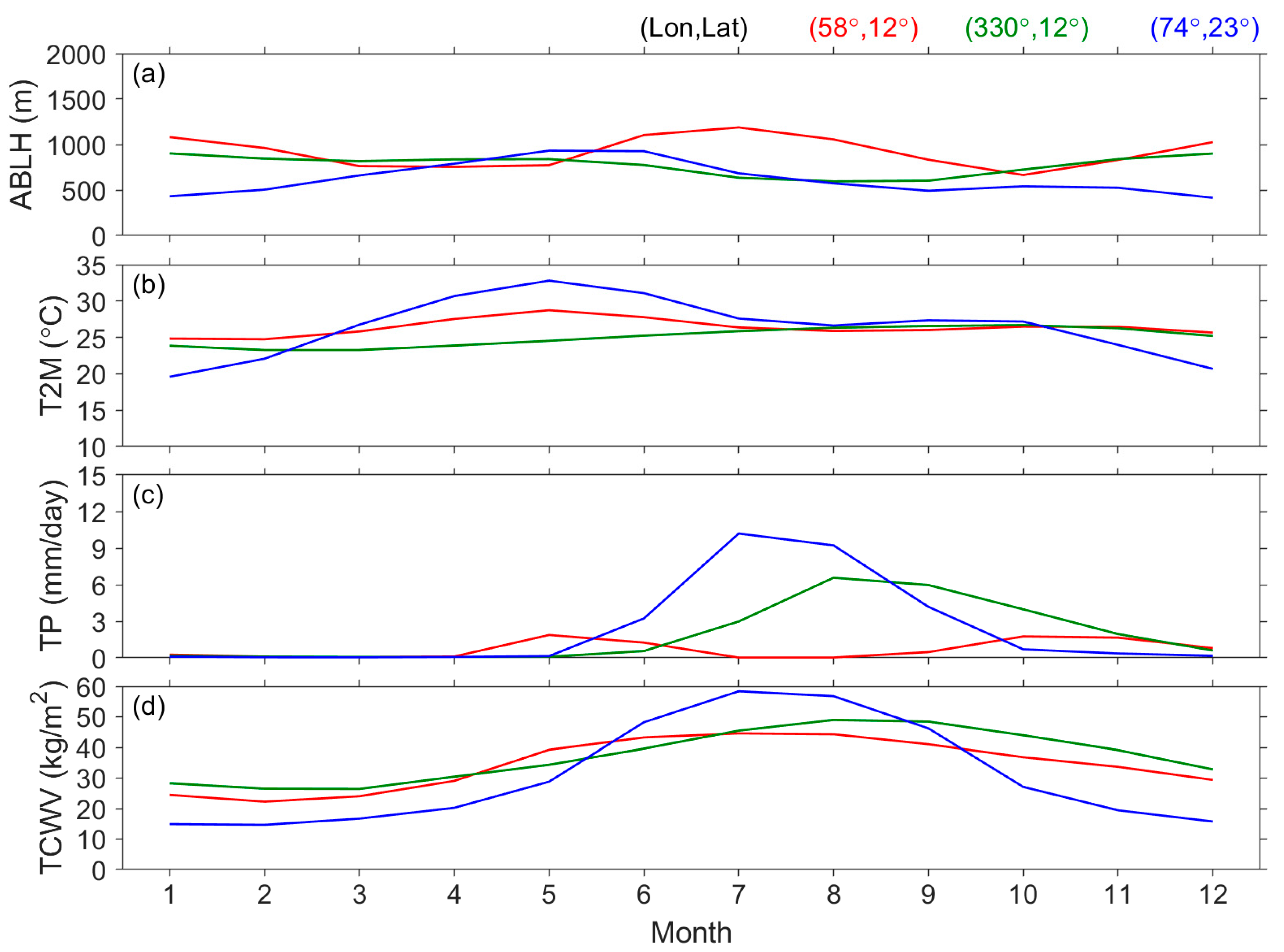
5.3. Topographic Effects

We found that the ABLH along the western margins of mountains in Central Asia (including the Altai, Tian Shan, Pamir, Himalayas, and numerous minor mountain ranges; notice that the Tibetan Plateau is not included) is very low compared with other places over continents. To find out the possible link between the terrain and the ABLH, Figure 21 again maps the mean ABLH over the globe but with topographic information overlaid. Elevation data from the GEBCO_2022 global terrain model [67] were used, and terrains with more than 1000 m elevation above sea level (ASL) are enclosed by magenta contours in the figure. Although GEBCO_2022 is a bathymetric dataset, it provides elevation data over lands. The original spatial resolution of the dataset is 15 arc-seconds, but we averaged and re-gridded the data on 1° to fit with the ABLH results.
As seen in Figure 21, the above-mentioned low-ABLH area coincides with the western margins of the Central Asia mountains, revealing the relationship between the terrain and the ABLH. In contrast, the mean ABLH is higher in the highlands in western China than in eastern China. The mean ABLH is highest in the Tibetan Plateau among all the lands. This kind of pattern, i.e., a low ABLH at the margins of mountains and a high ABLH within highlands, is also found in many mountain areas over the globe, such as the Caucasus Mountains and Iranian Plateau, the western margin of Southern Africa, and the western coast of Americas (i.e., the American Cordillera, including the mountains of Andes, Rocky, Sierra Nevada, and numerous minor mountain ranges). An opposite case is seen in the easternmost part of Africa, also known as the Horn of Africa, and here, the ABLH is lower in the mountain area but higher in the low-elevation and plain areas. We first investigate the mechanism of the low ABLH at the margins of mountains here, and the opposite case will be discussed in Section 5.4.
Figure 22 plots the climatology of the ABLH and meteorological parameters at (75°, 33°), (83°, 33°), and (252°, 33°). The first place is located at the western margins of the Himalayas, whereas the second and third places are located within the highlands of the Tibetan Plateau and Black Range, respectively. Since the elevations at the three places are pretty different, the T2M in Figure 22b uses a different numerical scale than the other figures. Among these three places, the ABLH is lowest at (75°, 33°) and highest at (83°, 33°). However, the T2M is highest at (75°, 33°) and lowest at (83°, 33°). Notice that we are trying to determine the mechanism that causes the local anomalies in the ABLH. The temperature is not the main factor controlling the local distribution of the ABLH around mountains; though, at each place, the ABLH and T2M have the same tendency in seasonal variation, as shown in Figure 22a,b.
Nevertheless, the TP and TCWV show strong negative correlations with the ABLH in both space and time. The TP and TCWV are highest at (75°, 33°) and lowest at (83°, 33°), corresponding to the lowest ABLH at (75°, 33°) and highest ABLH at (83°, 33°), respectively. Moreover, the ABLH tends to be lower in the boreal summer months, when the TP and TCWV are higher. These results are reasonable because bad weather restrains the vertical development of the ABL. Furthermore, it can hint at how the topography affects the ABLH.
The place (75°, 33°) is located on the windward side of the Himalayas, and it receives rainfall caused by the southwesterly monsoon from June to September [2,61,68], as the TP and TCWV increase during this period shown in Figure 22. The cloud cover and precipitation are expected to be more on the windward side than the lee side of mountains. Among those low-ABLH areas around mountains indicated in Figure 21, the zonal component of the near-surface wind is dominated by westerly (known by checking the 10 m u-component of the wind retrieved from ERA5). Therefore, all these areas are located on the windward side of mountains. The orographic precipitation could be the unfavorable factor that restrains the evolution of the ABL, causing a low ABLH, as seen here. By contrast, within highlands in mountain areas, such as at (83°, 33°) in the Tibetan Plateau and (252°, 33°) in the Black Range, the TP and TCWV are relatively low compared with neighboring areas because most water vapor in the air depletes around the windward side of mountains. The weather conditions are fair for favoring the evolution of the ABL, resulting in a high ABLH within highlands.

5.4. Desert and Hot Semi-Arid Climates

In Section 5.3, we mentioned an unusual case in the Horn of Africa, in which the ABLH is lower over mountain areas (the Ethiopian and Kenya highlands in Figure 21) but higher over plain areas (the area east to Ethiopian and Kenya highlands). Figure 23 plots the climatology of the ABLH and meteorological parameters at (35°, 8°) and (47°, 6°), representing the conditions in the mountain and plain areas in the Horn of Africa. As seen in the figure, the T2M is higher at (47°, 6°) than at (35°, 8°), explaining why the ABLH is also higher at (47°, 6°) than at (35°, 8°) to some degree. However, the seasonal variation in the ABLH cannot be explicated because the T2M is almost constant throughout the year. Again, bad weather plays a crucial role in the ABLH as the ABLH and TP have opposite tendencies in time.
In equatorial Africa, the moisture mainly comes from the west (the Atlantic Ocean), and the Congo Basin receives much rainfall from the west. However, as the moisture goes deep into the eastern part of equatorial Africa, the mountains along the Great Rift Valley, including the Ethiopian and Kenya highlands, restrain the eastward propagation of moisture. A low ABLH with high TP is found over the Ethiopian and Kenya highlands (Figure 6 and Figure 21). By contrast, the plain area at the easternmost of the Horn receives little rainfall, and a high ABLH with low TP is found here. This pattern is very different from other areas in which a high ABLH is found within highlands and a low ABLH is found over plains, as mentioned in Section 5.3. Nevertheless, the spatial variation in the ABLH can still be explained by the distribution of the precipitation, and the ABLH and TP show moderate to strong negative correlation here (Figure 10). Furthermore, at (35°, 8°), the TP is higher during the boreal summer and autumn months, when the ITCZ passes here, and the ABLH becomes lower during these months. By contrast, there is almost no precipitation at (47°, 6°) from June to September, and the ABLH reaches its highest level in a year (Figure 23).
A similar case can be found in the easternmost of South America. As an example in this area, the monthly means of the ABLH and meteorological parameters at (323°, −6°) are also plotted in Figure 23. The ITCZ passes between the Caribbean Sea and the northern coast of South America, and the SACZ is a crucial component contributing to the South American Monsoon system (SAMS) [69], causing abundant precipitation in the Amazon Basin. However, both the ITCZ and the SACZ miss the easternmost part of South America, and the TP is relatively low here. As a result, the ABLH is higher at this place than the neighbors, especially during the dry season in the austral winter months.

5.5. Monsoon and Seasonal Precipitation

At the high-ABLH areas in the Horn of Africa and easternmost South America, as discussed in Section 5.4, the TP has seasonal variations, as seen in Figure 23. These two places are partially influenced by the Indian [68] and South America [69] monsoon systems, which can intensively affect the precipitation in the Indian subcontinent and South America, respectively.
A small area with a high ABLH exists in the North India Ocean and between the Horn of Africa and the Indian subcontinent. The ABLH within this area is about 800–1100 m, whereas the ABLH is usually about 600–900 m in northern low-latitude waters (Figure 4). We have to check the meteorological parameters to know why the ABLH is higher in this area, though it is a local phenomenon and negligible compared to the global distribution of the ABLH.
Figure 24 shows the climatology of the ABLH and meteorological parameters at (58°, 12°) to the northeast of the Horn of Africa. The values at (330°, 12°) are also plotted for reference. We first look at (330°, 12°) to know the general climatology in the northern low-latitude waters. The ITCZ migrates to the northern low latitudes with precipitations during the boreal summer months. At (330°, 12°), the TP is approximately zero from January to May, but it increases to a maximum of about 6 mm/day in August due to the influence of the ITCZ, further causing an evident seasonal variation in the TP. The ABLH at this place, expectedly, has a similar seasonal variation but the opposite tendency. The ABLH is usually higher in the boreal winter and spring months but becomes lower when the TP increases during the influence of the ITCZ.
Then, we turn back to (58°, 12°). This place has a similar climatology of the T2M and even the TCWV as at (330°, 12°). However, there is almost no rain from June to September, when the Indian monsoon influences the North Indian Ocean and the Indian subcontinent [68]. The monsoon brings southwesterly and northeasterly winds during the boreal summer and winter months, respectively. During the southwesterly monsoon, winds from Mascarene high in the South Indian Ocean flow across the equator, becoming southwesterly due to the Coriolis force in the North Indian Ocean. Moisture from the southern hemisphere is thus transported to the Indian subcontinent. Although the TCWV along the transportation path is high, no terrain restrains the moisture transportation over the waters, and the TP is relatively low in the northwestern part of the Indian Ocean. In such a situation, the evolution of the ABL is favored by the thermal and wet flows, resulting in a higher ABLH during the southwesterly monsoon season, as seen in Figure 24a.
One more thing is worth mentioning here. The plain area in the Horn of Africa, as discussed in Section 5.4, is also affected by monsoon systems [68,70]. Multiple meteorological processes play crucial roles in modifying the moisture flows and precipitation in East Africa, the North Indian Ocean, and the Indian subcontinent. As a result, the precipitation and the ABLH climatology in this plain area (i.e., (47°, 6°) in Figure 23) are quite similar to those in the water area ((58°, 12°) in Figure 24) to the northeast of it, though the former is at land and the latter is at sea, respectively.
At last, we look at the Indian subcontinent to see how the Indian monsoon affects the ABLH in this area. The annual cycle at (74°, 23°) is plotted in Figure 24 as well, though the mean ABLH at this place is not the lowest in the Indian subcontinent. A large area in the subcontinent is occupied by the Deccan Plateau, but the place of (74°, 23°) is located in the drainage basin of the Sabarmati River, enabling us to understand the effect of monsoon on the ABLH without topographic effects. The TP at (74°, 23°) is approximately zero from October to May in the next year, but it increases dramatically during the southwesterly monsoon season from June to September. The T2M, in general, shall increase during summer, but it maximizes in May and then decreases due to the bad weather caused by monsoon. The monthly ABLH thus descends during the summer months. Although the climatology of the ABLH at (74°, 23°) is very different from the normal condition, as shown in Figure 4e, the temporal variation in the ABLH at this place influenced by monsoon can still be explained by the same mechanisms that we have repeated many times in this study. During the winter months, the Indian subcontinent is affected by the northeasterly monsoon, fair-weather conditions with relatively low moisture favor the evolution of the ABL, and the ABLH is generally positively correlated to the T2M, i.e., the ABL top ascends as the T2M increases in spring months. The process works well until the southwesterly monsoon onsets in June. The southwesterly monsoon brings much moisture, causing intensive precipitation from June to September. Further, the bad weather restrains the evolution of the ABL, lowering the ABL top and resulting in a much different climatology of the ABLH.

6. Summary and Conclusions

The atmospheric boundary layer (ABL), as the bottommost layer of the atmosphere, affects the hydrological cycle, energy exchange, and particle transportation in the troposphere. Geophysical processes within the ABL influence the temperature and wind, playing crucial roles in the weather and climate [1,2,3]. Meanwhile, the performance of weather and climate models highly relies on the representation of the ABL [5].
The morphology of the ABLH, either globally or in a local area, has been studied using many different datasets and methods in the literature, as introduced in Section 1. However, a correlation study between the ABLH and meteorology, as well as a discussion on the controlling factors of the ABLH from the global to local scale, are absent from the literature.
In the present study, the ABL height (ABLH) retrieved from the ERA5 reanalysis dataset was used to investigate the spatio-temporal variation, i.e., climatology of the ABLH, and 45 years of data from 1979 to 2023 were used. As reanalysis retrievals of the ABLH have been compared and further validated with other datasets (e.g., [19,21,43,46]), this study does not focus on the comparison between our results and other papers but pays attention to explaining the mechanisms, i.e., controlling factors, that affect the ABLH. The results and discussions in this study are divided into three parts: general climatology in Section 3, correlation analyses in Section 4, and controlling factors in the spatio-temporal variations in the ABLH in Section 5, respectively.
In Section 3, the global 45-year mean ABLH (Figure 1) shows an apparent difference between lands and waters. In general, the mean ABLH is higher over waters than lands. However, the temporal variability (standard deviation) of the ABLH is higher over lands than waters (Figure 2). The diurnal variation in the ABLH is significant over lands but negligible over waters (Figure 3). On the other hand, seasonal variations are observed over both lands and waters, with different magnitudes at different latitudes; however, the seasonal variations over lands and waters are out of phase at low and mid-latitudes (Figure 4). Antarctica is an exception in that both the diurnal and seasonal variations are negligible.
Fair weather favors, but bad weather restrains, the evolution of the ABL. Nevertheless, “fair weather” and “bad weather” are hard to define clearly. Therefore, we selected three meteorological parameters, which are the 2 m temperature (T2M), total precipitation (TP), and total column water vapor (TCWV), as proxies of the weather conditions. The spatial (Table 1) and temporal correlation analyses (Figure 9, Figure 10 and Figure 11) between the ABLH and these meteorological parameters point out some general rules. Usually, the ABLH is higher where or when the T2M is also higher (positive correlation), but the ABLH is lower where or when the TP is higher (negative correlation). However, the T2M and TP could be either both high or low at the same time. In such a situation, the TCWV is used to diagnose which parameter dominates the ABLH, and the threshold is 15 kg m−2. The ABLH is mainly dominated by the T2M under dry conditions (TCWV < 15 kg m−2) and by the TP under wet conditions (TCWV > 15 kg m−2), respectively (Figure 8), as concluded in Section 4.
Figure 3 and Figure 4 show the general properties of the ABLH from the global perspective. However, Figure 1 reveals many local features of the mean ABLH (spatial variability). Figure 2 also reveals that the ABLH is variable in some areas (temporal variability). With the conclusion drawn in Section 4, Section 5 lists several factors that may affect the spatial or temporal properties of the ABLH, including the following. (1) Synoptic weather systems: the ABLH is lower over convergence zones (Figure 12 and Figure 13) but higher along the paths of winter storms (extratropical cyclones and fronts) (Figure 12 and Figure 14). (2) Ocean–atmosphere interaction: the ABLH is higher over oceanic areas flowed through by cold currents (Figure 15 and Figure 16). On the other hand, El Niño and La Niña events can modify meteorological parameters and the pattern of weather systems, further heightening or lowering the ABLH during El Niño and La Niña events (Figure 17). (3) Topography: the ABLH is lower at the margins of mountains due to orographic precipitation but is higher in highlands of mountains due to fair weather (Figure 21 and Figure 22). (4) Desert and hot semi-arid climates: hot and dry weather conditions favor the vertical extension of the ABL, areas with desert and hot semi-arid climates have a higher ABLH (Figure 21 and Figure 23). (5) Monsoon: seasonal variations in the prevailing wind and precipitation modify the weather conditions in areas affected by monsoon, resulting in a corresponding seasonal variation in the ABLH (Figure 21 and Figure 24).
The present study investigates the climatology of the ABLH, determines the relationship between the ABLH and meteorological parameters, and summarizes several controlling factors that affect the ABLH. On the basis of the results, our next attempt will be the parameterized estimation of the ABLH. Also, since the ABL properties are involved in may atmospheric physical and chemical processes, as mentioned in Section 1, the conclusions of the present study are expected to enhance the performance of predictions in weather and climate applications, such as the boundary layer meteorology simulation, air pollutant dispersion, wind power estimation and prediction, and even bird migration.

Supplementary Materials

The following supporting information can be downloaded at: https://www.mdpi.com/article/10.3390/atmos16050573/s1, Figure S1. The mean height of atmospheric boundary layer (ABLH) above ground level (AGL) in January. Figure S2. Same as Figure S1, but showing the mean ABLH in February. Figure S3. Same as Figure S1, but showing the mean ABLH in March. Figure S4. Same as Figure S1, but showing the mean ABLH in April. Figure S5. Same as Figure S1, but showing the mean ABLH in May. Figure S6. Same as Figure S1, but showing the mean ABLH in June. Figure S7. Same as Figure S1, but showing the mean ABLH in July. Figure S8. Same as Figure S1, but showing the mean ABLH in August. Figure S9. Same as Figure S1, but showing the mean ABLH in September. Figure S10. Same as Figure S1, but showing the mean ABLH in October. Figure S11. Same as Figure S1, but showing the mean ABLH in November. Figure S12 Same as Figure S1, but showing the mean ABLH in December. Figure S13. Same as Figure S1, but showing the mean ABLH at 00LT. Figure S14. Same as Figure S1, but showing the mean ABLH at 01LT. Figure S15. Same as Figure S1, but showing the mean ABLH at 02LT. Figure S16. Same as Figure S1, but showing the mean ABLH at 03LT. Figure S17. Same as Figure S1, but showing the mean ABLH at 04LT. Figure S18. Same as Figure S1, but showing the mean ABLH at 05LT. Figure S19. Same as Figure S1, but showing the mean ABLH at 06LT. Figure S20. Same as Figure S1, but showing the mean ABLH at 07LT. Figure S21. Same as Figure S1, but showing the mean ABLH at 08LT. Figure S22. Same as Figure S1, but showing the mean ABLH at 09LT. Figure S23. Same as Figure S1, but showing the mean ABLH at 10LT. Figure S24. Same as Figure S1, but showing the mean ABLH at 11LT. Figure S25. Same as Figure S1, but showing the mean ABLH at 12LT. Figure S26. Same as Figure S1, but showing the mean ABLH at 13LT. Figure S27. Same as Figure S1, but showing the mean ABLH at 14LT. Figure S28. Same as Figure S1, but showing the mean ABLH at 15LT. Figure S29. Same as Figure S1, but showing the mean ABLH at 16LT. Figure S30. Same as Figure S1, but showing the mean ABLH at 17LT. Figure S31. Same as Figure S1, but showing the mean ABLH at 18LT. Figure S32. Same as Figure S1, but showing the mean ABLH at 19LT. Figure S33. Same as Figure S1, but showing the mean ABLH at 20LT. Figure S34. Same as Figure S1, but showing the mean ABLH at 21LT. Figure S35. Same as Figure S1, but showing the mean ABLH at 22LT. Figure S36. Same as Figure S1, but showing the mean ABLH at 23LT.

Author Contributions

Conceptualization, C.-J.P.; methodology, S.-S.Y.; validation, C.-J.P. and S.-S.Y.; formal analysis, S.-S.Y.; investigation, S.-S.Y.; resources, C.-J.P.; data curation, S.-S.Y.; writing—original draft preparation, S.-S.Y.; writing—review and editing, S.-S.Y. and C.-J.P.; supervision, C.-J.P.; project administration, C.-J.P.; funding acquisition, C.-J.P. All authors have read and agreed to the published version of the manuscript.

Funding

This research was funded by the National Science and Technology Council (former Ministry of Science and Technology) of Taiwan, grant number MOST 110-2111-M-008-009, MOST 111-2111-M-008-009, MOST 110-2811-M-008-532, and MOST 111-2811-M-008-039.

Institutional Review Board Statement

Not applicable.

Informed Consent Statement

Not applicable.

Data Availability Statement

The original data (ERA5) presented in this study are openly available in the Copernicus Climate Data Store (CDS) at https://doi.org/10.24381/cds.adbb2d47 or https://cds.climate.copernicus.eu/ (accessed on 6 January 2025) implemented by the European Centre for Medium-Range Weather Forecasts (ECMWF).

Acknowledgments

The authors thank the two anonymous reviewers and Hung-Chun Hou for their helpful comments and suggestions on this paper. The authors also thank the ECMWF, who produced the ERA5 atmospheric reanalysis dataset within the Copernicus Climate Change Service (C3S).

Conflicts of Interest

The authors declare no conflicts of interest.

Abbreviations

The following abbreviations are used in this manuscript:
ABLAtmospheric boundary layer
ABLHAtmospheric boundary layer height
PBLPlanetary boundary layer
EZEntrainment zone
CICapping inversion
MLMixed layer
SSTSea surface temperature
ECMWFEuropean Centre for Medium-Range Weather Forecasts
AGLAbove ground level
LTLocal time
UTUniversal time
T2M2 m temperature
TPTotal precipitation
TCWVTotal column water vapor
ITCZIntertropical convergence zone
SPCZSouth Pacific convergence zone
SACZSouth Atlantic convergence zone
SIOCZSouth Indian Ocean convergence zone
NWPNorthwest Pacific Ocean off Japan
NANorth Atlantic Ocean off North America
ONIOceanic Niño Index
ABLH_DiffABLH difference between El Niño and La Niña conditions
T2M_DiffT2M difference between El Niño and La Niña conditions
TP_DiffTP difference between El Niño and La Niña conditions
TCWV_DiffTCWV difference between El Niño and La Niña conditions

References

  1. Stull, R.B. An Introduction to Boundary Layer Meteorology; Kluwer Academic Publishers: Dordrecht, The Netherlands, 1988. [Google Scholar] [CrossRef]
  2. Stull, R. Practical Meteorology: An Algebra-Based Survey of Atmospheric Science; Version 1.02b ed.; University of British Columbia: Vancouver, BC, Canada, 2017. [Google Scholar]
  3. Garratt, J.R. The Atmospheric Boundary Layer; Cambridge University Press: Melbourne, Australia, 1994; p. 336. [Google Scholar]
  4. Fu, X.; Wang, B. The role of longwave radiation and boundary layer thermodynamics in forcing tropical surface winds. J. Clim. 1999, 12, 1049–1069. [Google Scholar] [CrossRef]
  5. Holtslag, A.A.M.; Svensson, G.; Baas, P.; Basu, S.; Beare, B.; Beljaars, A.C.M.; Bosveld, F.C.; Cuxart, J.; Lindvall, J.; Steeneveld, G.J.; et al. Stable atmospheric boundary layers and diurnal cycles: Challenges for weather and climate models. Bull. Am. Meteorol. Soc. 2013, 94, 1691–1706. [Google Scholar] [CrossRef]
  6. Larson, K.; Hartmann, D.L.; Klein, S.A. The role of clouds, water vapor, circulation, and boundary layer structure in the sensitivity of the tropical climate. J. Clim. 1999, 12, 2359–2374. [Google Scholar] [CrossRef]
  7. Kerlinger, P.; Moore, F.R. Atmospheric Structure and Avian Migration. In Current Ornithology; Power, D.M., Ed.; Springer: Boston, MA, USA, 1989; pp. 109–142. [Google Scholar] [CrossRef]
  8. Shannon, H.D.; Young, G.S.; Yates, M.A.; Fuller, M.R.; Seegar, W.S. Measurements of thermal updraft intensity over complex terrain using American white pelicans and a simple boundary-layer forecast model. Bound.-Layer Meteorol. 2002, 104, 167–199. [Google Scholar] [CrossRef]
  9. Mandel, J.T.; Bildstein, K.L.; Bohrer, G.; Winkler, D.W. Movement ecology of migration in turkey vultures. Proc. Natl. Acad. Sci. USA 2008, 105, 19102–19107. [Google Scholar] [CrossRef]
  10. Bott, A. A numerical model of the cloud-topped planetary boundary-layer: Impact of aerosol particles on the radiative forcing of stratiform clouds. Q. J. R. Meteorol. Soc. 1997, 123, 631–656. [Google Scholar] [CrossRef]
  11. Murphy, D.M.; Anderson, J.R.; Quinn, P.K.; McInnes, L.M.; Brechtel, F.J.; Kreidenweis, S.M.; Middlebrook, A.M.; Pósfai, M.; Thomson, D.S.; Buseck, P.R. Influence of sea-salt on aerosol radiative properties in the Southern Ocean marine boundary layer. Nature 1998, 392, 62–65. [Google Scholar] [CrossRef]
  12. Yu, H.; Liu, S.C.; Dickinson, R.E. Radiative effects of aerosols on the evolution of the atmospheric boundary layer. J. Geophys. Res. Atmos. 2002, 107, AAC 3-1–AAC 3-14. [Google Scholar] [CrossRef]
  13. Gao, Y.; Zhang, M.; Liu, Z.; Wang, L.; Wang, P.; Xia, X.; Tao, M.; Zhu, L. Modeling the feedback between aerosol and meteorological variables in the atmospheric boundary layer during a severe fog–haze event over the North China Plain. Atmos. Chem. Phys. 2015, 15, 4279–4295. [Google Scholar] [CrossRef]
  14. Petäjä, T.; Järvi, L.; Kerminen, V.M.; Ding, A.J.; Sun, J.N.; Nie, W.; Kujansuu, J.; Virkkula, A.; Yang, X.; Fu, C.B.; et al. Enhanced air pollution via aerosol-boundary layer feedback in China. Sci. Rep. 2016, 6, 18998. [Google Scholar] [CrossRef]
  15. Wood, R.; Bretherton, C.S. Boundary layer depth, entrainment, and decoupling in the cloud-capped subtropical and tropical marine boundary layer. J. Clim. 2004, 17, 3576–3588. [Google Scholar] [CrossRef]
  16. Medeiros, B.; Hall, A.; Stevens, B. What controls the mean depth of the PBL? J. Clim. 2005, 18, 3157–3172. [Google Scholar] [CrossRef]
  17. Basha, G.; Ratnam, M.V. Identification of atmospheric boundary layer height over a tropical station using high-resolution radiosonde refractivity profiles: Comparison with GPS radio occultation measurements. J. Geophys. Res. Atmos. 2009, 114, D16101. [Google Scholar] [CrossRef]
  18. Guo, P.; Kuo, Y.-H.; Sokolovskiy, S.V.; Lenschow, D.H. Estimating atmospheric boundary layer depth using COSMIC radio occultation data. J. Atmos. Sci. 2011, 68, 1703–1713. [Google Scholar] [CrossRef]
  19. Ao, C.O.; Waliser, D.E.; Chan, S.K.; Li, J.-L.; Tian, B.; Xie, F.; Mannucci, A.J. Planetary boundary layer heights from GPS radio occultation refractivity and humidity profiles. J. Geophys. Res. Atmos. 2012, 117, D16117. [Google Scholar] [CrossRef]
  20. Seidel, D.J.; Zhang, Y.; Beljaars, A.; Golaz, J.-C.; Jacobson, A.R.; Medeiros, B. Climatology of the planetary boundary layer over the continental United States and Europe. J. Geophys. Res. Atmos. 2012, 117, D17106. [Google Scholar] [CrossRef]
  21. von Engeln, A.; Teixeira, J. A planetary boundary layer height climatology derived from ECMWF reanalysis data. J. Clim. 2013, 26, 6575–6590. [Google Scholar] [CrossRef]
  22. Basha, G.; Kishore, P.; Ratnam, M.V.; Ravindra Babu, S.; Velicogna, I.; Jiang, J.H.; Ao, C.O. Global climatology of planetary boundary layer top obtained from multi-satellite GPS RO observations. Clim. Dyn. 2018, 52, 2385–2398. [Google Scholar] [CrossRef]
  23. Hooper, W.P.; Eloranta, E.W. Lidar measurements of wind in the planetary boundary layer: The method, accuracy and results from joint measurements with radiosonde and kytoon. J. Appl. Meteorol. Climatol. 1986, 25, 990–1001. [Google Scholar] [CrossRef]
  24. Sempreviva, A.M.; Gryning, S.-E. Mixing height over water and its role on the correlation between temperature and humidity fluctuations in the unstable surface layer. Bound.-Layer Meteorol. 2000, 97, 273–291. [Google Scholar] [CrossRef]
  25. Johansson, C.; Bergström, H. An auxiliary tool to determine the height of the boundary layer. Bound.-Layer Meteorol. 2005, 115, 423–432. [Google Scholar] [CrossRef]
  26. Seidel, D.J.; Ao, C.O.; Li, K. Estimating climatological planetary boundary layer heights from radiosonde observations: Comparison of methods and uncertainty analysis. J. Geophys. Res. Atmos. 2010, 115, D16113. [Google Scholar] [CrossRef]
  27. Holden, J.J.; Derbyshire, S.H.; Belcher, S.E. Tethered balloon observations of the nocturnal stable boundary layer in a valley. Bound.-Layer Meteorol. 2000, 97, 1–24. [Google Scholar] [CrossRef]
  28. Dang, R.; Yang, Y.; Hu, X.-M.; Wang, Z.; Zhang, S. A review of techniques for diagnosing the atmospheric boundary layer height (ABLH) using aerosol lidar data. Remote Sens. 2019, 11, 1590. [Google Scholar] [CrossRef]
  29. Ecklund, W.L.; Carter, D.A.; Balsley, B.B. A UHF wind profiler for the boundary layer: Brief description and initial results. J. Atmos. Ocean. Technol. 1988, 5, 432–441. [Google Scholar] [CrossRef]
  30. Rogers, R.R.; Ecklund, W.L.; Carter, D.A.; Gage, K.S.; Ethier, S.A. Research applications of a boundary-layer wind profiler. Bull. Am. Meteorol. Soc. 1993, 74, 567–580. [Google Scholar] [CrossRef]
  31. Bianco, L.; Wilczak, J.M. Convective boundary layer depth: Improved measurement by doppler radar wind profiler using fuzzy logic methods. J. Atmos. Ocean. Technol. 2002, 19, 1745–1758. [Google Scholar] [CrossRef]
  32. Helmis, C.G.; Sgouros, G.; Tombrou, M.; Schäfer, K.; Münkel, C.; Bossioli, E.; Dandou, A. A comparative study and evaluation of mixing-height estimation based on sodar-RASS, ceilometer data and numerical model simulations. Bound.-Layer Meteorol. 2012, 145, 507–526. [Google Scholar] [CrossRef]
  33. Cimini, D.; De Angelis, F.; Dupont, J.C.; Pal, S.; Haeffelin, M. Mixing layer height retrievals by multichannel microwave radiometer observations. Atmos. Meas. Tech. 2013, 6, 2941–2951. [Google Scholar] [CrossRef]
  34. Saeed, U.; Rocadenbosch, F.; Crewell, S. Synergetic use of LiDAR and microwave radiometer observations for boundary-layer height detection. In Proceedings of the 2015 IEEE International Geoscience and Remote Sensing Symposium (IGARSS), Milan, Italy, 26–31 July 2015; pp. 3945–3948. [Google Scholar]
  35. Smedman, A.-S.; Tjernström, M.; Högström, U. The near-neutral marine atmospheric boundary layer with no surface shearing stress: A case study. J. Atmos. Sci. 1994, 51, 3399–3411. [Google Scholar] [CrossRef]
  36. Smedman, A.; Högström, U.; Bergström, H.; Rutgersson, A.; Kahma, K.K.; Pettersson, H. A case study of air-sea interaction during swell conditions. J. Geophys. Res. Ocean. 1999, 104, 25833–25851. [Google Scholar] [CrossRef]
  37. Gryning, S.-E.; Batchvarova, E. Marine boundary layer and turbulent fluxes over the Baltic Sea: Measurements and modelling. Bound.-Layer Meteorol. 2002, 103, 29–47. [Google Scholar] [CrossRef]
  38. McGrath-Spangler, E.L.; Denning, A.S. Global seasonal variations of midday planetary boundary layer depth from CALIPSO space-borne LIDAR. J. Geophys. Res. Atmos. 2013, 118, 1226–1233. [Google Scholar] [CrossRef]
  39. Fetzer, E.J.; Teixeira, J.; Olsen, E.T.; Fishbein, E.F. Satellite remote sounding of atmospheric boundary layer temperature inversions over the subtropical eastern Pacific. Geophys. Res. Lett. 2004, 31, L17102. [Google Scholar] [CrossRef]
  40. Martins, J.P.A.; Teixeira, J.; Soares, P.M.M.; Miranda, P.M.A.; Kahn, B.H.; Dang, V.T.; Irion, F.W.; Fetzer, E.J.; Fishbein, E. Infrared sounding of the trade-wind boundary layer: AIRS and the RICO experiment. Geophys. Res. Lett. 2010, 37, L24806. [Google Scholar] [CrossRef]
  41. von Engeln, A.; Teixeira, J.; Wickert, J.; Buehler, S.A. Using CHAMP radio occultation data to determine the top altitude of the Planetary Boundary Layer. Geophys. Res. Lett. 2005, 32, L06815. [Google Scholar] [CrossRef]
  42. Sokolovskiy, S.; Kuo, Y.-H.; Rocken, C.; Schreiner, W.S.; Hunt, D.; Anthes, R.A. Monitoring the atmospheric boundary layer by GPS radio occultation signals recorded in the open-loop mode. Geophys. Res. Lett. 2006, 33, L12813. [Google Scholar] [CrossRef]
  43. Guo, J.; Miao, Y.; Zhang, Y.; Liu, H.; Li, Z.; Zhang, W.; He, J.; Lou, M.; Yan, Y.; Bian, L.; et al. The climatology of planetary boundary layer height in China derived from radiosonde and reanalysis data. Atmos. Chem. Phys. 2016, 16, 13309–13319. [Google Scholar] [CrossRef]
  44. Berrisford, P.; Dee, D.; Poli, P.; Brugge, R.v.d.; Fielding, K.; Fuentes, M.; Kållberg, P.W.; Kobayashi, S.; Uppala, S.M.; Simmons, A.H. The ERA-Interim Archive, Version 2.0; European Centre for Medium Range Weather Forecasts: Reading, UK, 2011. [Google Scholar]
  45. Complete ERA5 from 1979: Fifth Generation of ECMWF Atmospheric Reanalyses of the Global Climate. Available online: https://doi.org/10.24381/cds.adbb2d47 (accessed on 6 January 2025).
  46. Guo, J.; Zhang, J.; Yang, K.; Liao, H.; Zhang, S.; Huang, K.; Lv, Y.; Shao, J.; Yu, T.; Tong, B.; et al. Investigation of near-global daytime boundary layer height using high-resolution radiosondes: First results and comparison with ERA5, MERRA-2, JRA-55, and NCEP-2 reanalyses. Atmos. Chem. Phys. 2021, 21, 17079–17097. [Google Scholar] [CrossRef]
  47. Dias-Júnior, C.Q.; Carneiro, R.G.; Fisch, G.; D’Oliveira, F.A.F.; Sörgel, M.; Botía, S.; Machado, L.A.T.; Wolff, S.; Santos, R.M.N.d.; Pöhlker, C. Intercomparison of planetary boundary layer heights using remote sensing retrievals and ERA5 reanalysis over central Amazonia. Remote Sens. 2022, 14, 4561. [Google Scholar] [CrossRef]
  48. Saha, S.; Sharma, S.; Kumar, K.N.; Kumar, P.; Lal, S.; Kamat, D. Investigation of atmospheric boundary layer characteristics using ceilometer lidar, COSMIC GPS RO satellite, radiosonde and ERA-5 reanalysis dataset over western Indian region. Atmos. Res. 2022, 268, 105999. [Google Scholar] [CrossRef]
  49. Sinclair, V.A.; Ritvanen, J.; Urbancic, G.; Statnaia, I.; Batrak, Y.; Moisseev, D.; Kurppa, M. Boundary-layer height and surface stability at Hyytiälä, Finland, in ERA5 and observations. Atmos. Meas. Tech. 2022, 15, 3075–3103. [Google Scholar] [CrossRef]
  50. Slättberg, N.; Lai, H.-W.; Chen, X.; Ma, Y.; Chen, D. Spatial and temporal patterns of planetary boundary layer height during 1979–2018 over the Tibetan Plateau using ERA5. Int. J. Climatol. 2022, 42, 3360–3377. [Google Scholar] [CrossRef]
  51. Hersbach, H.; Bell, B.; Berrisford, P.; Hirahara, S.; Horányi, A.; Muñoz-Sabater, J.; Nicolas, J.; Peubey, C.; Radu, R.; Schepers, D.; et al. The ERA5 global reanalysis. Q. J. R. Meteorol. Soc. 2020, 146, 1999–2049. [Google Scholar] [CrossRef]
  52. ECMWF. IFS Documentation CY41R2—Part IV: Physical Processes. In IFS Documentation CY41R2; ECMWF: Reading, UK, 2016. [Google Scholar] [CrossRef]
  53. ECMWF. ERA5: Data Documentation. Available online: https://confluence.ecmwf.int/pages/viewpage.action?pageId=76414402 (accessed on 12 December 2022).
  54. Schneider, T.; Bischoff, T.; Haug, G.H. Migrations and dynamics of the intertropical convergence zone. Nature 2014, 513, 45–53. [Google Scholar] [CrossRef]
  55. Vincent, D.G. The South Pacific convergence zone (SPCZ): A review. Mon. Weather. Rev. 1994, 122, 1949–1970. [Google Scholar] [CrossRef]
  56. Brown, J.R.; Lengaigne, M.; Lintner, B.R.; Widlansky, M.J.; van der Wiel, K.; Dutheil, C.; Linsley, B.K.; Matthews, A.J.; Renwick, J. South Pacific Convergence Zone dynamics, variability and impacts in a changing climate. Nat. Rev. Earth Environ. 2020, 1, 530–543. [Google Scholar] [CrossRef]
  57. Carvalho, L.M.V.; Jones, C.; Liebmann, B. Extreme precipitation events in southeastern south America and large-scale convective patterns in the South Atlantic convergence zone. J. Clim. 2002, 15, 2377–2394. [Google Scholar] [CrossRef]
  58. Carvalho, L.M.V.; Jones, C.; Liebmann, B. The South Atlantic convergence zone: Intensity, form, persistence, and relationships with intraseasonal to interannual activity and extreme rainfall. J. Clim. 2004, 17, 88–108. [Google Scholar] [CrossRef]
  59. Cook, K.H. The South Indian convergence zone and interannual rainfall variability over Southern Africa. J. Clim. 2000, 13, 3789–3804. [Google Scholar] [CrossRef]
  60. Barimalala, R.; Desbiolles, F.; Blamey, R.C.; Reason, C. Madagascar influence on the South Indian Ocean Convergence Zone, the Mozambique Channel Trough and southern African rainfall. Geophys. Res. Lett. 2018, 45, 11380–11389. [Google Scholar] [CrossRef]
  61. Ahrens, C.D.; Henson, R. Meteorology Today: An Introduction to Weather, Climate, and the Environment, 13th ed.; Cengage Learning: Belmont, TN, USA, 2021; p. 736. [Google Scholar]
  62. Oceanic Niño Index. Available online: https://origin.cpc.ncep.noaa.gov/products/analysis_monitoring/ensostuff/ONI_v5.php (accessed on 8 January 2025).
  63. Folland, C.K.; Renwick, J.A.; Salinger, M.J.; Mullan, A.B. Relative influences of the Interdecadal Pacific Oscillation and ENSO on the South Pacific Convergence Zone. Geophys. Res. Lett. 2002, 29, 21-21–21-24. [Google Scholar] [CrossRef]
  64. Dai, A.; Wigley, T.M.L. Global patterns of ENSO-induced precipitation. Geophys. Res. Lett. 2000, 27, 1283–1286. [Google Scholar] [CrossRef]
  65. Barros, V.R.; Doyle, M.E.; Camilloni, I.A. Precipitation trends in southeastern South America: Relationship with ENSO phases and with low-level circulation. Theor. Appl. Climatol. 2008, 93, 19–33. [Google Scholar] [CrossRef]
  66. Varotsos, C.A. The global signature of the ENSO and SST-like fields. Theor. Appl. Climatol. 2013, 113, 197–204. [Google Scholar] [CrossRef]
  67. GEBCO_2022 Grid. Available online: https://doi.org/10.5285/e0f0bb80-ab44-2739-e053-6c86abc0289c (accessed on 28 June 2022).
  68. Gadgil, S. The Indian monsoon and its variability. Annu. Rev. Earth Planet. Sci. 2003, 31, 429–467. [Google Scholar] [CrossRef]
  69. Marengo, J.A.; Liebmann, B.; Grimm, A.M.; Misra, V.; Silva Dias, P.L.; Cavalcanti, I.F.A.; Carvalho, L.M.V.; Berbery, E.H.; Ambrizzi, T.; Vera, C.S.; et al. Recent developments on the South American monsoon system. Int. J. Climatol. 2010, 32, 1–21. [Google Scholar] [CrossRef]
  70. Funk, C.; Hoell, A.; Shukla, S.; Husak, G.; Michaelsen, J. The East African Monsoon System: Seasonal Climatologies and Recent Variations. In The Monsoons and Climate Change: Observations and Modeling; de Carvalho, L.M.V., Jones, C., Eds.; Springer International Publishing: Cham, Switzerland, 2016; pp. 163–185. [Google Scholar] [CrossRef]
Figure 1. The 45-year mean height of the atmospheric boundary layer (ABLH) above ground level (AGL).
Atmosphere 16 00573 g001
Figure 2. The 45-year standard deviation of the ABLH.
Atmosphere 16 00573 g002
Figure 3. The diurnal variation in the mean ABLH over lands (left) and waters (right) at (a,b) high latitudes; (c,d) mid-latitudes; (e,f) low latitudes; and (g,h) equatorial latitudes. In each panel, the solid and dashed curves plot the values in the northern and southern hemispheres, respectively.
Atmosphere 16 00573 g003
Figure 4. Same as Figure 3, but showing the seasonal variation in the mean ABLH over lands (left) and waters (right) at (a,b) high latitudes; (c,d) mid-latitudes; (e,f) low latitudes; and (g,h) equatorial latitudes. In each panel, the solid and dashed curves plot the values in the northern and southern hemispheres, respectively.
Atmosphere 16 00573 g004
Figure 5. The 45-year mean of the 2 m temperature (T2M). The magenta contour lines indicate the value of 8 °C, which is an important criterion used later in Figure 8d.
Atmosphere 16 00573 g005
Figure 6. The 45-year mean total precipitation (TP). This figure uses a reversed color axis to fit the color visualization with that of the ABLH (Figure 1) over the equatorial and low latitudes.
Atmosphere 16 00573 g006
Figure 7. The 45-year mean of the total column water vapor (TCWV). The green contour lines indicate the value of 15 kg m−2, which is an important criterion used later in Figure 8c,f. Similar to Figure 6, this figure uses a reversed color axis.
Atmosphere 16 00573 g007
Figure 8. The scatter plots of the ABLH versus the (a,d) T2M; (b,e) TP; and (c,f) TCWV, over lands (top) and waters (bottom), respectively. The gray lines in panels (c,f) indicate the criterion of 15 kg m−2, whereas the one in panel (d) indicates 8 °C.
Atmosphere 16 00573 g008
Figure 9. The correlation coefficient between the time series of the ABLH and T2M at each grid over the globe. The areas with a correlation coefficient greater than 0.7 and less than −0.7 are indicated by the green and magenta contour lines, respectively.
Atmosphere 16 00573 g009
Figure 10. Same as Figure 9, but showing the correlation coefficient between the ABLH and the TP.
Atmosphere 16 00573 g010
Figure 11. Same as Figure 9, but showing the correlation coefficient between the ABLH and the TCWV.
Atmosphere 16 00573 g011
Figure 12. Same as Figure 1, but regions considered to be affected by synoptic-scale weather systems are marked in this figure. See details for each region in the main text.
Atmosphere 16 00573 g012
Figure 13. The 45-year monthly means of the (a) ABLH; (b) T2M; (c) TP; and (d) TCWV at (90°, 0°) (red curves; geographical coordinates in the format of (longitude, latitude)), (20°, −5°) (green curves), and (290°, −5°) (blue curves).
Atmosphere 16 00573 g013
Figure 14. The 45-year monthly means of the (a) ABLH; (b) T2M; (c) TP; and (d) TCWV at (160°, 35°) (red curves), (295°, 35°) (green curves), and (160°, −35°) (blue curves).
Atmosphere 16 00573 g014
Figure 15. Same as Figure 1, but regions considered to be affected by cold ocean currents are marked in this figure. See details for each region in the main text.
Atmosphere 16 00573 g015
Figure 16. The 45-year monthly means of the (a) ABLH; (b) T2M; (c) TP; and (d) TCWV at (110°, −30°) (red curves), (270°, −25°) (green curves), and (215°, 30°) (blue curves).
Atmosphere 16 00573 g016
Figure 17. The difference in the mean ABLH between El Niño and La Niña conditions.
Atmosphere 16 00573 g017
Figure 18. Same as Figure 17, but showing the difference in the mean T2M.
Atmosphere 16 00573 g018
Figure 19. Same as Figure 17, but showing the difference in the mean TP. This figure uses a reversed color axis, as used in Figure 6.
Atmosphere 16 00573 g019
Figure 20. Same as Figure 17, but showing the difference in the mean TCWV. This figure uses a reversed color axis, as used in Figure 7.
Atmosphere 16 00573 g020
Figure 21. Same as Figure 1, but with terrains above 1000 m overlaid by magenta contours. Areas considered to be affected by topographic effects are marked in this figure. See the details for each area in the main text.
Atmosphere 16 00573 g021
Figure 22. The 45-year monthly means of the (a) ABLH; (b) T2M; (c) TP; and (d) TCWV at (75°, 33°) (red curves), (83°, 33°) (green curves), and (252°, 33°) (blue curves).
Atmosphere 16 00573 g022
Figure 23. The 45-year monthly means of the (a) ABLH; (b) T2M; (c) TP; and (d) TCWV at (35°, 8°) (red curves), (47°, 6°) (green curves), and (323°, −6°) (blue curves).
Atmosphere 16 00573 g023
Figure 24. The 45-year monthly means of the (a) ABLH; (b) T2M; (c) TP; and (d) TCWV at (58°, 12°) (red curves), (330°, 12°) (green curves), and (74°, 23°) (blue curves).
Atmosphere 16 00573 g024
Table 1. The correlation coefficients ( r ) between the ABLH and the three selected meteorological parameters of the 2 m temperature (T2M), total precipitation (TP), and total column water vapor (TCWV) over different surfaces and latitudinal sections. The cases of strong positive ( r ≥ 0.7), moderate positive (0.7 > r ≥ 0.4), moderate negative (−0.4 ≥ r > −0.7), and strong negative (−0.7 ≥ r ) correlations are highlighted using the red, orange, cyan, and blue color, respectively.
SurfaceLandsWaters
ParameterT2MTPTCWVT2MTPTCWV
Global0.8440.1570.5580.4550.1950.099
Northern High0.7860.4110.8250.9310.8770.854
Northern Mid0.463−0.5620.0740.4280.6290.479
Northern Low0.382−0.680−0.411−0.347−0.224−0.287
Northern Equatorial0.409−0.725−0.473−0.024−0.347−0.656
Southern Equatorial0.097−0.677−0.552−0.281−0.619−0.849
Southern Low0.191−0.763−0.417−0.481−0.431−0.599
Southern Mid0.049−0.700−0.3040.0130.415−0.021
Southern High0.5460.5170.3460.9060.7440.847
Table 2. The correlation coefficients between the ABLH_Diff and the three parameters of the T2M_Diff, TP_Diff, and TCWV_Diff over different surfaces and latitudes (see the main text for the definitions of ABLH_Diff, T2M_Diff, TP_Diff, and TCWV_Diff). The same as Table 1, the cases of moderate and strong correlations are highlighted.
SurfaceLandsWaters
ParameterT2M_DiffTP_DiffTCWV_DiffT2M_DiffTP_DiffTCWV_Diff
Global0.532−0.363−0.303−0.223−0.553−0.668
Northern High0.7880.3430.4040.8130.4470.130
Northern Mid0.566−0.329−0.138−0.495−0.008−0.598
Northern Low0.606−0.394−0.053−0.205−0.211−0.423
Northern Equatorial0.712−0.703−0.805−0.248−0.814−0.807
Southern Equatorial0.653−0.545−0.7490.060−0.775−0.748
Southern Low0.636−0.623−0.663−0.798−0.648−0.804
Southern Mid0.765−0.464−0.584−0.6300.298−0.525
Southern High0.5270.1560.1300.4090.4200.018
Disclaimer/Publisher’s Note: The statements, opinions and data contained in all publications are solely those of the individual author(s) and contributor(s) and not of MDPI and/or the editor(s). MDPI and/or the editor(s) disclaim responsibility for any injury to people or property resulting from any ideas, methods, instructions or products referred to in the content.

