Abstract
The G5 geomagnetic storm of May 2024 provided a significant opportunity to investigate global ionospheric disturbances using vertical total electron content (VTEC) data derived from 422 GNSS-IGS stations and GIM. This study presents a comprehensive spatio-temporal analysis of VTEC modulation before, during, and after the storm, focusing on hemispheric asymmetries and longitudinal variations. The primary objective of this study is to analyze the spatial and temporal modulation of VTEC under extreme geomagnetic conditions, assess the hemispheric asymmetry and longitudinal disruptions, and evaluate the influence of geomagnetic indices on storm-time ionospheric variability. The indices examined reveal intense geomagnetic activity, with the dst index plunging to −412 nT, the Kp index reaching 9, and significant fluctuations in the auroral electrojet indices (AE, AL, AU), all indicative of severe space weather conditions. The results highlight storm-induced hemispheric asymmetries, with positive storm effects (VTEC enhancement) in the Northern Hemisphere and negative storm effects (VTEC depletion) in the Southern Hemisphere. These anomalies are primarily attributed to penetration electric fields, neutral wind effects, and composition changes in the ionosphere. The storm’s peak impact on DoY 132 exhibited maximum disturbances at ±90° and ±180° longitudes, emphasizing the role of geomagnetic forces in plasma redistribution. Longitudinal gradients were strongly amplified, disrupting the usual equatorial ionization anomaly structure. Post-storm recovery on DoY 136 demonstrated a gradual return to equilibrium, although lingering effects persisted at mid- and high latitudes. These findings are crucial for understanding space weather-induced ionospheric perturbations, directly impacting GNSS-based navigation, communication systems, and space weather forecasting.
1. Introduction
Geomagnetic storms are disturbances in the Earth’s magnetosphere caused by enhanced solar wind activity and interplanetary magnetic field (IMF) conditions [1,2]. Such events disrupt the ionosphere, affecting VTEC, a key parameter for satellite communication and navigation systems [3]. The G5 geomagnetic storm in May 2024, triggered by a coronal mass ejection (CME), was one of the most intense storms recorded in recent decades. When magnetic fields in the corona become unstable, a CME originates from areas of strong magnetic field activity on the Sun, such as active regions near sunspots. CMEs are the significant release of plasma and magnetic field from the Sun’s corona. These massive bursts of solar wind and magnetic fields can eject billions of tons of solar material into space at speeds ranging from 250 to 3000 km/s. This radiation from the Sun can disrupt Earth’s magnetic field, causing geomagnetic storms [4,5,6,7,8]. These storms are the consequence of fluctuations in the solar wind, which significantly affect the currents, plasmas, and fields in the magnetosphere of the earth. The solar wind conditions effectively create geomagnetic storms, and this process can continue for many hours. Storms impact powerful currents in the magnetosphere and radiation belts, resulting in a significant change in the charge density profile of the ionosphere. It also heats the thermosphere, and the westward ring current around the earth causes magnetic disturbances [9,10,11].
Among the seven candidates for extreme storms (occurring in 1730, 1770, 1859, 1872, 1909, 1921, and 1989) [12], we also watched the biggest mega storm event in September 1909. Chapman [13] noted a visual report of aurorae for this event from Singapore (−10.0° MLAT). However, Silverman [14], after reviewing contemporary records, dismissed the Singapore observation, suggesting it was a mix-up of the telegraph disruption’s impact and a local aurora sighting. Silverman did confirm that auroras were observed at 28° MLAT in Japan. More recently, Love, Hayakawa, and Cliver [15] analyzed geomagnetic records from Spain [16], Puerto Rico [17], Western Samoa [18], and Mauritius [19], estimating a Dst value of −595 nT for the 1909 storm, making it nearly as intense as the −589 nT storm in March 1989, the most severe storm of the space age. The May 2024 solar storm is classified as a mega storm due to its extreme intensity, as indicated by key geomagnetic indices and its widespread impact on Earth’s magnetosphere and technology. The disturbance storm-time (Dst) index dropped to −412 nT, far exceeding the −400 nT threshold for a mega storm, while the planetary Kp index peaked at 9, marking extreme geomagnetic activity. Triggered by multiple CMEs from merging solar active regions 13664 and 13668, the storm was intensified by an X2.2-class solar flare on 9 May that merged with a preceding CME from 8 May. The storm caused widespread auroras at unusually low latitudes (Florida, Portugal, Japan, and northern India) and severe disruptions to satellite operations, GPS, radio communications, and power grids, alongside increased radiation risks for astronauts and aircraft. Additionally, the heightened atmospheric drag on satellites required orbital corrections. These extreme conditions combined with severe magnetospheric compression and global technological impacts classify this event as a mega storm.
A global navigation satellite system (GNSS) is a satellite-based navigation system that offers worldwide coverage. Examples of fully operational GNSSs include the GPS from the United States, Russia’s Global’naya Navigatsionnaya Sputnikovaya Sistema (GLONASS), China’s BeiDou Navigation Satellite System, and the Galileo system developed by the European Union. In addition to these, the Indian Space Research Organization (ISRO) has developed a regional satellite navigation system called the Indian Regional Navigation Satellite System (IRNSS) [20,21,22,23,24,25].
Ionospheric irregularities, often triggered by solar storms, significantly impact satellite-based navigation systems like GPS [26]. To understand and mitigate these effects, the study of ionospheric parameters such as VTEC becomes essential. VTEC refers to the total number of free electrons in the ionosphere, measured along a vertical path from the Earth’s surface to the top of the ionosphere. By analyzing VTEC, it is possible to assess ionospheric delays and disruptions, which are crucial for improving satellite navigation accuracy. VTEC can be estimated using ground-based GPS networks as GPS signals pass through the ionosphere before reaching the receiver [27,28,29]. The integration of data from multiple GNSS systems like GPS, GLONASS, Galileo, and BeiDou allows for more accurate ionospheric models. These models play a key role in minimizing ionospheric delay in navigation systems and enhancing space weather prediction, thus supporting geodesy and space weather monitoring [30].
Our study also uses the GIM. It is a three-dimensional representation of the Earth’s ionosphere, derived primarily from GNSS data such as GPS, GLONASS, Galileo, and BeiDou. It provides global estimates of TEC, representing the number of free electrons along a signal path, which is critical for understanding ionospheric dynamics and mitigating its impact on GNSS signal accuracy. GIMs are instrumental in applications such as precise positioning, navigation, and timing as they allow correction of ionospheric delays. They also play a key role in space weather research by monitoring ionospheric responses to solar and geomagnetic activity, aiding in the prediction and mitigation of disruptions in satellite communications and high-frequency radio systems. Additionally, GIMs are used to study ionospheric phenomena like traveling ionospheric disturbances (TIDs) and long-term trends related to climate change, providing insights into the coupling between atmospheric layers. Despite advances in resolution through multi-GNSS data integration and machine learning, challenges remain in accurately mapping equatorial and polar regions and addressing uncertainties during extreme space weather events. Key contributions in GIM development have come from institutions like the IGS, enabling the production of high-quality maps, which are critical for diverse scientific and technological applications [31,32]. We have studied different geomagnetic indices during this solar storm. We have further studied the variation in the ionospheric features with latitude and longitude.
2. Methodology and Data Analysis
2.1. Event Overview
The G5 geomagnetic storm that occurred from 10 to 12 May 2024, the most intense since the 2003 Halloween storms, was driven by a series of CMEs originating from the merging of solar active regions 13664 and 13668. A major CME, triggered by an X2.2 solar flare on 9 May, combined with a slower CME from 8 May, leading to a powerful impact on Earth’s magnetosphere. The storm’s intensity was reflected in a minimum Dst index of −412 nT at 02:00 UTC on 11 May, causing significant magnetospheric compression [33]. The planetary K-index (Kp) peaked at 9, classifying it as an extreme geomagnetic event [34]. The storm resulted in widespread auroral displays visible from unusually low-latitude regions, including Florida in the United States, Portugal in Europe, Japan, and northern India. Such extreme space weather conditions interfered with satellite operations, GPS signals, radio communications, and power grids, sometimes leading to blackouts. Aircraft in polar regions and astronauts in space faced increased radiation exposure, while heightened atmospheric drag caused operational challenges for satellites in low Earth orbit, necessitating orbital adjustments. The storm’s intensity was measured using various indices and parameters, including the Ap index, auroral indices (AU, AL, AE), the Bz component of the interplanetary magnetic field (IMF), plasma temperature, and proton density. The classification of geomagnetic storms based on the Dst index placed this event in the “mega storm” category, as its value exceeded −400 nT. Similarly, the Kp index confirmed its severity, as values reached 9. TEC variations were analyzed using data from the IGS and GIM, which provided global coverage and high temporal resolution, helping to understand the ionospheric disturbances caused by the storm [35,36].
2.2. Parameter Characteristics
During the G5 geomagnetic storm of May 2024, solar activity exhibited pronounced variations, particularly in sunspot evolution and X-ray emissions associated with active regions of heightened magnetic complexity. The emergence and rapid development of magnetically twisted sunspot groups, often classified as -- configurations, facilitated the buildup of free magnetic energy, ultimately leading to intense solar eruptive phenomena. These active regions became sources of powerful solar flares, primarily of the M- and X-class categories, which resulted in abrupt enhancements in soft and hard X-ray flux. The accompanying CMEs and extreme ultraviolet (EUV) emissions contributed to the restructuring of the heliospheric magnetic field and the acceleration of SEPs. The fluctuations in X-ray intensity, driven by reconnection processes in the corona, underscored the strong coupling between photospheric magnetic field dynamics and solar radiative output, serving as a precursor to the severe geomagnetic disturbances that followed. The intensity of a geomagnetic storm is measured using several key parameters, including sunspot number [37,38,39], X-ray flux, EUVS irradiance, Advanced Composition Explorer, Dst index, Kp index, Ap index, auroral indices (AU, AL, AE), the Bz component of the interplanetary magnetic field (IMF), plasma temperature, proton density, etc. [40,41,42,43,44].
Figure 1 presents a bar chart illustrating the variation in sunspot numbers recorded by the Sunspot Index and Long-term Solar Observations database (https://www.sidc.be/SILSO/datafiles accessed on 1 July 2024). The x-axis represents the day of the year, while the y-axis indicates the corresponding sunspot number. The data exhibit significant fluctuations, with pronounced peaks around days 127 and 134, suggesting periods of heightened solar activity. Conversely, the sunspot numbers are relatively low between days 129 and 132, indicating a temporary decline in solar surface disturbances.
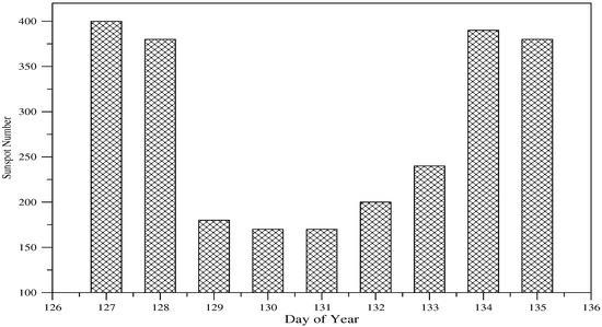
Figure 1.
Temporal variation in daily sunspot numbers from days 127 to 133. The data show distinct peaks around days 127 and 134, corresponding to increased solar activity, while intermediate days exhibit lower sunspot counts.
Figure 2 shows the X-ray flux measurements for the XRS-A (blue) and XRS-B (red) channels from 7 May to 15 May 2024, capturing variations in solar X-ray emissions over this period as recorded by Geostationary Operational Environmental Satellite (GOES-16). These data were accessed from the Space Weather Prediction Center (SWPC) archive on 25 May 2024. Notably, multiple sharp peaks are observed, indicating intense X-ray activity likely associated with solar flares [45,46,47]. The most prominent peak occurs on 14 May 2024, when the XRS-B flux reaches its maximum value of approximately 0.0009 W/m². Across the entire observation period, XRS-B consistently records higher flux values compared to XRS-A, reflecting its sensitivity to higher-energy X-ray emissions.
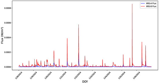
Figure 2.
Solar X-ray flux variations captured by XRS-A and XRS-B channels (7–15 May 2024): highlighting intense X-ray activity with a prominent peak on 14 May, as XRS-B flux reaches 0.0009 W/m².
Figure 3 presents the EUVS irradiance measurements for five distinct wavelength bands—256, 284, 304, 1175, and 1216—from 7 May 2024 to 15 May 2025: irradiance 256 (EUV, Fe XV) has a wavelength of 256 Å, irradiance 284 (EUV, Fe XIV) has a wavelength of 284 Å, irradiance 304 (Helium II, EUV) has a wavelength of 304 Å, irradiance 1175 (Neon emission line, FUV) has a wavelength of 1175 Å, and irradiance 1216 (Lyman-alpha, UV, Hydrogen) has a wavelength of 1216 Å. Each wavelength band exhibits unique trends, with notable differences in magnitude and variability. The 1216 band, represented by the orange curve, demonstrates significantly higher irradiance values compared to the other bands, ranging between approximately 0.008 and 0.010 units. It also shows a gradually increasing trend over the observation period, with minor fluctuations suggesting relatively steady solar activity. In contrast, the 304 band (red curve) maintains a much lower irradiance level while exhibiting slight variations within a narrow range. The remaining bands—256, 284, and 1175—display irradiance values that cluster close to zero, with minimal variation over time.
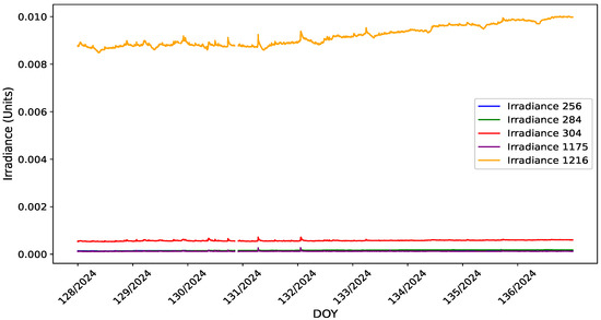
Figure 3.
EUVS irradiance trends across five wavelength bands (7 May 2024–15 May 2025): highlighting the dominant 1216 band (Lyman-alpha, orange curve) with a steady upward trend and irradiance values between 0.008 and 0.010 units, contrasting with the lower and stable outputs of the 304, 256, 284, and 1175 bands.
Figure 4 shows the solar wind characteristics as recorded from NASA’s Advanced Composition Explorer (ACE) Level 2 data archive. We accessed the Solar Wind Proton Density and Speed (SWICS) database on 25 May 2024. The top panel of Figure 4 shows the hydrogen temperature (), revealing fluctuations ranging from K to K, with occasional sharp spikes. The middle panel, depicting the % ratio, serves as a proxy for solar wind composition. The bottom panel shows the solar wind bulk speed () in km/s.
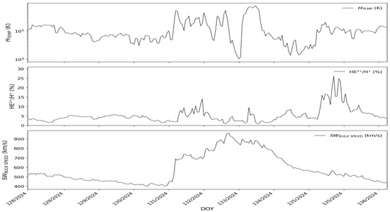
Figure 4.
Solar wind parameters over time, The top panel shows hydrogen temperature () in Kelvin, the middle panel displays the ratio (%), and the bottom panel depicts solar wind bulk speed () in km/s.
During the solar storm, the plasma temperature in the solar wind and Earth’s near-space environment (magnetosphere) can undergo significant variations. Plasma temperature is a key parameter that influences the behavior of the charged particles interacting with Earth’s magnetic field. The solar wind plasma typically has a temperature ranging from 10,000 K to 200,000 K under quiet conditions, depending on solar activity and distance from the Sun. When a CME or an interplanetary shock wave arrives, plasma compression occurs, causing a sharp temperature rise [48,49]. During this mega storm, the first sharp peak of temperature rose up to K on 10 May at around 19:00 UTC (Figure 5). The highest temperature reached K on 12 May at around 17:00 UTC. The intensity of this heating depends on the speed of the solar wind (faster CMEs produce stronger heating) and the density of the plasma. Plasma temperatures gradually returned to normal levels on 13 May at around 00:00 UTC. Proton density during a solar storm depicts the variations in the concentration of protons (charged particles) in the solar wind, measured in particles per cubic centimeter (cm−3). Proton density started increasing on 10 May at 12:00 UTC and reached its maximum value on 10 May at 20:00 UTC. These peaks were observed until 11 May at 12:00 UTC, after which the values returned to normal. The F10.7 index is a measure of solar radio emissions at a wavelength of 10.7 cm (or a frequency of 2800 MHz), and it is a key parameter used in space weather studies. It serves as a proxy for solar activity and is strongly correlated with the sunspot number and the ultraviolet radiation that affects Earth’s ionosphere and thermosphere. The variation in F10.7 from 7 May to 15 May is shown in Figure 5. The Lyman-alpha line (Ly-) is a specific ultraviolet spectral line emitted by hydrogen atoms at a wavelength of 121.6 nm. In space weather studies, it is a significant indicator of solar activity and has a direct impact on Earth’s upper atmosphere [50,51,52]. Lyman-alpha radiation falls within the EUV spectrum and is one of the strongest emission lines from the Sun, especially during periods of high solar activity [53,54]. The value of Lyman-alpha started increasing from 10 May, indicating the beginning of the solar storm and its potential impact on Earth. The variation in Lyman-alpha from 7 May to 15 May is shown in Figure 5.
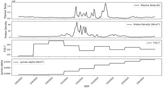
Figure 5.
Variation in plasma temperature (K), proton density (N/cm³), F10.7 index, and Lyman-alpha from 7 May 2024 to 15 May 2024. A noticeable rise and fluctuation in plasma temperature and density are observed between 10 May and 13 May, returning to normal after 13 May. The F10.7 index increases on 8 May and 9 May, followed by a decline after 9 May. Lyman-alpha variation exhibits a stepwise rise from 10 May, continuing its upward trend until 15 May.
The interplanetary magnetic field (IMF), having magnitude B, is a component of the Sun’s magnetic field carried into space by the solar wind. The IMF is critical in shaping space weather and its effects on Earth. The IMF is usually expressed in terms of its components and . The component (in the Geocentric Solar Magnetospheric (GSM) coordinate system) is vital. When is negative (southward), it allows for stronger coupling with Earth’s magnetic field, leading to geomagnetic storms. Variations in IMF B, especially changes in , influence the transfer of energy from the solar wind to Earth’s magnetosphere. Strong IMF B values are associated with intensified space weather events, such as auroras, geomagnetic storms, and disruptions to satellites and communication systems [55,56,57,58,59]. Figure 6 presents the total IMF (first panel) and the three components (second panel), (third panel), and (fourth panel). The values of IMF B began to increase on 10 May at around 18:00, reaching the maximum value of 70 nT before 11 May at 00:00 UTC. Then, they started to decrease and reached a value of 10 nT on 12 May at 06:00. Whereas and reached the value −25 nT and −40 nT, respectively, on 11 May 00:00 UTC, and reached the maximum value 65 nT just before 00.00 UTC on 11 May.
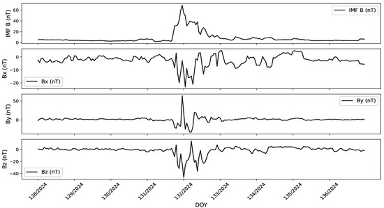
Figure 6.
Interplanetary magnetic field (IMF), the component of the IMF along the Sun–Earth line (), the component perpendicular to the Sun–Earth line, lying in the ecliptic plane (), and the component perpendicular to the ecliptic plane, crucial for geomagnetic activity (), are plotted (in nT) from 7 May to 15 May 2024. A positive peak in IMF and is observed on 11 May, while and show negative peaks.
We have plotted three auroral indices, Auroral Electrojet (AE), Auroral Lower (AL), and Auroral Upper (AU), in Figure 7. These indices are derived from magnetometer data recorded at stations located in the auroral regions. The AE, AL, and AU indices are typically calculated at 1-minute intervals, providing a high-resolution picture of auroral activity. The AE index quantifies the overall strength of auroral electrojet activity. It is derived as the difference between the AU (upper) and AL (lower) indices. A higher AE value indicates stronger auroral activity and greater disturbances in the ionosphere [60]. In this case, the AE index began to increase from 10 May at 00:00 UTC, with several sharp peaks observed between 10 May and 13 May. The AE index reached its maximum value on 11 May at 13:00 UTC. The index returned to normal levels by 15 May at 00:00 UTC. The AL index represents the strength of the westward auroral electrojet, determined from the lowest magnetic field deviation recorded at magnetometer stations in the auroral zone. Westward electrojets occur during substorms and are associated with increased geomagnetic disturbances. A more negative AL value signifies stronger westward currents and higher auroral activity. In this case, the AL index became negative starting from 10 May at 00:00 UTC. After several sharp negative peaks, it reached its lowest value on 11 May around 13:00 UTC. Following additional peaks, the AL index returned to normal levels by 15 May at 00:00 UTC. Lastly, we plotted the Auroral Upper (AU) index, which represents the strength of the eastward auroral electrojet. Eastward electrojets occur during substorms and reflect a distinct part of the ionospheric current system. Higher AU values indicate stronger eastward currents. In this case, the AU index began to rise on 10 May at 00:00 UTC, reaching its highest value on 10 May at 23:00 UTC after several intermediate peaks. Additional sharp peaks were observed between 10 May and 14 May. The AU index returned to normal levels by 15 May at 00:00 UTC.
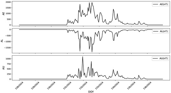
Figure 7.
Temporal variation in auroral indices AE, AL, and AU (in nT) from 7 May to 15 May 2024. AE and AU exhibit multiple enhancements, while AL shows several negative excursions between 10 May and 14 May. The most pronounced peak in all indices is observed on 11 May 2024, indicating intensified auroral activity.
We have plotted Ap, Kp, and, Dst from 7 May to 15 May in Figure 8. The Ap index is a linear measure of daily average geomagnetic activity, derived from the Kp index over 24 h [61]. It typically ranges from a few nanoteslas (nT) to 400 nT or more. On 10 May at 18:00 UTC, the Ap index reached 300 nT, and it peaked at its maximum value on 11 May between 00:00–02:00 UTC and 10:00–11:00 UTC. This indicates an extremely severe geomagnetic storm during that time. The Ap index returned to normal levels by 13 May. The Kp index is a global, quasi-logarithmic measure of geomagnetic activity based on variations in the Earth’s magnetic field recorded by ground-based magnetometers. It ranges from 0 (very quiet) to 9 (extremely disturbed), with higher values indicating stronger geomagnetic activity, often associated with auroras and geomagnetic storms. Here, the Kp index is represented as . On 11 May at 00:00 UTC, the Kp index reached its maximum value of 9 and remained elevated throughout the day. By 12 May at 12:00 UTC, the value dropped to 2, before rising again to 6.3 at 21:00 UTC, after which it declined. The variation in the Kp index indicates an extremely disturbed geomagnetic condition between the 10 and 11 May, followed by moderately disturbed conditions on the 12 May. The Dst index measures the intensity of the ring current in the Earth’s magnetosphere, which develops during geomagnetic storms. On 10 May at 19:00 UTC, a significant drop in the Dst value began, reaching −412 nT by 11 May at 02:00 UTC. A Dst value of −412 nT signifies an extremely severe geomagnetic storm, ranking among the most intense levels of geomagnetic disturbance. While this value reflects a significant storm, it is less severe than the strongest storms in history, such as the Carrington Event of 1859 and the March 1989 geomagnetic storm, both of which caused widespread and notable effects [62,63,64,65]. After the storm day, the Dst value returns to normal slowly after four to five days [66,67].
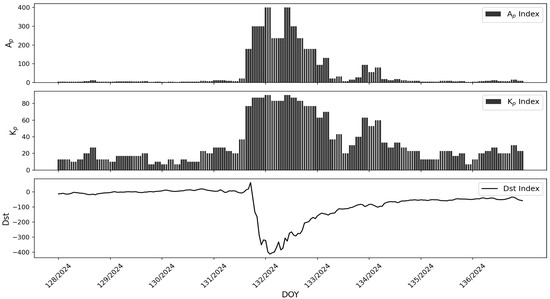
Figure 8.
Temporal variation in planetary indices (Ap, Kp) and Dst values from 7 May to 15 May 2024. Ap and Kp indices, represented as bar graphs, exhibit significant enhancements between 10 May and 13 May, indicating increased geomagnetic activity. The Dst index attains its most negative value on 11 May, suggesting the occurrence of a major geomagnetic storm.
2.3. Data Sources
The IGS stations using the GNSS are a global network of continuously operating reference stations that provide high-precision GNSS data for scientific and geodetic applications. These stations support real-time and post-processed positioning, atmospheric studies, and Earth deformation monitoring. The IGS network contributes to the maintenance of the International Terrestrial Reference Frame (ITRF) and is essential for applications such as precise orbit determination, space weather studies, and geodynamics. The data collected by these stations are publicly available through the IGS data centers, facilitating global research and engineering applications. We have taken 422 stations for analysis, as shown in Figure 9. Due to the unavailability of data, we could not consider all of the GNSS stations. This study utilized the global GNSS-IGS stations (https://cddis.nasa.gov/archive accessed on 1 July 2024) database with a spatial resolution of 2.5° × 5° and a temporal resolution of 15 min. The receiver independent exchange format (RINEX) is a standardized format for raw satellite navigation data, and is designed to allow users to post-process the data for greater accuracy, developed by [68]. RINEX has become a key tool in satellite navigation. It includes three types of ASCII files: observation files containing GPS measurement data, navigation files providing satellite orbit details, and meteorological files with pressure and temperature information.
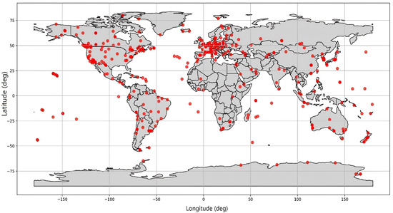
Figure 9.
The location of four hundred and twenty-two GNSS-IGS stations over the globe used for this work.
2.4. Data Analysis
The IGS, established in 1998, focuses on monitoring ionospheric TEC using ground-based GNSS receivers [67]. Its primary aim is to study ionospheric delays and scintillations. To achieve this, the IGS has developed a network of 500 monitoring stations and established four ionospheric associate analysis centers (IACCs): the Centre for Orbit Determination in Europe (CODE), the Jet Propulsion Laboratory (JPL), the European Space Agency (ESA), and the Polytechnic University of Catalonia (UPC). Additionally, the IGS created the Multi-GNSS Experiment (MGEX) network to gather data from multiple satellite systems, including GPS, GLONASS, and BeiDou. This analysis majorly involved the (a) temporal VTEC deviation analysis for selected GNSS stations, (b) global mapping of VTEC anomalies using the GIM database, and (c) comparative study of IGS and GIM datasets for validation.
2.5. Processing of RINEX File Using IGS Data
This study focuses on examining the characteristics of the F-layer of the ionosphere using the TEC as a key parameter during Solar Cycle 24 under normal ionospheric conditions. We will review the methods employed to measure TEC, emphasizing the analysis of data derived from the GPS and GNSS. Additionally, the contribution of the IGS network will be discussed in detail. The ionosphere acts as a dispersive medium for electromagnetic waves. Regular refraction can be estimated under a uniform electron density distribution when a radio signal propagates through it. Suppose the radio signal’s frequency is much higher than the critical frequency of the F-layer and the layer’s thickness is negligible compared to its radius of curvature. In that case, the refraction primarily depends on the signal frequency and the TEC. For modeling the ionosphere, the electron density profile is a fundamental parameter. It offers a direct means of investigating the ionosphere’s structure, variability, and effects on radio wave propagation. TEC is an essential factor for understanding ionospheric phenomena because it plays a significant role in describing the interaction of the ionosphere with radio waves. It is widely utilized to determine the ionosphere’s status and structure. TEC represents the total number of free electrons along a vertical column from the ground to approximately 1000 km above Earth. Often referred to as “columnar electron density”, TEC is expressed in TEC units (TECUs), where 1 TECU is equivalent to electrons per square meter. The slant total electron content (STEC) measures the total number of free electrons in a column of the unit cross-section along the electromagnetic wave path between the satellite and the receiver. As STEC depends on the ray path geometry through the ionosphere, it is desirable to calculate an equivalent vertical value of TEC, which is independent of the elevation of the ray path. The VTEC is obtained by taking the projection from the slant to the vertical using a mapping function technique or an obliquity factor (M(χ)) at a certain height known as the ionospheric pierce point (IPP) [22,69,70]. This can be expressed as the following:
We downloaded daily CRX and RNX files from the CDDIS website (https://urs.earthdata.nasa.gov accessed on 15 July 2024) for days 128 to 136 of the year 2024, with days 131 and 132 identified as storm days. These files were organized by station and subsequently converted into STD files using the software Gopi Seemala GPS-TEC Program Ver 2.9.5 developed by Dr. Gopi Krishna Seemala (https://seemala.blogspot.com accessed on 5 August 2024). This software requires observation, navigation, and code bias files as inputs. The program code and its application for VTEC computation have been discussed in several key studies. In our approach, we aimed to convert the STEC into an equivalent VTEC by applying thin-shell approximation and the technique outlined in [71,72,73]. Following this, we selected 20 conjugate grid points across the global map, ensuring that each pair shares the same longitude and nearly identical latitudes in both hemispheres. We then generated time versus VTEC plots for each grid point station for days 129, 131, 132, and 136. Next, we studied the longitude-wise variation in VTEC. To do this, we first divided the stations into latitude bands of 0–10°, 10–20°, 20–30°, 30–40°, 40–50°, 50–60°, 60–70°, and 70–80° in both the Northern and Southern Hemispheres. Then, we calculated the average VTEC at 0, 6, 12, and 18 UTC for each station. We plotted the average VTEC of the stations against longitude for each case and also compared these longitude-wise VTEC variations with GIM data.
3. Results
3.1. Temporal Variations in Ionospheric Distribution at Low Latitudes
Figure 10 presents time-series plots from multiple GNSS-IGS observation stations worldwide, capturing variations in VTEC measured in TECU over time (in UTC) during the storm period. The plots show the diurnal variation in VTEC for 20 GNSS-IGS stations (see Table 1) for DoY 129 (black), 131 (red), 132 (green), and 136 (blue). The x-axis represents the time in UTC, while the y-axis represents VTEC values. Each sub-figure corresponds to a different station, showing the response of the ionosphere to the geomagnetic storm at that location. Each plot contains four different curves, corresponding to specific time periods during the storm. The black curve (Day 129) represents pre-storm conditions, serving as a baseline for our comparison. It captures typical ionospheric behavior under quiet space weather conditions. The red curve (Day 131) depicts the VTEC at the storm’s initial phase when geomagnetic disturbances begin affecting the ionosphere. This captures the early ionospheric response to penetration electric fields and changes in neutral dynamics. The green curve (Day 132) represents the peak of the storm, showing maximum ionospheric disturbance where the VTEC variations during this phase result from strong electric fields, ionospheric currents, and thermospheric changes. The blue curve (Day 136) shows the post-storm ionospheric recovery, when VTEC returns to quiet-time conditions. At this stage, the ionosphere stabilizes as storm-driven electric fields and neutral winds subside. The overall sub-figures give a comprehensive view of the spatio-temporal variations of VTEC profiles that depend on the storm times, station’s location, local time, and the background solar-driven characteristics. The key observations from Figure 10 can be explained as the following:
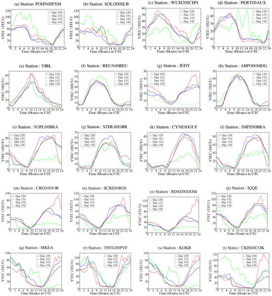
Figure 10.
VTEC (TECU) time series variation (hours) for twenty grid points across different regions of Earth. The black line represents the pre-storm day (DoY 129), while the red and green lines represent the storm days (DoY 131 and 132). The blue line indicates the post-storm day (DoY 136).

Table 1.
List of selected grid points (IGS stations) and their longitude and latitude.
- Strom-driven VTEC enhancements and depletions: Both the positive (increment) and negative (depletion) storm effects are observed in the VTEC variations [74,75,76,77]. For the positive storm effects, stations such as POHN0FSM, SOLO0SLB, WUH20CHN, and REUN0REU show a significant increase in VTEC during the storm (green curve (Day 132) is much higher than black (Day 129)). This is due to penetration electric fields (PEFs), which lift ionospheric plasma to higher altitudes where recombination rates are lower, leading to an increase in VTEC [78,79,80,81,82,83]. Some stations, including CYNED0GUF, CRO10VIR, and SCRZ0BOL, exhibit a decrease in VTEC (green curve lower than black). VTEC values across different stations varied markedly, with daytime peaks dropping from 60–90 TECU to as low as 10–20 TECU at depletion phases (a 60–80% decrease), while enhancements at certain locations reached 100–120 TECU (a 30–50% increase). These variations, corresponding to electron density changes of approximately – cm−3 in the F2 layer, reflect the combined effects of penetration electric fields, disturbance dynamo processes, and storm-induced thermospheric composition changes on ionospheric plasma redistribution. This is likely due to storm-driven equatorward neutral winds, which bring in molecular-rich air (N2, O2), enhancing recombination and reducing electron density [84,85,86,87,88].
- Variation based on local time dependency: The plots reveal a strong diurnal pattern, with VTEC peaking around local noon due to solar-driven ionization. Some stations (e.g., KOKB, THFG0PYF) show post-sunset VTEC enhancements, which are likely due to storm-driven plasma transport, penetration electric fields (PEFs), or storm-enhanced density (SED) [89,90,91,92]. These effects cause plasma redistribution, particularly at mid-latitudes and high-latitudes, leading to increased electron density in certain regions [93,94].
- Regional variability: The low-latitude stations (e.g., POHN0FSM, SOLO0SLB) show stronger positive storm effects due to the equatorial fountain effect [95,96,97,98,99,100,101,102,103,104], where plasma is lifted and redistributed, whereas high-latitude stations (e.g., CKIS0COK) exhibit more irregular fluctuations, likely caused by auroral precipitation [105,106] and ionospheric convection effects [107,108,109,110,111]. The overall variation can be explained through multiple solar-terrestrial phenomena that lead to upper ionospheric irregularities. At the storm’s onset (red curve, Day 131), strong interplanetary electric fields penetrate into the ionosphere, causing plasma redistribution; this results in increased VTEC at low latitudes due to upward plasma transport. In the post-storm period (blue curve, Day 136), ionospheric winds and currents are altered, leading to reduced VTEC at some locations due to disturbance dynamo effects (DDEs) in the recovery phase. Most importantly, the storm changes the thermoionic ratio, enhancing recombination in some regions and leading to localized VTEC depletion. Some stations clearly show wave-like oscillations in VTEC, which may indicate the generation of TIDs caused by storm-induced gravity waves [112,113].
3.2. Global VTEC Anomalies
Figure 11 illustrates the longitudinal variations in VTEC at two Universal Time (UT) epochs (00:00 UT and 12:00 UT) across four different days of the year (DoY): 129, 131, 132, and 136, capturing the ionospheric response before, during, and after the G5 geomagnetic storm of 11–12 May 2024. The VTEC variations are plotted for two sets of latitude ranges. The blue curves represent the Northern Hemisphere latitudes (0 to 10°, 0 to 20°, 0 to 30°, and 0 to 40°) (left to right), and the red curves represent the Southern Hemisphere latitudes (0 to −10°, 0 to −20°, 0 to −30°, and 0 to −40°) (left to right). This dataset provides insights into the storm-time ionospheric response in terms of latitude, longitude, and UT variations.
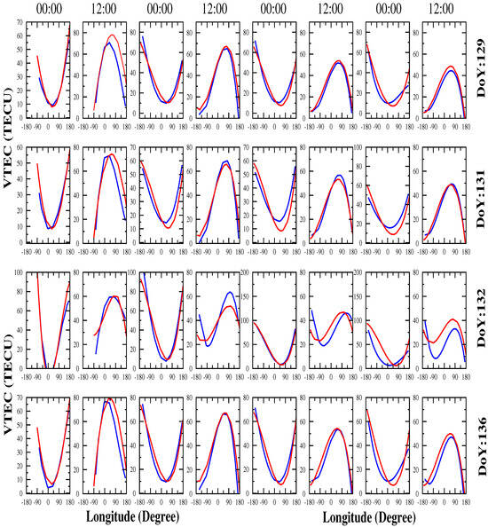
Figure 11.
Longitudinal variations of VTEC across different latitude ranges: 0–10° (1st and 2nd columns), 0–20° (3rd and 4th columns), 0 –30° (5th and 6th columns), and 0–40° (7th and 8th columns) at UTC 00:00 and 12:00. The blue and red lines represent VTEC variations in the Northern and Southern Hemispheres, respectively, measured in TECU. Rows correspond to different storm phases: pre-storm day (1st row), storm days (2nd and 3rd rows), and post-storm day (4th row).
- Pre-storm conditions (DoY 129): The VTEC distribution follows a diurnal pattern, where values increase during the daytime (12:00 UT) and decrease during nighttime (00:00 UT). The blue and red curves are relatively symmetric, indicating a balanced electron density distribution between hemispheres under quiet geomagnetic conditions. The VTEC peaks occur around equatorial and low-latitude regions, consistent with the equatorial ionization anomaly (EIA) [104,114,115], driven by the fountain effect [116]. The longitudinal variations are smooth and consistent, showing no major perturbations.
- Main storm phase (DoY 131–132):
- 1.
- Storm-induced longitudinal asymmetry: A significant longitudinal perturbation emerges during the storm, disrupting the usual smooth variation in VTEC. At 00:00 UT, the blue curves (Northern Hemisphere) show a sharp depletion in VTEC at specific longitudes, while the red curves (Southern Hemisphere) exhibit relative enhancement. At 12:00 UT, VTEC enhancements in the Northern Hemisphere become more pronounced, especially near 45° to 90° and ±180° longitude, suggesting storm-enhanced density (SED) formation. The longitudinal variability is more intense at mid-latitudes, where storm-driven electric fields and thermospheric winds play a dominant role in redistributing ionospheric plasma [117,118,119]. From Figure 12, at 06:00 UT, a noticeable depletion is observed in the Southern Hemisphere (red curves) compared to the Northern Hemisphere (blue curves). At 18:00 UT, the Northern Hemisphere shows an increase in VTEC, particularly at longitudes 45° to 90° and ±180°, indicative of storm-enhanced density (SED) regions. The sharp latitudinal and longitudinal gradients suggest the presence of penetration electric fields and TIDs [120,121,122].
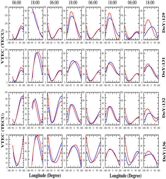 Figure 12. Longitudinal variations of VTEC across different latitude ranges: 0–10° (1st and 2nd columns), 0–20° (3rd and 4th columns), 0–30° (5th and 6th columns), and 0–40° (7th and 8th columns) at UTC 06:00 and 18:00. The blue and red lines represent VTEC variations in the Northern and Southern Hemispheres, respectively, measured in TECU. Rows correspond to different storm phases: pre-storm day (1st row), storm days (2nd and 3rd rows), and post-storm day (4th row).
 - 2.
- Hemispheric differences in VTEC response: The blue (Northern Hemisphere) curves show a positive storm effect (VTEC enhancement), whereas the red (Southern Hemisphere) curves show a negative storm effect (VTEC depletion). This asymmetry is likely due to the combined impact of penetration electric fields, disturbance dynamo effects, and thermospheric composition changes [123]. At higher latitudes (30–40° in both hemispheres), the deviations are more pronounced, indicating a strong influence of storm-time ionospheric currents [124] and neutral wind effects [125]. At 06:00 UT and 18:00 UT, the Northern Hemisphere (blue) experiences a positive storm effect (VTEC enhancement) whereas the Southern Hemisphere (red) experiences a negative storm effect (VTEC depletion). This asymmetry possibly arises due to the penetration of electric fields, which redistribute ionospheric plasma, have disturbance dynamo effects, and alter plasma transport and thermospheric composition changes, affecting ionization–recombination balance [126,127].
- Post-storm recovery (DoY 136): The VTEC distribution begins to return to pre-storm levels, but some residual disturbances persist, particularly in the mid-longitude sectors (±90° and ±180°). The recovery process is latitude-dependent, with the equatorial and low-latitude regions recovering faster, while higher latitudes show delayed restoration. The asymmetry between the red and blue curves decreases, indicating a gradual re-establishment of hemispheric balance in electron density. At 06:00 UT and 18:00 UT, the VTEC starts returning to pre-storm levels, but residual perturbations persist, particularly around 45° to 90° and ±180° longitude. The hemispheric symmetry begins to re-establish, indicating gradual ionospheric stabilization. The VTEC for higher latitudes recovers more slowly, while low latitudes exhibit a faster return to normal conditions due to the equatorial fountain effect. The higher latitudes (30–40°) exhibit stronger deviations, showing the impact of storm-induced electric fields and neutral wind dynamics, whereas the lower latitudes (0–10°) maintain a relatively stable structure, dominated by equatorial plasma transport processes.
The storm introduces latitudinal and longitudinal differences in VTEC, reflecting the interplay between electric fields, neutral winds, and geomagnetic field interactions. The Northern Hemisphere experiences stronger positive storm effects, likely due to the dominant penetration electric field direction. The Southern Hemisphere shows stronger negative storm effects, possibly due to increased molecular nitrogen (N2) and oxygen (O) upwelling, leading to enhanced recombination and electron density depletion [128,129]. The storm effects are stronger at certain longitudes, especially near 45° to 90° and ±180°, suggesting that geomagnetic activity has region-specific influences on ionospheric plasma redistribution [130]. This analysis demonstrates the significant impact of the 11–12 May 2024 G5 geomagnetic storm on longitudinal and latitudinal variations in VTEC. The study confirms strong longitudinal variations, particularly at 45° to 90° and ±180° longitudes. A significant hemispheric asymmetry is observed, with positive storm effects in the Northern Hemisphere and negative effects in the Southern Hemisphere. The higher latitudes exhibit prolonged recovery, while equatorial regions return to normal faster. The storm-induced electric fields, thermospheric changes, and neutral wind effects significantly influence the VTEC dynamics, producing a wide range of variations.
This comparative study analyzes VTEC variation at four key Universal Time Coordinated (UTC) epochs: 00:00, 06:00, 12:00, and 18:00 UTC, using the two figures provided. The analysis focuses on the changes in longitudinal and hemispheric VTEC distributions before, during, and after the G5 geomagnetic storm of 11–12 May 2024.
3.3. Overview of VTEC Variation Across Time
At 00:00 UTC and 06:00 UTC (nighttime/morning hours), lower VTEC values are observed due to reduced ionization caused by the absence of solar radiation. The storm effects are prominent in the Southern Hemisphere, leading to asymmetric behavior. On the contrary, at 12:00 UTC and 18:00 UTC (daytime/afternoon hours), higher VTEC values are observed due to peak ionization from solar radiation. The storm-induced perturbations are most noticeable in the post-noon sector (18:00 UTC), with a hemispheric asymmetry present, particularly at mid-latitudes.
In the pre-storm conditions, the VTEC follows a diurnal cycle: lower at night and higher during the daytime. During the onset and storm period, the Southern Hemisphere (red) experiences significant depletion at night, while the Northern Hemisphere (blue) exhibits enhanced VTEC during the day. In the post-storm situation, the nighttime VTEC remains slightly suppressed, while daytime values start to return to normal. A prominent storm-time hemispheric difference is observed from the figures. In the Northern Hemisphere, positive storm effects (VTEC increase) are observed; whereas, in the Southern Hemisphere, the effects are negative in nature (VTEC decrease). The maximum disturbance occurs at 18:00 UTC, with the strongest VTEC deviations at 45° to 90° and ±180° longitude. The longitudinal variations are quite interesting. The VTEC shows a smoother distribution before the storm. During the storm, sharp gradients develop, particularly at 45° to 90° and ±180° longitude. During the post-storm period, these longitudinal variations begin to dissipate, but full recovery is not immediate.
The storm significantly altered the natural VTEC diurnal pattern, with asymmetry between hemispheres. The maximum storm-induced disturbances occurred at 18:00 UTC, whereas the strongest depletions were observed at 06:00 UTC. The post-storm recovery is gradual, with residual effects still visible at 00:00 UTC and 06:00 UTC on DoY 136 [131,132,133]. The comparative overview is given in the Table 2.
Table 2.
Comparison of VTEC variations at different UTC epochs before, during, and after the storm.
3.4. Outcomes of GIM Observation
Figure 13 and Figure 14 present the longitudinal variations of VTEC at four UT epochs (00:00 UT, 06:00 UT, 12:00 UT, and 18:00 UT) across four different days of the year (DoY): 129 (pre-storm), 131 (storm onset), 132 (main storm phase), and 136 (recovery phase). The red curves indicate VTEC variations for the Northern Hemisphere latitudes (0° to 40°), while the blue curves represent the Southern Hemisphere latitudes (0° to −40°). This dataset, derived from GIM, provides insights into the ionospheric response during and after the G5 geomagnetic storm of 11–12 May 2024 [134,135].
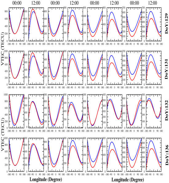
Figure 13.
Longitudinal variations of VTEC across different latitude ranges: 0–10° (1st and 2nd columns), 0–20° (3rd and 4th columns), 0–30° (5th and 6th columns), and 0–40° (7th and 8th columns) at UTC 00:00 and 12:00, from the GIM database. The blue and red lines represent VTEC variations in the Northern and Southern Hemispheres, respectively, measured in TECU. Rows correspond to different storm phases: pre-storm day (1st row), storm days (2nd and 3rd rows), and post-storm day (4th row).
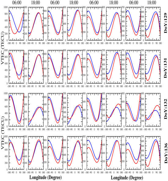
Figure 14.
Longitudinal variations of VTEC across different latitude ranges: 0–10° (1st and 2nd columns), 0–20° (3rd and 4th columns), 0–30° (5th and 6th columns), and 0–40° (7th and 8th columns) at UTC 06:00 and 18:00, from the GIM database. The blue and red lines represent VTEC variations in the Northern and Southern Hemispheres, respectively, measured in TECU. Rows correspond to different storm phases: pre-storm day (1st row), storm days (2nd and 3rd rows), and post-storm day (4th row).
3.4.1. Temporal Evolution of VTEC (Before, During, and After the Storm)
- Pre-storm condition (DoY 129): The VTEC follows a typical diurnal cycle with higher values at 12:00 UT and lower values at 00:00 UT. The VTEC variations at 06:00 UT show lower ionization levels as the ionosphere is still in the early morning phase. At 18:00 UT, the VTEC increases significantly due to peak daytime ionization from solar EUV radiation. The latitudinal variations show a nearly symmetrical distribution between the Northern and Southern Hemispheres. The longitudinal variations indicate smooth and predictable trends, with peak VTEC values centered near the equatorial regions. In the morning phase, the VTEC starts to increase in the Northern Hemisphere, especially around equatorial regions [104,114,115].
- Storm onset (DoY 131): The onset condition of the storm introduces a significant asymmetry between the hemispheres. A noticeable increase in VTEC is observed in the Northern Hemisphere, particularly around the equatorial anomaly regions. The Southern Hemisphere exhibits a reduction in VTEC due to ionospheric depletion, which may be linked to enhanced electrodynamic forcing and redistribution of plasma via storm-induced electric fields. In the evening, the ionospheric enhancement becomes more pronounced, particularly in the Northern Hemisphere, which suggests the onset of a positive storm effect (VTEC enhancement due to electric field penetration and disturbed dynamo effects). The Southern Hemisphere exhibits early signs of depletion, marking the beginning of a negative storm effect caused by increased recombination [117,118,119].
- Main storm phase (DoY 132): In the morning, the strongest perturbations occur, with a significant VTEC enhancement in the Northern Hemisphere and continued depletion in the Southern Hemisphere. In the evening, the positive storm effect becomes more evident in the Northern Hemisphere, reaching higher VTEC levels compared to the pre-storm period. Sharp longitudinal gradients develop, particularly at ±90° and ±180° longitude, indicating enhanced EIA driven by storm-time electric fields. The latitudinal asymmetry is further amplified, possibly due to differences in storm-time thermospheric winds and inter-hemispheric plasma transport [120,121,122].
- Post-storm recovery (DoY 136): The VTEC distribution begins to return to normal but retains residual storm effects. In the morning, VTEC starts to return to normal levels but still exhibits asymmetries due to lingering storm effects, while in the evening, the recovery is more evident in both hemispheres, though some perturbations persist, especially at certain longitudes where storm-induced anomalies take longer to dissipate. A slower recovery is observed in the Southern Hemisphere, while the Northern Hemisphere still exhibits slightly elevated VTEC levels. The longitudinal variations remain somewhat disturbed, indicating that complete recovery from the geomagnetic storm is still in progress.
3.4.2. Latitudinal Dependence of VTEC Variations
The latitudinal dependence of VTEC during the geomagnetic storm of 11–12 May 2024, reveals significant asymmetries between the Northern and Southern Hemispheres, with variations strongly tied to the time of day, geomagnetic activity, and storm-driven ionospheric dynamics. At night (00:00 UT), before the storm, VTEC follows a smooth diurnal pattern, with low electron densities due to the absence of solar radiation. However, during the storm (DoY 131–132), a strong negative storm effect appears in the Southern Hemisphere, where enhanced molecular oxygen and nitrogen increase recombination, leading to VTEC depletion. In contrast, the Northern Hemisphere experiences slight enhancements, possibly due to storm-driven penetration electric fields that push plasma to higher altitudes, slowing recombination. As the storm subsides (DoY 136), the Southern Hemisphere remains more depleted than the Northern Hemisphere, indicating an asymmetric recovery process.
In the morning (06:00 UT), storm effects become more pronounced. The Southern Hemisphere experiences its most severe depletion, as the combined effects of storm-induced compositional changes and natural morning decay further reduce VTEC. Meanwhile, in the Northern Hemisphere, VTEC enhancements start to appear, driven by electric field penetration and thermospheric winds redistributing plasma. At noon (12:00 UT), when solar activity is at its peak, the Northern Hemisphere shows a strong positive storm effect, with elevated VTEC levels due to plasma uplift and delayed recombination. The Southern Hemisphere, on the other hand, continues to show depletion. By the evening (18:00 UT), the Northern Hemisphere enhancements persist, while the Southern Hemisphere begins a slow recovery but still remains below pre-storm levels. The overall storm-time VTEC variations highlight the complex interactions between solar radiation, geomagnetic disturbances, and ionospheric dynamics, leading to highly latitude-dependent and time-sensitive ionospheric responses [128,129].
3.4.3. Longitudinal Variations and Storm-Time Impact
The longitudinal variations of VTEC during the geomagnetic storm of 11–12 May 2024 display distinct storm-induced disruptions across different times of the day, reflecting the interplay between electric fields, thermospheric winds, and geomagnetic activity. Before the storm (DoY 129), at all time epochs—night (00:00 UT), morning (06:00 UT), noon (12:00 UT), and evening (18:00 UT)—the longitudinal distribution of VTEC follows a smooth wave-like structure, with peaks around the equatorial ionization anomaly regions. These variations are primarily driven by solar-controlled ionospheric tides and the equatorial fountain effect. However, as the storm commences (DoY 131–132), the longitudinal VTEC patterns become significantly disrupted, particularly around ±90° and ±180° longitudes, where sharp gradients emerge. These disruptions suggest the presence of penetration electric fields and disturbance dynamo effects, which alter equatorial plasma transport and redistribute ionization. The Northern Hemisphere exhibits strong positive storm effects, with enhanced VTEC values due to plasma uplift and prolonged electron lifetimes at higher altitudes. In contrast, the Southern Hemisphere undergoes significant depletion, reflecting storm-induced compositional changes that enhance recombination and reduce electron density.
At night (00:00 UT), the storm-driven electric fields create noticeable plasma redistribution, leading to asymmetrical longitudinal structures. In the morning (06:00 UT), the Southern Hemisphere shows the most pronounced depletion, while the Northern Hemisphere starts exhibiting plasma uplift-induced enhancements. By noon (12:00 UT), when solar radiation is strongest, the Northern Hemisphere experiences peak storm-induced enhancements, particularly at critical longitudes (±90° and ±180°), where storm effects amplify equatorial ionization anomalies. In the evening (18:00 UT), as the storm weakens, longitudinal gradients begin to smooth out, but lingering storm-time effects persist, particularly in the Southern Hemisphere, which continues to recover more slowly. By DoY 136 (recovery phase), the longitudinal structure begins returning to pre-storm conditions, yet residual perturbations remain, highlighting the extended impact of thermospheric disturbances. The overall storm response underscores the crucial role of longitudinal asymmetries, electric field penetration, and hemispheric differences in shaping ionospheric storm-time behavior.
The observed storm-time variations in VTEC can be attributed to several key ionospheric mechanisms. Penetration electric fields play a crucial role during geomagnetic storms, as intense interplanetary electric fields penetrate the Earth’s ionosphere, altering plasma transport and enhancing equatorial plasma densities in the Northern Hemisphere while depleting VTEC in the Southern Hemisphere. Additionally, neutral wind effects contribute to plasma redistribution by transporting ionospheric plasma across magnetic field lines, leading to asymmetries between hemispheres. Composition changes further influence VTEC variations, as storm-induced increases in molecular species such as O2 and N2 enhance recombination in the Southern Hemisphere, causing depletion, whereas storm-driven plasma uplift in the Northern Hemisphere reduces recombination rates, leading to sustained VTEC enhancements. Lastly, magnetospheric–ionospheric coupling modifies magnetospheric currents, which in turn influence ionospheric electrodynamics, shaping the overall variations observed during the storm.
The figures provides key insights into the ionospheric response to the intense G5 geomagnetic storm of 11–12 May 2024, revealing strong hemispheric asymmetries. The Northern Hemisphere experiences a positive storm effect with VTEC enhancements, while the Southern Hemisphere undergoes depletion due to negative storm effects. The most significant perturbations occur at the storm’s peak (DoY 132), with amplified longitudinal variations around ±90° and ±180° longitudes. Recovery begins by DoY 136, though lingering effects persist, particularly in the Southern Hemisphere. These variations are primarily driven by storm-time electric field penetration, neutral wind effects, and composition changes, emphasizing the profound impact of geomagnetic storms on ionospheric dynamics [131,132,133].
Figure 15 illustrates the variations in penetration electric fields (PEFs) (green) and quiet-time electric fields (purple) during the storm (https://geomag.colorado.edu). A strong spike in PEFs on 11 May, coinciding with the storm’s main phase, reflects intense magnetospheric–ionospheric coupling. These fluctuations indicate prompt penetration electric fields (PPEFs), which rapidly uplift plasma to higher altitudes, reducing recombination and causing VTEC enhancements at low latitudes. In contrast, disturbance dynamo electric fields (DDEFs) develop over time, modifying global plasma distribution and leading to prolonged VTEC depletions [79,136,137].
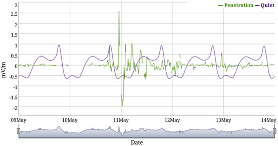
Figure 15.
Variation of penetration electric fields (PEFs) (green) and quiet-time electric fields (purple) from 9 May 2024 to 14 May 2025, illustrating fluctuations associated with geomagnetic activity and ionospheric responses.
Figure 16 presents global maps of the thermospheric O/N2 ratio derived from GUVI (https://guvitimed.jhuapl.edu/guvi-galleryl3on2 accessed on 14 November 2024) observations for 9, 10, 11, and 13 May 2024, capturing the ionospheric–thermospheric response to the intense G5 geomagnetic storm around Mother’s Day 2024. The O/N2 ratio serves as a crucial indicator of energy deposition and neutral composition changes in the upper atmosphere, which directly influences the VTEC variations observed in ionospheric studies. In the pre-storm conditions (9 May 2024), the O/N2 ratio distribution exhibits a relatively stable and typical pattern, with higher values (0.6–1.0) in the low-latitude regions and lower values (0.2–0.4) at higher latitudes. In the main storm phase (10–11 May 2024), a significant depletion in O/N2 is evident in the mid-to-high latitudes, particularly in the Southern Hemisphere, indicating enhanced auroral energy input and thermospheric upwelling, which leads to increased molecular nitrogen and reduced atomic oxygen densities. During the main storm phase, the ratio drops significantly, especially in the Southern Hemisphere and some equatorial regions, with values reducing to approximately 0.4 to 0.8. This represents a 30% to 60% decrease compared to pre-storm values, which is consistent with the expected storm-time upwelling of molecular-rich air ( and ) from the lower thermosphere. In the recovery phase, the ratio begins to return to 1.0 to 1.2, indicating a gradual restoration of thermospheric composition. In summary, the variation in the ratio is at the order of magnitude of from approximately 1.2 to 1.4 (pre-storm) to approximately 0.4 to 0.8 (storm peak): a 30% to 60% decrease.
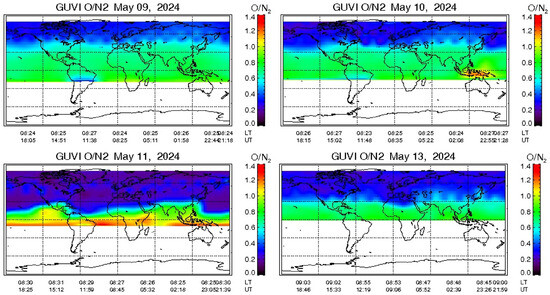
Figure 16.
Global maps of the thermospheric O/N2 ratio for 9, 10, 11, and 13 May 2024, depicting the ionospheric–thermospheric response to the intense G5 geomagnetic storm around Mother’s Day 2024.
The observed depletion in mid-to-high latitudes aligns with expected reductions in VTEC due to increased molecular nitrogen presence and enhanced recombination rates. Conversely, equatorial regions experience transient VTEC enhancements due to storm-driven electrodynamics. This analysis underscores the critical role of thermospheric composition changes in modulating the ionospheric response to extreme geomagnetic storms and highlights the coupling between neutral and ionized atmospheric components during space weather disturbances [112,113,138,139].
3.5. Spatiotemporal Evolution of Peak VTEC Globally
Figure 17 illustrates the spatio-temporal evolution of peak VTEC globally, derived from IGS station data, across four distinct days of the year (DoY 129, 131, 132, and 136). This dataset captures the ionospheric response to the Mother’s Day G5 geomagnetic storm (May 2024), emphasizing significant plasma perturbations driven by extreme space weather conditions [140,141,142].
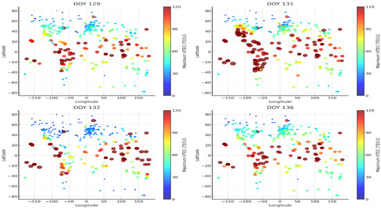
Figure 17.
Spatiotemporal evolution of peak VTEC globally on DoY 129, 131, 132, and 136, derived from IGS station data. The dataset captures ionospheric perturbations during the Mother’s Day G5 geomagnetic storm (May 2024). PPEFs drive intense VTEC enhancements during the main phase, while DDEFs and thermospheric composition changes lead to post-storm depletion. Recovery phase patterns highlight lingering ionospheric disturbances and delayed neutral wind effects.
On DoY 129, the pre-storm state shows relatively moderate VTEC levels, with a balanced distribution of low-to-high electron content values. However, as the storm strengthens, DoY 131 (the storm’s main phase) reveals a dramatic increase in VTEC, particularly in low-latitude and equatorial regions (indicated by numerous deep red clusters). This surge is primarily caused by PPEFs, which drive enhanced equatorial plasma uplift and intensify the EIA. The storm-time electric fields significantly alter the ionospheric structure, redistributing plasma and leading to localized enhancements in ionization.
Following the peak storm phase, DoY 132 shows a sharp decline in VTEC, especially in high-latitude and mid-latitude regions, where blue and cyan markers are prevalent. This depletion is likely due to the combined effects of DDEFs and changes in thermospheric composition, particularly the storm-induced depletion, as corroborated by GUVI observations. The increase in molecular nitrogen at high altitudes enhances plasma recombination, further contributing to the ionospheric depression [143].
By DoY 136, during the recovery phase, we observe a mixed response: some regions display lingering VTEC depletion, while others show pockets of persistent enhancements. These residual effects may be linked to thermospheric recovery processes, post-storm neutral wind circulation, and the delayed impact of disturbance dynamo effects that continue to influence ionospheric densities over several days. Overall, this dataset underscores the storm’s profound impact on ionospheric dynamics, illustrating how extreme geomagnetic activity can induce complex global-scale plasma redistribution.
4. Discussion
This study provides a comprehensive analysis of the ionospheric response to an extreme geomagnetic storm, revealing key spatial and temporal characteristics of VTEC disturbances. The pronounced hemispheric asymmetry, longitudinal variations, and prolonged recovery phase highlight the complexity of storm-time ionospheric dynamics. These findings contribute to the broader understanding of space weather impacts on the ionosphere and emphasize the need for continued advancements in predictive modeling to safeguard GNSS-dependent technologies. The findings of this study highlight the significant ionospheric perturbations induced by the G5 geomagnetic storm of 10–11 May 2024, with a particular emphasis on spatial and temporal variations in VTEC. The observed hemispheric asymmetries and longitudinal variations provide critical insights into the mechanisms governing storm-time ionospheric dynamics.
- Key geomagnetic indices and their storm-time variations: The geomagnetic storm’s intensity and impact were characterized using various indices, as illustrated in Figure 1, Figure 2, Figure 3, Figure 4, Figure 5, Figure 6, Figure 7 and Figure 8. The Dst index reached a minimum of −412 nT, indicating an extremely severe geomagnetic event. This sharp drop in Dst reflects the intensification of the ring current due to enhanced energetic particle injection. Concurrently, the planetary Kp index peaked at 9, highlighting the widespread geomagnetic disturbance affecting the entire ionosphere. The auroral electrojet indices (AE, AL, AU) demonstrated substantial variations, with AE reaching peak values, signifying intense auroral currents driven by enhanced magnetospheric convection. The negative excursion of AL and the concurrent increase in AU confirm significant storm-time substorm activity, which contributed to irregular ionospheric plasma redistribution. Solar activity parameters such as sunspot numbers and X-ray flux (Figure 1 and Figure 2) exhibited noticeable fluctuations preceding the storm. The increased X-ray flux from active regions led to enhanced photoionization, contributing to pre-storm ionospheric variations. The solar wind parameters (Figure 3 and Figure 4) showed sharp increases in solar wind speed and density, with IMF Bz turning strongly southward, triggering reconnection and facilitating storm onset. Additionally, variations in the Lyman-alpha and F10.7 indices (Figure 5) suggest enhanced EUV radiation, further influencing the ionospheric response. The interplanetary magnetic field (IMF) components (Figure 6) showed strong fluctuations, with negative Bz values enhancing magnetospheric coupling. Finally, the planetary Ap index and Kp index (Figure 7 and Figure 8) provided further confirmation of extreme geomagnetic activity, correlating well with the observed ionospheric disturbances.
- Hemispheric asymmetry and geophysical drivers: One of the most striking observations in this study is the pronounced hemispheric asymmetry in ionospheric response. The Northern Hemisphere exhibited positive storm effects characterized by enhanced VTEC, whereas the Southern Hemisphere experienced significant depletion. This asymmetry is primarily attributed to the influence of PPEFs and DDEFs, which modulate plasma redistribution in the ionosphere. The dominance of PPEFs during the main phase of the storm led to increased plasma uplift in equatorial and mid-latitude regions, whereas DDEFs, active during the recovery phase, contributed to the prolonged depletion of VTEC in the Southern Hemisphere due to enhanced recombination processes facilitated by molecular nitrogen upwelling.
- Longitudinal variability and EIA disruptions: The study also revealed significant longitudinal variations, particularly at ±90° and ±180° longitudes, where the storm exerted the strongest impact. These regions exhibited highly amplified longitudinal gradients, disrupting the classical structure of the EIA. The severe modifications in the EIA can be linked to enhanced storm-time electric fields and thermospheric composition changes, which led to an uneven distribution of ionospheric plasma across different longitudinal sectors. These disruptions have profound implications for satellite-based navigation and communication systems as they introduce additional uncertainties in ionospheric delay corrections.
- Temporal evolution and recovery dynamics: The temporal evolution of the storm’s effects demonstrates a complex interplay between different geophysical mechanisms. The storm’s peak impact on day of the year (DoY) 132 was marked by the most intense VTEC disturbances, followed by a gradual recovery phase extending up to DoY 136. While low-latitude regions showed relatively rapid stabilization due to equatorial plasma fountain effects, high-latitude areas exhibited a prolonged recovery period, indicating the lingering influence of thermospheric wind-driven plasma transport. The persistence of post-storm VTEC anomalies suggests that storm-induced perturbations extend well beyond the main event and necessitate continued monitoring for several days.
The results of this study underscore the necessity of improving space weather forecasting models to account for storm-induced ionospheric anomalies. The observed VTEC fluctuations, particularly in low- and mid-latitude regions, pose a substantial challenge for GNSS-based applications, including precise positioning and communication. Enhanced modeling of PPEFs, DDEFs, and thermospheric composition changes will be crucial for mitigating the adverse effects of geomagnetic storms on technological infrastructure.
5. Conclusions
The G5 geomagnetic storm of 10–11 May 2024 provided a unique opportunity to analyze large-scale ionospheric disturbances using high-resolution GNSS-IGS and GIM datasets. This study reveals significant storm-induced perturbations in VTEC, characterized by hemispheric asymmetries, longitudinal variations, and disruptions in the EIA. These findings confirm the dominant role of penetration electric fields, disturbance dynamo effects, and thermospheric composition changes in modulating the ionosphere during extreme geomagnetic storms. A key contribution of this work is the detailed examination of storm-time VTEC variations at both global and regional scales, demonstrating how ionospheric irregularities evolve in response to extreme space weather events. The integration of GNSS-IGS data with GIMs enables a more comprehensive understanding of the spatial and temporal dynamics of ionospheric disturbances, offering valuable insights for space weather forecasting and mitigation strategies. The primary drivers determining disturbances in the ionosphere, as identified in this study, are penetration electric fields (PEFs), which rapidly redistribute ionospheric plasma during geomagnetic storms; disturbance dynamo effects (DDEs), arising from storm-driven changes in thermospheric winds, which generate secondary electric fields; and alterations in thermospheric composition, particularly the upwelling of molecular nitrogen () and oxygen (), which enhance recombination and deplete electron density. Additionally, storm-induced gravity waves generate traveling ionospheric disturbances (TIDs), while hemispheric and longitudinal asymmetries in geomagnetic forcing produce region-specific VTEC anomalies, with intensified effects at longitudes near 45–90° and ±180° and a consistent pattern of stronger positive storm effects in the Northern Hemisphere and negative effects in the Southern Hemisphere.
During the May 2024 geomagnetic storm, the thermospheric ratio at low and mid-latitudes decreased from pre-storm values of approximately 1.2–1.4 to storm-time lows of 0.4–0.8, representing a 30–60% reduction, particularly in the Southern Hemisphere and equatorial regions. This composition change, driven by the upwelling of molecular-rich air ( and ), enhanced recombination rates and contributed to significant electron density depletion. VTEC values varied markedly, with daytime peaks dropping from 60–90 TECU to 10–20 TECU in depleted regions (a 60–80% decrease), while enhancements at certain locations reached 100–120 TECU (a 30–50% increase). These changes correspond to electron content variations of approximately – electrons/m2 and volumetric electron density changes in the F2 layer of about – electrons/cm3. The ionospheric dynamics were driven by storm-time penetration electric fields of to mV/m (eastward in the day) and disturbance dynamo electric fields of to mV/m (westward in the recovery phase), producing vertical plasma drifts of to m/s during PEF dominance and to m/s under DDEF influence. Equatorward thermospheric neutral winds intensified to 200–400 m/s in the Southern Hemisphere, transporting molecular-rich air to ionospheric heights and further promoting electron loss. The strongest storm-induced disturbances were concentrated near 45–90° and ±180° longitudes, demonstrating the region-specific and hemispheric asymmetry in ionospheric plasma redistribution during this extreme space weather event.
The results of this study complement and reinforce the findings of recently published research on the G5 Mother’s Day geomagnetic superstorm by providing a global perspective on storm-induced ionospheric disturbances. Similar to the study by [144], which analyzed TEC and geomagnetic indices over Europe, this work extends the analysis to a broader spatial scale, revealing comparable storm-time VTEC variations and hemispheric asymmetries. The plasma drifts and ionospheric perturbations reported by [145] over Latin America align well with the storm-induced EIA disruptions observed in this study. The merging of the southern crest of EIA with auroral structures, as published by [146], is also supported by the longitudinal gradients and high-latitude ionospheric disturbances identified in this analysis. Furthermore, the latitudinal TEC variations in the Peruvian sector [147] are consistent with the observed hemispheric asymmetries in VTEC presented in this study. The unusually strong perturbations in multiple local time sectors identified [148] are well corroborated by the spatio-temporal variations in VTEC across different global locations. The significant ionospheric irregularities and plasma density variations [149] are reflected in the observed storm-time modifications in TEC and geomagnetic indices in this work. Finally, the work reported by [150] on radiation belt particle flux enhancements and the comprehensive space weather analysis by [151] support the overall conclusions drawn in this study regarding storm-induced electrodynamic and thermospheric interactions. Together, these studies, including the current work, contribute to a more complete understanding of the space weather impacts of the May 2024 geomagnetic superstorm.
Although this study successfully captures the large-scale ionospheric response, certain limitations should be considered. The uneven distribution of GNSS stations globally may introduce uncertainties in regions with sparse observational coverage. Nevertheless, the strong agreement between the GNSS-IGS and GIM datasets supports the robustness of the findings. Future research will incorporate additional datasets, such as ionosonde observations and in situ satellite measurements, to refine our understanding of storm-driven ionospheric variability.
Author Contributions
Conceptualization, S.K.P., S.S. (Soumen Sarkar), S.M.P. and S.S. (Sudipta Sasmal); methodology, S.K.P., S.S. (Soumen Sarkar), A.S., A.D. and S.S. (Sudipta Sasmal); software, S.K.P., S.S. (Spumen Sarkar), A.B. and S.S. (Sudipta Sasmal); validation, S.K.P., S.S. (Soumen Sarkar), S.M.P., A.K.M. and S.S. (Sudipta Sasmal); formal analysis, S.K.P., S.S. (Soumen Sarkar), K.N., A.S. and B.B.; investigation, S.K.P., S.S. (Soumen Sarkar), and S.S. (Sudipta Sasmal); resources, S.K.P., S.S. (Soumen Sarkar), K.N. and B.B.; data curation, S.K.P., S.S. (Soumen Sarkar), and A.S.; writing—original draft preparation, S.K.P., S.S. (Soumen Sarkar), A.S. and S.S. (Sudipta Sasmal); writing—review and editing, A.D., S.M.P., A.K.M., P.P. and S.R.; visualization, S.K.P., S.S. (Soumen Sarkar), A.D. and S.S. (Sudipta Sasmal); supervision, A.D., S.M.P. and S.S. (Sudipta Sasmal); project administration, S.S. (Sudipta Sasmal). All authors have read and agreed to the published version of the manuscript.
Funding
This research received no external funding.
Institutional Review Board Statement
Not applicable.
Informed Consent Statement
Not applicable.
Data Availability Statement
The open-source data are available on their corresponding websites, as mentioned in the manuscript.
Acknowledgments
The authors acknowledge Gopi K. Seemala for providing the GPS-TEC software for the majority of the computation. The authors also acknowledge the IGS, Swarm, COSMIC, GIM, SWE, and NASA Omniweb database team members for various data used in this article.
Conflicts of Interest
The authors declare no conflicts of interest.
Abbreviations
The following abbreviations are used in this manuscript:
| VTEC | vertical total electron content |
| STEC | slant total electron content |
| TECU | total electron content unit |
| CME | coronal mass ejection |
| SEP | solar energetic particles |
| RINEX | receiver independent exchange format |
| TID | traveling ionospheric disturbances |
| ASCII | American Standard Code for Information Interchange |
| CDDIS | Crustal Dynamics Data Information System |
| UTC | Coordinated Universal Time |
| GIM | global ionospheric map |
| IGS | International GNSS Service |
| GNSS | Global Navigational Satellite System |
| GUVI | Global Ultraviolet Imager |
| SWPC | Space Weather Prediction Center |
| EUV | extreme ultraviolet |
| EIA | equatorial ionization anomaly |
| PPEF | prompt penetration electric fields |
| DDEF | disturbance dynamo electric fields |
| SED | storm-enhanced density |
References
- Tsurutani, B.T.; Gonzalez, W.D. The Interplanetary Causes of Magnetic Storms: A Review. Geophys. Monogr. Ser. 1997, 98, 77–89. [Google Scholar] [CrossRef]
- Emslie, A.G.; Dennis, B.R.; Shih, A.Y.; Chamberlin, P.C.; Mewaldt, R.A.; Moore, C.S.; Share, G.H.; Vourlidas, A.; Welsch, B.T. Global energetics of thirty-eight large solar eruptive events. Astrophys. J. 2012, 759, 71. [Google Scholar] [CrossRef]
- Mannucci, A.J.; Wilson, B.D.; Yuan, D.N.; Ho, C.H.; Lindqwister, U.J.; Runge, T.F. A global mapping technique for GPS-derived ionospheric total electron content measurements. Radio Sci. 1998, 33, 565–582. [Google Scholar] [CrossRef]
- Pesnell, W.D.; Thompson, B.J.; Chamberlin, P.C. The Solar Dynamics Observatory (SDO). Sol. Phys. 2012, 275, 3–15. [Google Scholar] [CrossRef]
- Hudson, H.S. Global properties of solar flares. Space Sci. Rev. 2011, 158, 1–37. [Google Scholar] [CrossRef]
- Tsurutani, B.T.; Gonzalez, W.D.; Lakhina, G.S.; Alex, S. The extreme magnetic storm of 1–2 September 1859. J. Geophys. Res. Space Phys. 2003, 108, 1268. [Google Scholar] [CrossRef]
- Howard, T. Coronal Mass Ejections: An Introduction; Springer: New York, NY, USA, 2011. [Google Scholar] [CrossRef]
- Hundhausen, A.J. Coronal mass ejections and their implications for solar wind variability. J. Geophys. Res. Space Phys. 1993, 98, 283–296. [Google Scholar] [CrossRef]
- Iucci, N.; Levitin, A.E.; Belov, A.V.; Eroshenko, E.A.; Ptitsyna, N.G.; Villoresi, G.; Chizhenkov, G.V.; Dorman, L.I.; Gromova, L.I.; Parisi, M.; et al. Space weather conditions and spacecraft anomalies in different orbits. Space Weather 2005, 3. [Google Scholar] [CrossRef]
- Zurbuchen, T.H.; Richardson, I.G. In situ solar wind and cosmic ray observations in the inner heliosphere: A study of solar wind interactions. Space Sci. Rev. 2006, 123, 31–43. [Google Scholar] [CrossRef]
- Geiss, J.; Gloeckler, G.; Von Steiger, R. Origin of the solar wind from composition data. Space Sci Rev. 1995, 72, 49–60. [Google Scholar] [CrossRef]
- Hayakawa, H.; Ebihara, Y.; Cliver, E.W.; Hattori, K.; Toriumi, S.; Love, J.J.; Umemura, N.; Namekata, K.; Sakaue, T.; Takahashi, T.; et al. The extreme space weather event in September 1909. Mon. Not. R. Astron. Soc. 2019, 484, 4083–4099. [Google Scholar] [CrossRef]
- Chapman, S. The Aurora in Middle and Low Latitudes. Nature 1957, 179, 7–11. [Google Scholar] [CrossRef]
- Silverman, S.M. Low latitude auroras: The storm of 25 September 1909. J. Atmos. Terr. Phys. 1995, 57, 673–685. [Google Scholar] [CrossRef]
- Azcárate, D.T. Anales del Instituto y Observatorio de Marina de San Fernando, Sección 2, Observaciones Meteorológicas, Magnéticas y Sísmicas, Año 1909; Sección Tipográfica del Observatorio: San Fernando, Spain, 1910. [Google Scholar]
- Love, J.J.; Hayakawa, H.; Cliver, E.W. Intensity and Impact of the New York Railroad Superstorm of May 1921. Space Weather 2019, 17, 1281–1292. [Google Scholar] [CrossRef]
- Hazard, D.L. Results of Observations Made at the Coast and Geodetic Survey Magnetic Observatory at Vieques, Porto Rico, 1909 and 1910; Department of Commerce, Government Printing Office: Washington, DC, USA, 1912.
- Wegener, K. Ergebnisse der Arbeiten des Samoa-Observatoriums, IX. Die erdmagnetischen Beobachtungen im Jahre 1909 and 1910; Weidmannsche Buchhandlung: Berlin, Germany, 1914. [Google Scholar]
- Claxton, T.; Walter, A. Results of the Magnetical and Meteorological Observations Made at the Royal Alfred Observatory, Mauritius in the Year 1909; Government Printing Office: Port Louis, Mauritius, 1913.
- Lanyi, G.; Roth, T. A comparison of mapped and measured total ionospheric electron content using global positioning system and beacon satellite observations. Radio Sci. 1998, 23, 483–492. [Google Scholar] [CrossRef]
- Feltens, J.; Schaer, S. IGS products for the ionosphere. In Proceedings of the IGS Workshop, ESOC, Darmstadt, Germany, 9–11 February 1998; pp. 225–232. Available online: http://gauss2.gge.unb.ca/IGS/drafts/PosPaper4B.pdf (accessed on 12 December 2024).
- Schaer, S. Mapping and Predicting the Earth’s Ionosphere Using the Global Positioning System. Ph.D. Thesis, Astronomical Institutes, The University of Bern, Bern, Switzerland, 1999. [Google Scholar]
- Hernández-Pajares, M.; Juan, J.; Sanz, J.; Colombo, O. Feasibility of wide-area subdecimeter navigation with GALILEO and modernized GPS. IEEE Trans. Geosci. Remote Sens. 2003, 41, 2128–2131. [Google Scholar] [CrossRef]
- Hernández-Pajares, M.; Juan, J.M.; Sanz, J.; Aragón-Àngel, À.; García-Rigo, A.; Salazar, D.; Escudero, M. The ionosphere: Effects, GPS modeling, and the benefits for space geodetic techniques. J. Geodesy 2011, 85, 887–907. [Google Scholar] [CrossRef]
- Ren, X.; Zhang, X.; Xie, W.; Zhang, K.; Yuan, Y.; Li, X. Global ionospheric modeling using multi-GNSS: BeiDou, Galileo, GLONASS, and GPS. Sci. Rep. 2016, 6, 33499. [Google Scholar] [CrossRef]
- Ke, F.; Qi, X.; Wang, Y.; Liu, X. Statistics of ionospheric responses to Southeast Asia’s typhoons during 2006–2018 using the rate of change in the TEC index. Adv. Space Res. 2020, 66, 2763–2772. [Google Scholar] [CrossRef]
- Mukhtarov, P.; Pancheva, D.; Andonov, B.; Pashova, L. Global TEC maps based on GNSS data: 1. Empirical background TEC model. J. Geophys. Res. Space Phys. 2013, 118, 4594–4608. [Google Scholar] [CrossRef]
- Elmunim, N.A.; Mardina, A.; Siti, A.B. Evaluating the performance of IRI-2016 using GPS-TEC measurements over the equatorial region. Atmosphere 2021, 12, 1243. [Google Scholar] [CrossRef]
- Rama Rao, P.V.S.; Gopi Krishna, S.; Niranjan, K.; Prasad, D.S.V.V.D. Temporal and spatial variations in TEC using simultaneous measurements from the Indian GPS network of receivers during the low solar activity period of 2004–2005. Ann. Geophys. 2006, 24, 3279–3292. [Google Scholar] [CrossRef]
- Feltens, J. The International GPS Service (IGS) Ionosphere Working Group. Adv. Space Res. 2003, 31, 635–644. [Google Scholar] [CrossRef]
- Mannucci, A.J.; Wilson, B.D.; Edwards, C.D. A new method for monitoring the Earth’s ionospheric total electron content using the GPS global network. In Proceedings of the 6th International Technical Meeting of the Satellite Division of The Institute of Navigation (ION GPS 1993), Salt Lake City, UT, USA, 22–24 September 1993; pp. 1323–1332. Available online: https://www.ion.org/publications/abstract.cfm?articleID=4319 (accessed on 14 December 2024).
- Marsch, E. Kinetic physics of the solar wind. Living Rev. Sol. Phys. 2006, 3, 1. [Google Scholar] [CrossRef]
- Gonzalez, W.D.; Joselyn, J.A.; Kamide, Y.; Kroehl, H.W.; Rostoker, G. Interplanetary Causes of Geomagnetic Storms. J. Geophys. Res. 1994, 99, 5771–5792. [Google Scholar] [CrossRef]
- Gosling, J.T.; McComas, D.J.; Phillips, J.L.; Bame, S.J. Geomagnetic activity associated with Earth passage of interplanetary shock disturbances and coronal mass ejections. J. Geophys. Res.-Space 1991, 96, 7831–7839. [Google Scholar] [CrossRef]
- Hernández-Pajares, M.; Juan, J.M.; Sanz, J.; Orus, R.; Garcia-Rigo, A.; Feltens, J.; Komjathy, A.; Schaer, S.C.; Krankowski, A. The IGS VTEC maps: A reliable source of ionospheric information since 1998. J. Geod. 2009, 83, 263–275. [Google Scholar] [CrossRef]
- Foster, J.C.; Rideout, W. Midlatitude TEC enhancements during the October 2003 superstorm. Geophys. Res. Lett. 2005, 32, L12S04. [Google Scholar] [CrossRef]
- Baranyi, T.; Győri, L.; Ludmány, A. On-line Tools for Solar Data Compiled at the Debrecen Observatory and Their Extensions with the Greenwich Sunspot Data; Sunspot Number Recalibration. Sol. Phys. 2016, 291, 3081–3102. [Google Scholar] [CrossRef]
- Jones, H.S. Sunspot and Geomagnetic-Storm Data: Derived from Greenwich Observations, 1874–1954; H.M. Stationery Office: London, UK, 1955. [Google Scholar]
- Lockyer, W.J.S. The Magnetic Storm of September 25, 1909, and the associated Solar Disturbance. Mon. Not. R. Astron. Soc. 1909, 70, 12–19. [Google Scholar] [CrossRef]
- Dimitrova, S. Different geomagnetic indices as an indicator for geo-effective solar storms and human physiological state. J. Atmos. Sol.-Terr. Phys. 2008, 70, 420–427. [Google Scholar] [CrossRef]
- Gulyaeva, T.L.; Stanislawska, I. Derivation of a planetary ionospheric storm index. Ann. Geophys. 2008, 26, 2645–2648. [Google Scholar] [CrossRef]
- Troshichev, O.A.; Lukianova, R.Y. Relation of PC index to the solar wind parameters and substorm activity in time of magnetic storms. J. Atmos. Sol.-Terr. Phys. 2002, 64, 585–591. [Google Scholar] [CrossRef]
- Wanliss, J.A.; Showalter, K.M. High-resolution global storm index: Dst versus SYM-H. J. Geophys. Res. Space Phys. 2006, 111, A12S06. [Google Scholar] [CrossRef]
- Nikolaeva, N.S.; Yermolaev, Y.I.; Lodkina, I.G. Modeling the time behavior of the Dst index during the main phase of magnetic storms generated by various types of solar wind. Cosmic Res. 2013, 51, 401–412. [Google Scholar] [CrossRef]
- White, S.M.; Thomas, R.J.; Schwartz, R.A. Updated expressions for determining temperatures and emission measures from GOES soft X-ray measurements. Sol. Phys. 2005, 227, 231–248. [Google Scholar] [CrossRef]
- Aschwanden, M.J.; Stern, R.A.; Güdel, M. Scaling laws of solar and stellar flares. Astrophys. J. 2008, 672, 659–673. [Google Scholar] [CrossRef]
- Reep, J.W.; Knizhnik, K.J. What Determines the X-Ray Intensity and Duration of a Solar Flare? Astrophys. J. 2019, 874, 157. [Google Scholar] [CrossRef]
- Kane, R.P. How good is the relationship of solar and interplanetary plasma parameters with geomagnetic storms? J. Geophys. Res. Space Phys. 2005, 110, A02201. [Google Scholar] [CrossRef]
- Dubyagin, S.; Ganushkina, N.Y.; Sillanpää, I.; Runov, A. Solar wind-driven variations of electron plasma sheet densities and temperatures beyond geostationary orbit during storm times. J. Geophys. Res. Space Phys. 2016, 121, 8914–8928. [Google Scholar] [CrossRef]
- Yan, S.; Cui, Y.; Luo, B.; Shi, L.; Cai, Y. Research on F10.7 Index Prediction Based on Factor Decomposition and Feature Enhancement. Astrophys. J. Suppl. Ser. 2025, 276, 28. [Google Scholar] [CrossRef]
- Huang, C.; Liu, D.-D.; Wang, J.-S. Forecast daily indices of solar activity, F10.7, using support vector regression method. Res. Astron. Astrophys. 2009, 9, 694. [Google Scholar] [CrossRef]
- Santos, A.M.; Abdu, M.A.; Sobral, J.H.A.; Mascarenhas, M.; Nogueira, P.A.B. Equatorial evening prereversal vertical drift dependence on solar EUV flux and F10.7 index during quiet and disturbed periods over Brazil. J. Geophys. Res. Space Phys. 2013, 118, 4709–4718. [Google Scholar] [CrossRef]
- Milligan, R.O. Solar irradiance variability due to solar flares observed in Lyman-Alpha emission. Sol. Phys. 2021, 296, 51. [Google Scholar] [CrossRef]
- Greatorex, H.J.; Milligan, R.O.; Dammasch, I.E. On the Instrumental Discrepancies in Lyman-Alpha Observations of Solar Flares. Sol. Phys. 2024, 299, 162. [Google Scholar] [CrossRef]
- Verbanac, G.; Bandić, M. Origin and Characteristics of the Southward Component of the Interplanetary Magnetic Field. Sol. Phys. 2021, 296, 183. [Google Scholar] [CrossRef]
- Bandić, M.; Verbanac, G.; Živković, S. Geoeffective interplanetary magnetic field (IMF) from in situ data: Realistic versus idealized spiral IMF. Sci. Rep. 2023, 13, 9661. [Google Scholar] [CrossRef] [PubMed]
- Fairfield, D.H.; Cahill, L.J., Jr. Transition region magnetic field and polar magnetic disturbances. J. Geophys. Res. 1966, 71, 155–162. [Google Scholar] [CrossRef]
- Ness, N.F.; Wilcox, J.M. Solar origin of the interplanetary magnetic field. Phys. Rev. Lett. 1964, 13, 461–464. [Google Scholar] [CrossRef]
- Alexeev, I.I.; Belenkaya, E.S.; Bobrovnikov, S.Y.; Kalegaev, V.V. Modelling of the electromagnetic field in the interplanetary space and in the Earth’s magnetosphere. Space Sci. Rev. 2003, 107, 7–26. [Google Scholar] [CrossRef]
- Newell, P.T.; Gjerloev, J.W. Evaluation of SuperMAG auroral electrojet indices as indicators of substorms and auroral power. J. Geophys. Res. Space Phys. 2011, 116, A12310. [Google Scholar] [CrossRef]
- Menvielle, M.; Berthelier, A. The K-derived planetary indices: Description and availability. Rev. Geophys. 1991, 29, 1. [Google Scholar] [CrossRef]
- Imtiaz, N.; Younas, W.; Khan, M. Response of the low- to mid-latitude ionosphere to the geomagnetic storm of September 2017. Ann. Geophys. 2020, 38, 359–372. [Google Scholar] [CrossRef]
- Pandit, D.; Amory-Mazaudier, C.; Fleury, R.; Chapagain, N.P.; Adhikari, B. VTEC observations of intense geomagnetic storms above Nepal: Comparison with satellite data, CODE and IGSG models. Indian J. Phys. 2022, 97, 701–718. [Google Scholar] [CrossRef]
- Li, J.; Wang, Y.; Yang, S.; Wang, F. Characteristics of Low-Latitude Ionosphere Activity and Deterioration of TEC Model during the 7–9 September 2017 Magnetic Storm. Atmosphere 2022, 13, 1365. [Google Scholar] [CrossRef]
- Miteva, R.; Samwel, S.W. Catalog of Geomagnetic Storms with Dst Index ≤ −50 nT and Their Solar and Interplanetary Origin (1996–2019). Atmosphere 2023, 14, 1744. [Google Scholar] [CrossRef]
- Balan, N.; Otsuka, Y.; Nishioka, M.; Liu, J.Y.; Bailey, G.J. Physical mechanisms of the ionospheric storms at equatorial and higher latitudes during the recovery phase of geomagnetic storms. J. Geophys. Res. Space Phys. 2013, 118, 2660–2669. [Google Scholar] [CrossRef]
- Seemala, G.K.; Valladares, C.E. Statistics of total electron content depletions observed over the South American continent for the year 2008. Radio Sci. 2011, 46, RS5019. [Google Scholar] [CrossRef]
- Gurtner, W. RINEX: The Receiver Independent Exchange Format, Version 3.00; Astronomical Institute, University of Bern: Bern, Switzerland, 2007; Available online: https://epic.awi.de/id/eprint/29985/1/Gur2007a.pdf (accessed on 14 December 2024).
- Langley, R.; Mariangel, F.; de Eurico, P.; Marcelo, S. Mapping the low latitude ionosphere with GPS. GPS World 2002, 13, 41–46. [Google Scholar]
- Kundu, S.; Chowdhury, S.; Palit, S.; Mondal, S.K.; Sasmal, S. Variation of ionospheric plasma density during the annular solar eclipse on December 26, 2019. Astrophys. Space Sci. 2022, 367, 44. [Google Scholar] [CrossRef]
- Klobuchar, J.A. Design and characteristics of the GPS ionospheric time delay algorithm for single frequency users. IEEE Trans. Aerosp. Electron. Syst. 1987, AES-23, 325–331. [Google Scholar] [CrossRef]
- Kundu, S.; Sasmal, S.; Chakrabarti, S.K. Long-term ionospheric VTEC variation during solar cycle 24 as observed from Indian IGS GPS station. Int. J. Sci. Res. Phys. Appl. Sci. 2021, 94, 1–12. [Google Scholar] [CrossRef]
- Rama Rao, P.V.S.; Niranjan, K.; Prasad, D.S.V.V.D.; Gopi Krishna, S.; Uma, G. On the validity of the ionospheric pierce point (IPP) altitude of 350 km in the Indian equatorial and low-latitude sector. Ann. Geophys. 2006, 24, 2159–2168. [Google Scholar] [CrossRef]
- Tariq, M.A.; Shah, M.; Hernández-Pajares, M.; Iqbal, T. Ionospheric VTEC variations over Pakistan in the descending phase of solar activity during 2016–17. Astrophys. Space Sci. 2019, 364, 99. [Google Scholar] [CrossRef]
- Kumar, S.; Kumar, S. Equatorial ionospheric TEC and scintillations under the space weather events of 4–9 September 2017: M-class solar flares and a G4 geomagnetic storm. J. Atmos. Sol.-Terr. Phys. 2020, 208, 105421. [Google Scholar] [CrossRef]
- Fagundes, P.R.; Cardoso, F.A.; Fejer, B.G.; Venkatesh, K.; Ribeiro, B.A.G.; Pillat, V.G. Positive and negative GPS-TEC ionospheric storm effects during the extreme space weather event of March 2015 over the Brazilian sector. J. Geophys. Res. Space Phys. 2016, 121, 5613–5625. [Google Scholar] [CrossRef]
- Mridula, N.; Manju, G.; Sijikumar, S.; Pant, T.K.; Choudhary, R.K. On the significant impact of the 17 March 2015 St. Patrick’s Day geomagnetic storm on the ionosphere over the Indian region. Adv. Space Res. 2022, 70, 3674–3685. [Google Scholar] [CrossRef]
- Huang, C.-S.; Sazykin, S.; Chau, J.L.; Maruyama, N.; Kelley, M.C. Penetration electric fields: Efficiency and characteristic time scale. J. Atmos. Sol.-Terr. Phys. 2007, 69, 1135–1146. [Google Scholar] [CrossRef]
- Tsurutani, B.T.; Verkhoglyadova, O.P.; Mannucci, A.J.; Saito, A.; Araki, T.; Yumoto, K.; Tsuda, T.; Abdu, M.A.; Sobral, J.H.A.; Gonzalez, W.D.; et al. Prompt penetration electric fields (PPEFs) and their ionospheric effects during the great magnetic storm of 30–31 October 2003. J. Geophys. Res. Space Phys. 2008, 113, A05311. [Google Scholar] [CrossRef]
- Huang, C.; Sazykin, I.; Spiro, R.; Goldstein, J.; Crowley, G.; Ruohoniemi, J.M. Storm-time penetration electric fields and their effects. Eos Trans. AGU 2011, 92, 109–110. [Google Scholar] [CrossRef]
- Wei, Y.; Zhao, B.; Li, G.; Wan, W. Electric field penetration into Earth’s ionosphere: A brief review for 2000–2013. Sci. Bull. 2015, 60, 748–761. [Google Scholar] [CrossRef]
- Maruyama, N.; Richmond, A.D.; Fuller-Rowell, T.J.; Codrescu, M.V.; Sazykin, S.; Toffoletto, F.R.; Spiro, R.W.; Millward, G.H. Interaction between direct penetration and disturbance dynamo electric fields in the storm-time equatorial ionosphere. Geophys. Res. Lett. 2005, 32, L17105. [Google Scholar] [CrossRef]
- Tu, J.; Song, P.; Reinisch, B.W. On the concept of penetration electric field. AIP Conf. Proc. 2008, 974, 81–85. [Google Scholar] [CrossRef]
- Foster, J.C. Storm time plasma transport at middle and high latitudes. J. Geophys. Res. Space Phys. 1993, 98, 1675–1689. [Google Scholar] [CrossRef]
- Gan, Q.; Eastes, R.W.; Wu, Y.-J.; Qian, L.; Cai, X.; Wang, W.; England, S.L.; McClintock, W.E. Thermospheric responses to the 3 and 4 November 2021 geomagnetic storm during the main and recovery phases as observed by NASA’s GOLD and ICON missions. Geophys. Res. Lett. 2023, 50, e2023GL106529. [Google Scholar] [CrossRef]
- Liu, J.; Liu, L.; Nakamura, T.; Zhao, B.; Ning, B.; Yoshikawa, A. A case study of ionospheric storm effects during long-lasting southward IMF Bz-driven geomagnetic storm. J. Geophys. Res. Space Phys. 2014, 119, 10375–10390. [Google Scholar] [CrossRef]
- Astafyeva, E.; Bagiya, M.S.; Förster, M.; Nishitani, N. Unprecedented hemispheric asymmetries during a surprise ionospheric storm: A game of drivers. J. Geophys. Res. Space Phys. 2020, 125, e2019JA027261. [Google Scholar] [CrossRef]
- Rajesh, P.K.; Lin, C.H.; Lin, C.Y.; Chen, C.H.; Liu, J.Y.; Matsuo, T.; Chen, S.P.; Yeh, W.H.; Huang, C.Y. Extreme positive ionosphere storm triggered by a minor magnetic storm in deep solar minimum revealed by FORMOSAT-7/COSMIC-2 and GNSS observations. J. Geophys. Res. Space Phys. 2020, 125, e2020JA028261. [Google Scholar] [CrossRef]
- Vaishnav, R.; Jacobi, C.; Berdermann, J. Long-term trends in the ionospheric response to solar extreme-ultraviolet variations. Ann. Geophys. 2019, 37, 1141–1153. [Google Scholar] [CrossRef]
- Singh, A.K.; Das, R.M.; Saini, S. Variations of total electron content over high latitude region during the ascending phase of 24th solar cycle. Adv. Space Res. 2019, 63, 3558–3567. [Google Scholar] [CrossRef]
- Patari, A.; De, B.K.; Guha, A.; Paul, B. Conjugate hemispheric response of Earth’s ionosphere due to geomagnetic storms occurred during two equinox periods. J. Phys. Conf. Ser. 2019, 1330, 012004. [Google Scholar] [CrossRef]
- Hafteh, M.V.; Mahmoudian, A.; Yoshikawa, A.; Girgis, K. Mid-latitude study of ionospheric variation over Iran associated with equatorial ionization anomaly (EIA), and artificial neural networks model development. Space Weather 2024, 22, e2024SW004032. [Google Scholar] [CrossRef]
- Moffett, R.J.; Quegan, S. The mid-latitude trough in the electron concentration of the ionospheric F-layer: A review of observations and modelling. J. Atmos. Terr. Phys. 1983, 45, 315–343. [Google Scholar] [CrossRef]
- Huang, C.-S. Long-Lasting Penetration Electric Fields during Geomagnetic Storms: Observations and Mechanisms. J. Geophys. Res. Space Phys. 2019, 124, 9640–9664. [Google Scholar] [CrossRef]
- Balan, N.; Bailey, G.J. Equatorial plasma fountain and its effects: Possibility of an additional layer. J. Geophys. Res. Space Phys. 1995, 100, 21615–21622. [Google Scholar] [CrossRef]
- Rishbeth, H. Dynamics of the equatorial F-region. J. Atmos. Terr. Phys. 1977, 39, 1159–1168. [Google Scholar] [CrossRef]
- Balan, N.; Bailey, G.J.; Abdu, M.A.; Oyama, K.I.; Richards, P.G.; MacDougall, J.; Batista, I.S. Equatorial plasma fountain and its effects over three locations: Evidence for an additional layer, the F3 layer. J. Geophys. Res. Space Phys. 1997, 102, 2619–2625. [Google Scholar] [CrossRef]
- Balan, N.; Bailey, G.J. Modeling studies of equatorial plasma fountain and equatorial anomaly. Adv. Space Res. 1996, 18, 107–116. [Google Scholar] [CrossRef]
- England, S.L.; Immel, T.J.; Sagawa, E.; Henderson, S.B.; Hagan, M.E.; Mende, S.B.; Frey, H.U.; Swenson, C.M.; Paxton, L.J. Effect of atmospheric tides on the morphology of the quiet time, postsunset equatorial ionospheric anomaly. J. Geophys. Res. Space Phys. 2006, 111, A10310. [Google Scholar] [CrossRef]
- Rishbeth, H. The equatorial F-layer: Progress and puzzles. Ann. Geophys. 2000, 18, 730–739. [Google Scholar] [CrossRef]
- Balan, N.; Bailey, G.J.; Subbarao, K.S.V.; Abdu, M.A.; Rao, P.B. Model comparisons of equatorial plasma fountain and equatorial anomaly at three locations. Adv. Space Res. 1996, 18, 69–78. [Google Scholar] [CrossRef]
- Yadav, S.; Choudhary, R.K.; Kumari, J.; Sunda, S.; Shreedevi, P.R.; Pant, T.K. Reverse Fountain and the Nighttime Enhancement in the Ionospheric Electron Density Over the Equatorial Region: A Case Study. J. Geophys. Res. Space Phys. 2020, 125, e2019JA027286. [Google Scholar] [CrossRef]
- Sridharan, R.; Sekar, R.; Gurubaran, S. Two-dimensional high-resolution imaging of the equatorial plasma fountain. J. Atmos. Terr. Phys. 1993, 55, 1661–1663, 1665. [Google Scholar] [CrossRef]
- Balan, N.; Souza, J.; Bailey, G.J. Recent developments in the understanding of equatorial ionization anomaly: A review. J. Atmos. Sol.-Terr. Phys. 2018, 171, 3–11. [Google Scholar] [CrossRef]
- Swift, D.W. Mechanisms for auroral precipitation: A review. Rev. Geophys. 1981, 19, 185–220. [Google Scholar] [CrossRef]
- Ni, B.; Thorne, R.M.; Zhang, X.; Bortnik, J.; Pu, Z.; Xie, L.; Hu, Z.-J.; Han, D.; Shi, R.; Zhou, C.; et al. Origins of the Earth’s Diffuse Auroral Precipitation. Space Sci. Rev. 2016, 200, 205–259. [Google Scholar] [CrossRef]
- Lu, G.; Cowley, S.W.H.; Milan, S.E.; Sibeck, D.G.; Greenwald, R.A.; Moretto, T. Solar wind effects on ionospheric convection: A review. J. Atmos. Sol.-Terr. Phys. 2002, 64, 145–157. [Google Scholar] [CrossRef]
- Heelis, R.A. The effects of interplanetary magnetic field orientation on dayside high-latitude ionospheric convection. J. Geophys. Res. Space Phys. 1984, 89, 2873–2880. [Google Scholar] [CrossRef]
- Wolf, R.A. Effects of ionospheric conductivity on convective flow of plasma in the magnetosphere. J. Geophys. Res. 1970, 75, 4677–4682. [Google Scholar] [CrossRef]
- Tanaka, T. Magnetosphere–Ionosphere Convection as a Compound System. Space Sci. Rev. 2007, 133, 1–72. [Google Scholar] [CrossRef]
- Hietala, H.; Partamies, N.; Laitinen, T.V.; Clausen, L.B.N.; Facskó, G.; Vaivads, A.; Koskinen, H.E.J.; Dandouras, I.; Rème, H.; Lucek, E.A. Supermagnetosonic subsolar magnetosheath jets and their effects: From the solar wind to the ionospheric convection. Ann. Geophys. 2012, 30, 33–48. [Google Scholar] [CrossRef]
- Burns, A.G.; Killeen, T.L.; Carignan, G.R.; Roble, R.G. Large enhancements in the O/N2 ratio in the evening sector of the winter hemisphere during geomagnetic storms. J. Geophys. Res. Space Phys. 1995, 100, 15801–15814. [Google Scholar] [CrossRef]
- Zhai, C.; Cai, X.; Wang, W.; Coster, A.; Qian, L.; Solomon, S.C.; Yu, T.; He, M. Mid-Latitude Ionospheric Response to a Weak Geomagnetic Activity Event During Solar Minimum. J. Geophys. Res. Space Phys. 2023, 128, e2022JA030908. [Google Scholar] [CrossRef]
- Abdu, M.A.; Sobral, J.H.A.; de Paula, E.R.; Batista, I.S. Magnetospheric disturbance effects on the Equatorial Ionization Anomaly (EIA): An overview. J. Atmos. Terr. Phys. 1991, 53, 757–771. [Google Scholar] [CrossRef]
- Oluwadare, T.S.; Thai, C.N.; Akala, A.O.; Heise, S.; Alizadeh, M.; Schuh, H. Characterization of GPS-TEC over African equatorial ionization anomaly (EIA) region during 2009–2016. Adv. Space Res. 2019, 63, 282–301. [Google Scholar] [CrossRef]
- Lin, C.H.; Liu, J.Y.; Fang, T.W.; Chang, P.Y.; Tsai, H.F.; Chen, C.H.; Hsiao, C.C. Motions of the equatorial ionization anomaly crests imaged by FORMOSAT-3/COSMIC. Geophys. Res. Lett. 2007, 34, L19101. [Google Scholar] [CrossRef]
- Kelley, M.C.; Vlasov, M.N.; Foster, J.C.; Coster, A.J. A quantitative explanation for the phenomenon known as storm-enhanced density. Geophys. Res. Lett. 2004, 31, L19809. [Google Scholar] [CrossRef]
- Liu, J.; Wang, W.; Burns, A.; Yue, X.; Zhang, S.; Zhang, Y.; Huang, C. Profiles of ionospheric storm-enhanced density during the 17 March 2015 great storm. J. Geophys. Res. Space Phys. 2015, 120, 727–744. [Google Scholar] [CrossRef]
- Coster, A.J.; Colerico, M.J.; Foster, J.C.; Rideout, W.; Rich, F. Longitude sector comparisons of storm-enhanced density. Geophys. Res. Lett. 2007, 34, L19103. [Google Scholar] [CrossRef]
- Zhang, S.R.; Coster, A.J.; Erickson, P.J.; Goncharenko, L.P.; Rideout, W.; Vierinen, J. Traveling ionospheric disturbances and ionospheric perturbations associated with solar flares in September 2017. J. Geophys. Res. Space Phys. 2019, 124, 7923–7936. [Google Scholar] [CrossRef]
- Jonah, O.F.; Zhang, S.; Coster, A.J.; Goncharenko, L.P.; Erickson, P.J.; Rideout, W.; de Paula, E.R.; de Jesus, R. Understanding inter-hemispheric traveling ionospheric disturbances and their mechanisms. Remote Sens. 2020, 12, 228. [Google Scholar] [CrossRef]
- Saha, S.; Pallamraju, D.; Kumar, S.; Narayanan, V.L.; Sunda, S. Cross-equatorial traveling ionospheric disturbances and changes in background ionospheric densities over Indian longitudes during the geomagnetic storm of 20–21 December 2015. Adv. Space Res. 2025; in press. [Google Scholar] [CrossRef]
- Astafyeva, E.; Zakharenkova, I.; Alken, P. Prompt penetration electric fields and the extreme topside ionospheric response to the June 22–23, 2015 geomagnetic storm as seen by the Swarm constellation. Earth Planets Space 2016, 68, 152. [Google Scholar] [CrossRef]
- Fejer, B.G. Low latitude storm time ionospheric electrodynamics. J. Atmos. Sol.-Terr. Phys. 2002, 64, 1401–1408. [Google Scholar] [CrossRef]
- Anderson, D.N.; Roble, R.G. Neutral wind effects on the equatorial F-region ionosphere. J. Atmos. Terr. Phys. 1981, 43, 835–843. [Google Scholar] [CrossRef]
- Kalita, B.R.; Bhuyan, P.K.; Choudhary, M.; Chakrabarty, D.; Tiwari, R.C.; Huy, M.L.; Wang, K.; Hozumi, K.; Komolmis, T.; Nath, S.J. The differential conjugate hemisphere ionospheric response during solstice storms and the winter side maxima. Adv. Space Res. 2024, 73, 1893–1907. [Google Scholar] [CrossRef]
- Adimula, I.A.; Oladipo, O.A.; Adebiyi, S.J. Latitudinal and seasonal investigations of storm-time TEC variation. Pure Appl. Geophys. 2016, 173, 2521–2533. [Google Scholar] [CrossRef]
- Liou, K.; Newell, P.T.; Anderson, B.J.; Zanetti, L.; Meng, C.-I. Neutral composition effects on ionospheric storms at middle and low latitudes. J. Geophys. Res. Space Phys. 2005, 110, A05301. [Google Scholar] [CrossRef]
- Ahmed, O.; Badruddin, B.; Derouich, M. Dynamics and solar wind control of the recovery of strong geomagnetic storms. Astrophys. Space Sci. 2024, 369, 64. [Google Scholar] [CrossRef]
- Immel, T.J.; Mannucci, A.J. Ionospheric redistribution during geomagnetic storms. J. Geophys. Res. Space Phys. 2013, 118, 6402–6413. [Google Scholar] [CrossRef]
- Shen, C.-S.; Zi, M.-Y.; Wang, J.-S.; Xu, J.-Y.; Liu, S.-L. On the asymmetry of the storm-time current system in the ionosphere between southern and northern hemispheres. Chin. J. Geophys. 2013, 56, 1587–1594. [Google Scholar] [CrossRef]
- Wang, Z.; Zou, S.; Liu, L.; Ren, J.; Aa, E. Hemispheric asymmetries in the mid-latitude ionosphere during the September 7–8, 2017 storm: Multi-instrument observations. J. Geophys. Res. Space Phys. 2021, 126, e2020JA028829. [Google Scholar] [CrossRef]
- Ondoh, T.; Maeda, H. Geomagnetic-storm correlation between the northern and southern hemispheres. J. Geomagn. Geoelectr. 1962, 14, 22–32. [Google Scholar] [CrossRef]
- Jee, G.; Lee, H.-B.; Kim, Y.H.; Chung, J.-K.; Cho, J. Assessment of GPS global ionosphere maps (GIM) by comparison between CODE GIM and TOPEX/Jason TEC data: Ionospheric perspective. J. Geophys. Res. Space Phys. 2010, 115, A10310. [Google Scholar] [CrossRef]
- Stanislawska, I.; Gulyaeva, T.L.; Grynyshyna-Poliuga, O.; Pustovalova, L.V. Ionospheric weather during five extreme geomagnetic superstorms since IGY deduced with the instantaneous global maps GIM-foF2. Space Weather 2018, 16, 1839–1855. [Google Scholar] [CrossRef]
- Lu, G.; Goncharenko, L.; Nicolls, M.J.; Maute, A.; Coster, A.; Paxton, L.J. Ionospheric and thermospheric variations associated with prompt penetration electric fields. J. Geophys. Res. Space Phys. 2012, 117, A08312. [Google Scholar] [CrossRef]
- Fejer, B.G.; Scherliess, L. Mid- and low-latitude prompt-penetration ionospheric zonal plasma drifts. Geophys. Res. Lett. 1998, 25, 3517–3520. [Google Scholar] [CrossRef]
- Li, H.; Xiao, C.; Li, K.; Wang, Z.; Wu, X.; Yu, Y.; Xiao, L. Exploring the Long-Term Relationship Between Thermospheric ΣO/N2 and Solar EUV Flux. Remote Sens. 2025, 17, 574. [Google Scholar] [CrossRef]
- Ratovsky, K.G.; Klimenko, M.V.; Yasyukevich, Y.V.; Klimenko, V.V.; Vesnin, A.M. Statistical Analysis and Interpretation of High-, Mid- and Low-Latitude Responses in Regional Electron Content to Geomagnetic Storms. Atmosphere 2020, 11, 1308. [Google Scholar] [CrossRef]
- Mokhtar, M.H.; Rahim, N.A.; Ismail, M.Y.; Buhari, S.M. Ionospheric Perturbation: A Review of Equatorial Plasma Bubble in the Ionosphere. In Proceedings of the 2019 6th International Conference on Space Science and Communication (IconSpace), Johor Bahru, Malaysia, 28–30 July 2019. [Google Scholar] [CrossRef]
- Liu, H.-L.; Richmond, A.D. Attribution of ionospheric vertical plasma drift perturbations to large-scale waves and the dependence on solar activity. J. Geophys. Res. Space Phys. 2013, 118, 2452–2465. [Google Scholar] [CrossRef]
- Fejer, J.A. Ionospheric modification and parametric instabilities. Rev. Geophys. 1979, 17, 135–153. [Google Scholar] [CrossRef]
- Pudovkin, M.I.; Lyatskaya, A.M.; Golovchanskaya, I.V. The influence of ionization and recombination processes on the dynamics of ionospheric plasma clouds. J. Atmos. Terres. Phys. 1987, 49, 1049–1057. [Google Scholar] [CrossRef]
- Paul, K.S.; Haralambous, H.; Moses, M.; Oikonomou, C.; Potirakis, S.M.; Bergeot, N.; Chevalier, J.-M. Investigation of the Ionospheric Response on Mother’s Day 2024 Geomagnetic Superstorm over the European Sector. Atmosphere 2025, 16, 180. [Google Scholar] [CrossRef]
- Carmo, C.S.; Dai, L.; Wrasse, C.M.; Barros, D.; Takahashi, H.; Figueiredo, C.A.O.B.; Wang, C.; Li, H.; Liu, Z. Ionospheric Response to the Extreme 2024 Mother’s Day Geomagnetic Storm Over the Latin American Sector. Space Weather 2024, 22, e2024SW004054. [Google Scholar] [CrossRef]
- Karan, D.K.; Martinis, C.R.; Daniell, R.E.; Eastes, R.W.; Wang, W.; McClintock, W.E.; Michell, R.G.; England, S. GOLD Observations of the Merging of the Southern Crest of the Equatorial Ionization Anomaly and Aurora During the 10 and 11 May 2024 Mother’s Day Super Geomagnetic Storm. Geophys. Res. Lett. 2024, 51, e2024GL110632. [Google Scholar] [CrossRef]
- Singh, R.; Scipión, D.E.; Kuyeng, K.; Condor, P.; De La Jara, C.; Velasquez, J.P.; Flores, R.; Ivan, E.; Souza, J.R.; Migliozzi, M. Ionospheric Disturbances Observed Over the Peruvian Sector During the Mother’s Day Storm (G5-Level) on 10–12 May 2024. J. Geophys. Res. Space Phys. 2024, 129, e2024JA033003. [Google Scholar] [CrossRef]
- Rout, D.; Kumar, A.; Singh, R.; Patra, S.; Karan, D.K.; Chakraborty, S.; Scipion, D.; Chakrabarty, D.; Riccobono, J. Evidence of Unusually Strong Equatorial Ionization Anomaly at Three Local Time Sectors During the Mother’s Day Geomagnetic Storm On 10–11 May 2024. Geophys. Res. Lett. 2025, 52, e2024GL111269. [Google Scholar] [CrossRef]
- Bojilova, R.; Mukhtarov, P.; Pancheva, D. Global Ionospheric Response During Extreme Geomagnetic Storm in May 2024. Remote Sens. 2024, 16, 4046. [Google Scholar] [CrossRef]
- Pierrard, V.; Winant, A.; Botek, E.; Péters de Bonhome, M. The Mother’s Day Solar Storm of 11 May 2024 and Its Effect on Earth’s Radiation Belts. Universe 2024, 10, 391. [Google Scholar] [CrossRef]
- Ram, S.T.; Veenadhari, B.; Dimri, A.P.; Bulusu, J.; Bagiya, M.; Gurubaran, S.; Parihar, N.; Remya, B.; Seemala, G.; Singh, R.; et al. Super-Intense Geomagnetic Storm on 10–11 May 2024: Possible Mechanisms and Impacts. Space Weather 2024, 22, e2024SW004126. [Google Scholar] [CrossRef]
Disclaimer/Publisher’s Note: The statements, opinions and data contained in all publications are solely those of the individual author(s) and contributor(s) and not of MDPI and/or the editor(s). MDPI and/or the editor(s) disclaim responsibility for any injury to people or property resulting from any ideas, methods, instructions or products referred to in the content. |
© 2025 by the authors. Licensee MDPI, Basel, Switzerland. This article is an open access article distributed under the terms and conditions of the Creative Commons Attribution (CC BY) license (https://creativecommons.org/licenses/by/4.0/).