Greenhouse Gas Response to Simulated Precipitation Extremes in Alpine River Source Wetlands During the Growing Season

Abstract

Against the backdrop of climate warming leading to an increase in extreme weather events, extreme precipitation events have become more frequent, and the impact of changes in precipitation on ecosystems cannot be ignored. There is a scarcity of field in situ observational data on greenhouse gas emissions during the growing season for alpine wetlands, especially for alpine river source wetlands, which limits our understanding of the ability of alpine wetland ecosystems to convert between carbon sources and carbon sinks and also hinders our comprehension of the primary effects of extreme precipitation events on wetland ecosystems. In this study, we investigated the main greenhouse gas emission fluxes in two consecutive growing seasons (May to September) under the conditions of natural control (CK), 75% increase in precipitation (IP), and 75% decrease in precipitation (DP) through in situ field simulations of extreme precipitation in an alpine source wetland in the Qinghai Lake Basin of the Qinghai–Tibet Plateau. The results indicate the following: (1) The extreme precipitation increase (IP) treatment did not significantly increase CO₂ fluxes; it promoted CH₄ flux emissions by 168.2% and N₂O flux emissions by 178.4% over the two growing seasons. The extreme precipitation decrease treatment had a non-significant impact on CO₂ fluxes; it inhibited CH₄ emission fluxes by 96.8% and promoted N₂O emission fluxes by 137.8%. (2) During the growing season, CO₂ fluxes were 2.2% lower in the IP treatment than in the DP treatment under the two precipitation patterns; the CH₄ flux under the IP treatment is 84.1% higher than that under the DP treatment, and N₂O fluxes were 43.8% lower in the IP treatment than in the DP treatment. CH₄ fluxes were the most sensitive to precipitation changes. (3) The extreme changes in precipitation were not the main influencing factor for CO₂ fluxes, while CH₄ fluxes were primarily affected by precipitation changes. (4) During the entire growing season, IP reduced the global warming potential (GWP) by 9.03%, and DP decreased GWP by 8.40%. These results suggest that the primary driver of CO₂ fluxes in alpine river source wetlands remains temperature factors; in scenarios where extreme climate events occur frequently, both extreme increases and decreases in precipitation have inhibitory effects on the global warming potential of alpine river source wetlands.

1. Introduction

The main reasons for the dramatic increase in greenhouse gas concentrations in the atmosphere in recent years are the massive burning of fossil fuels and changes in land use patterns that have contributed to increased global climate change [1]. The IPCC Fifth Assessment Report shows that the frequency of extreme climate events is gradually increasing in the context of global warming. In recent decades, extreme weather events, such as heavy rainfall, high temperatures, and droughts, have become more frequent [2,3]. Ecosystems and human sensitivity to extreme climate change are higher than simple climate change [4], and the threats of economic losses and environmental disasters caused by extreme weather events cannot be ignored [5]. Extreme precipitation and extreme temperature events are the main indicators to characterize extreme climate events, where extreme precipitation events cause floods, droughts, landslides, and other disaster events, while extreme precipitation further affects microorganisms in the soil and root respiration by changing the soil moisture, thus causing changes in greenhouse gas emission fluxes and changing their contribution to the greenhouse effect; climate change depends only on the total cumulative emissions of greenhouse gases and the temporal path of emissions rather than the geographical location of emissions [6]. Therefore, on the basis of global climate change, an in-depth analysis of the impact of extreme climate change on greenhouse gases in the study area is important and crucial for predicting future climate change and the response of greenhouse gases to climate change.

Studies show that average annual temperature has risen by almost 2 °C [7] since 1960 and annual precipitation has increased by 0.5–1% per decade [8,9]. The study shows that, under two greenhouse gas emission scenarios, IS92a and IS92d, the average precipitation in China will increase by 20% and 10% at the end of the 21st century, respectively, and will continue to increase as the concentration of greenhouse gases increases [10]. It is predicted that by 2100, the global average annual temperature will rise by more than 4 °C, and the annual precipitation will increase significantly [11,12]. Wetland ecosystems are bound to produce a series of changes after extreme changes in precipitation; however, wetland ecosystem respiration is a process designed to interact with a variety of complex factors, not only to focus on the change in one of the influencing factors but also to focus on the response state of the wetland system under the action of multiple factors in order to more accurately describe the ecosystem respiration mechanism.

Precipitation changes mainly affect soil porosity, microbial activity, soil properties, and plant growth by influencing soil moisture changes [13]. In general, when soils are in a dry state, increased rainfall will help to eliminate the soil water stress, which, in turn, promotes the ability of soils to absorb CH₄ [14]. Soil moisture showed a significant negative correlation with soil CH₄ emissions, and with increasing the soil moisture, soil CH₄ uptake was inhibited and even promoted soil CH₄ gas emissions when the moisture content was too high [15,16]. Whereas most wetlands exhibit high levels of soil moisture for long periods of time, most of them are sources of atmospheric N₂O emissions, and there is a lack of information on the effect of increased or decreased precipitation on N₂O emissions from wetlands. According to Li Yanpei [17] et al., for greenhouse gases in swampy wetlands after precipitation changes, CO₂ fluxes showed a significant decrease after increasing the precipitation. MCCULLEY and WU [18,19] showed that increased precipitation may have a facilitative effect on the ecosystem respiration. LU [20] and others showed that changes in precipitation did not have a significant effect on ecosystem respiration. By comparing CH₄ emission fluxes from two different types of wetlands, Wang Dexuan et al. [21] concluded that the main factor contributing to the difference in fluxes is soil moisture conditions. The soil moisture status determines the anaerobic conditions required for CH₄ production by methanogenic bacteria and the aerobic conditions required for CH₄ consumption by methanogens [22]. However, it has also been shown that CH₄ emissions are also suppressed when the soil moisture is at high levels [23]. In any case, when the frequency of extreme global climate events increases, wetland systems will inevitably be affected in many ways. Most studies have focused only on the effects of two scenarios of increased or decreased precipitation on flux changes, respectively, and a few studies have combined the two scenarios for their effects on greenhouse gases.

The Qinghai–Tibet Plateau is a unique ecosystem with the highest altitude, and the impact of global change on the plateau is particularly pronounced [13]. The Qinghai Lake basin, as an “ecological barrier” in the northwest of the Tibetan Plateau, has a large number of wetlands [13]. In recent decades, there has been rapid warming (0.16–0.67 °C decade⁻¹), increased precipitation, and degradation of large alpine grasslands on the Qinghai–Tibet Plateau [24]. Meanwhile, the average annual temperature and precipitation in the Qinghai–Tibet Plateau are expected to increase by 2.8–4.9 °C and 15–21%, respectively, by the end of the 21st century [25], which will further affect soil organic carbon stocks in alpine grasslands [26]. However, results are inconsistent for changes in greenhouse gas fluxes in alpine wetlands following increased or decreased precipitation [27,28,29]. Therefore, we conducted simulated controlled extreme precipitation experiments (75% below and 75% above ambient precipitation) in alpine wetland ecosystems in the Qinghai Lake basin and collected growing season greenhouse gas emissions and eight soil physicochemical properties to study the interactions between them and their response to climate change.

2. Materials and Methods

2.1. Study Sites

The Qinghai Lake Basin is located in the northeastern part of the Tibetan Plateau and constitutes a significant ecological security barrier in the northeastern part of the Tibetan Plateau [30]. It is formed by the subsidence of a fault between the Datong and Riyue Mountains of the Qilian Mountains and the South Mountains of Qinghai [31]. The average elevation of the watershed is above 3000 m. It is a typical wetland assemblage on the Tibetan Plateau, with 24% of the wetland area in the watershed [32], and its response to climate change has been paid attention to by scholars [33].

The field in situ observation station is located in the northern part of the Qinghai Lake basin at the Wayan Mountain Experimental Station in Yikewulan Township, Gangcha County. The station has an open terrain, located at 37.73° N, 100.08° E, with an elevation of 3720~3850 m [34]. The average annual temperature of the site is −3.31~1.4 °C, the average annual precipitation is 426.8 mm, and the precipitation from May to September accounts for more than 90% of the year, which is a typical highland continental climate, and it is an alpine river source wetland in the upper reaches of the Shaliu River [35,36]. The soils are primarily prairie soils, with seasonal frozen soils in the upper layer. The surface soil temperature (5 cm) shows good consistency with air temperature variation [37]. The vegetation of the station was dominated by the dominant species of the Kobresia tibetica plant, Potentilla anserina L., Sibbaldia adpressa Bunge, and Leontopodium leontopodioides (Willd.) Beauv., which is an auxiliary species, with vegetation cover of more than 90% [35].

2.2. Research Methods

The experimental site was deployed in mid-2018 at the Qinghai Normal University’s Wayan Yikewulan Wetland Ecosystem Observatory. The effect on the carbon and nitrogen cycle of the wetland ecosystem was achieved by simulating the precipitation system. It was found that the ecological environment at the sampling sites all changed considerably under the rainfall treatment. The experiment was selected to simulate extreme precipitation gradients: IP (precipitation is extremely increased), DP (precipitation is extremely reduced), and a control group (CK). In situ field observations were performed by using static box-gas chromatography, the most commonly used method for observing greenhouse gas emissions [38]. Due to its lower cost, simpler operation, and better gas tightness, static gas chromatography is preferred as a test method in this experiment. A total of two precipitation gradient settings were set in the field, with the simulated precipitation of about 746.9 mm for the IP treatment and about 106.7 mm for the DP treatment. The simulated precipitation experiment is a long-term effect experiment, not a transient effect experiment. The simulated precipitation device changes the local soil physicochemical properties of the sample site to make it achieve inconsistent effects with the natural state under long-term treatment.

2.2.1. Setting up Sample Plots

Extreme precipitation (+75% and −75%) gradients were selected for the experiment at the Wayan Mountain River Source Wetland Observatory in the Qinghai Lake Basin during the growing season from May to September in 2020 and 2021. The total area of the sample plot was 30 × 30 m, and each test plot was 3.2 × 2.6 m (Figure 1). There were three replications of each precipitation treatment. There was a 3 m buffer zone between the test plots and a 5 m buffer zone around them, and spangle-finished galvanized steel was inserted into the ground, 25 cm of each test plot, to prevent surface runoff. A 40 × 40 cm static box base was set up in the test cell, and the base included a recess, which was filled with water to prevent gas exchange before the test. The static box was chosen as a dark box with a size of 40 × 40 × 30 cm, and the box was wrapped with a foam board of 5 cm thickness to prevent the temperature inside the box from being too high due to solar radiation.

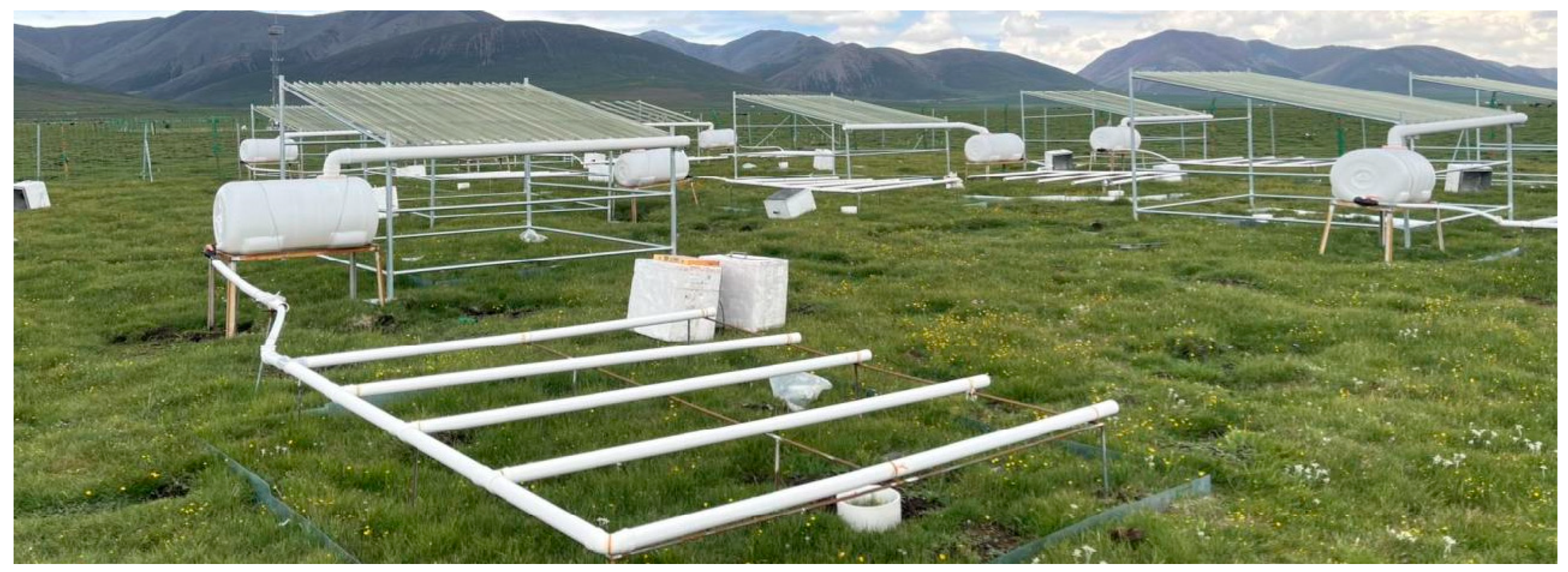
2.2.2. Simulation of Precipitation Devices

The precipitation simulation device was applied for a utility model patent. Using the principle of height difference to achieve automatic precipitation, rainfall reduction treatment for the translucent PC pipe rain collection, covering 75% of the unit area to collect rainwater in the lying box, and rainfall increase treatment for the PVC pipe with uniformly drilled walls, the collected rainwater will evenly be sprinkled in the rainfall increase sample field (Figure 2).

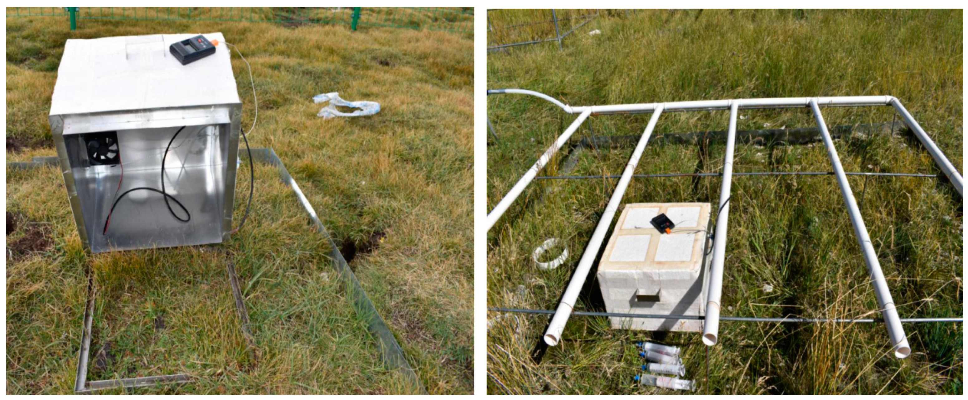
2.2.3. Measurement of GHGs

Field in situ observations of greenhouse gas (CO₂, CH₄, and N₂O) fluxes in the wetlands were conducted from May to September 2020 and 2021. The gas fluxes were measured by static chamber-gas chromatography, with a small fan installed inside the chamber to mix the gases inside the chamber. Each sampling is fixed at 11:00 a.m. and 3:00 p.m. to collect the gas, with sampling at 0, 15, and 30 min after the closed static chamber sampling. A 100 mL medical syringe was connected to a three-way valve outside the chamber to extract the gas while recording the temperature inside the chamber, the soil moisture, and the soil temperature (Figure 3). A total of 2 (2 years) × 2 (2 time points) × 3 (3 time periods) × 3 (3 treatments) × 3 (3 sets of replicates) × 8 (8 dates) = 864 gas samples, and 150 soil samples were collected. It is noteworthy that the CO₂ efflux in this case was a reflection of the ecosystem respiration, since the plant community within the stainless-steel ring was undisturbed and not exposed to light during the flux measurements.

The CO₂, CH₄, and N₂O gas concentrations were measured using an Agilent 7890B gas chromatograph (Agilent Technologies, Santa Clara, CA, USA) Country of equipment (China). All gas samples were measured within 24 h after sampling. The CO₂, CH₄, and N₂O concentrations were measured by gas chromatography. The CO₂ detector is a thermal conductivity detector (TCD). The chromatographic column and sample were HP-5.30 m × 0.32 mm × 0.25 µm (19091J.413), with a flow rate of 6.5 mL·min⁻¹ in a constant flow mode, a packed column inlet temperature of 250 °C, a detector temperature of 300 °C, and a carrier gas of hydrogen. The CH₄ detector was a hydrogen flame ionization detector (FID). The chromatographic column and sample were HP-5.30 m × 0.32 mm × 0.25 µm (19091J.413). The flow rate was 6.5 mL·min⁻¹. The mode was constant flow. The temperature of the packed column inlet was 250 °C. The detector temperature was 300 °C, and the carrier gas was nitrogen. The N₂O detector was a 63Ni electron capture detector (ECD). The chromatographic column and sample were HP-5.30 m × 0.32 mm × 0.25 µm (19091J.413). The flow rate was 6.5 mL·min⁻¹. The mode was constant flow. The temperature of the packed column inlet was 200 °C. The detector temperature was 300 °C, and the carrier gas was argon methane [40].

The equation for wetland greenhouse gas emission fluxes is as follows [41]:

$$F=\rho \times {\displaystyle \frac{V}{A}}\times {\displaystyle \frac{P}{P_0}}\times {\displaystyle \frac{T_0}{T}}\times {\displaystyle \frac{d{C}_t}{dt}}$$

where F is the flux rate (mg·m⁻²·h⁻¹); ρ is the density at standard conditions (g·L⁻¹); V is the chamber volume (m³); A is the chamber base area (m²); P is the air pressure (hpa); P₀ is the standard air pressure (hpa); T₀ is the standard temperature (K); T is the air temperature (K); and dC_t/dt is the rate of change of the gas concentration.

The estimation of the total greenhouse gas emissions is as follows [42]:

$$M={\displaystyle \sum (F_{i+1}+F_i)}/2\times (t_{i+1}-t_i)\times 24\times {10}^{-2}$$

where M is the cumulative flux of detected target gases (kg·hm⁻²); F_i and F_i+1 represent the gas fluxes of the i-th and i + 1-th sampling, respectively (μg·m⁻²·h⁻¹ or mg·m⁻²·h⁻¹); t_i and t_i+1 represent the i-th and i + 1-th sampling dates, respectively; and 10⁻² is the unit conversion factor.

The global warming potential (GWP) is the relative ability to evaluate the impact of different greenhouse gases in the atmosphere on climate change and is calculated as follows [43]:

$$GWP=F_{C{O}_2}+F_{C{H}_4}\times 25+F_{N_{2}O}\times 298$$

where GWP is the global warming potential (t·hm⁻²); FCO₂, FCH₄ and FN₂O indicate the cumulative emission fluxes of different greenhouse gases during the observation period (t·hm⁻²); and 25 and 298 are based on the GWP multipliers of CH₄ and N₂O relative to CO₂ on a 100-year time scale, respectively.

2.2.4. Determination of Soil Physicochemical Properties and Vegetation Characteristics

The soil temperature and soil moisture of 0~10 cm were collected at the same time as a gas collection for the corresponding time period, and a soil auger of 4.2 cm in diameter was used to collect the 0~10 and 10~20 cm soil. The soil temperature was measured using a soil thermometer (TZS-2X, Top Yunong Company, Zhejiang, China), with an accuracy of 0.01 °C, and a soil moisture meter (JK-100F, JIEKESI, Jiangsu, China), with 0.1% accuracy; the soil total nitrogen and total carbon were measured using an ECS4024 elemental analyzer (NC Technologies S.r.l., Bussero, Italy). The soil pH was measured using a PHS-25 instrument (Lei Magnetic Company, Shanghai, China), and soil conductivity was measured using a DDS-307 instrument (Lei Magnetic Company, Shanghai, China).

To calculate the vegetation characteristics, the following equation was used:

$$P_i=(C+D+H)/3$$

where P_i is the proportion of the number of individuals of the i-th species to the number of individuals of all species; C is the relative vegetation cover; D is the relative density of the vegetation; and H is the relative height of the vegetation.

The formula for calculating the indicators of vegetation diversity is as follows:

Simpson’s diversity index: $C=1-{\displaystyle \sum _i^S{P}_i^2}$

$$\mathrm{Shannon}–\mathrm{Wiener}’\mathrm{s} \mathrm{index}: H^{\prime }=-{\displaystyle \sum P_{i}In{P}_i}$$

$$\mathrm{Species} \mathrm{evenness}: J=H^{\prime }/InS$$

where S is the total number of species in each subsample site.

2.2.5. Analyzing and Processing Data

Data were analyzed using SPSS 21.0 (SPSS, Chicago, IL, USA), and the relationship between the CO₂, CH₄, and N₂O fluxes and the soil physicochemical properties was analyzed using a linear fit. The gases between the different precipitation treatments and each physicochemical factor were reduced using a one-way ANOVA of variance (LSD) test. The data descriptions were plotted using the Origin 2021 software.

3. Analysis and Results

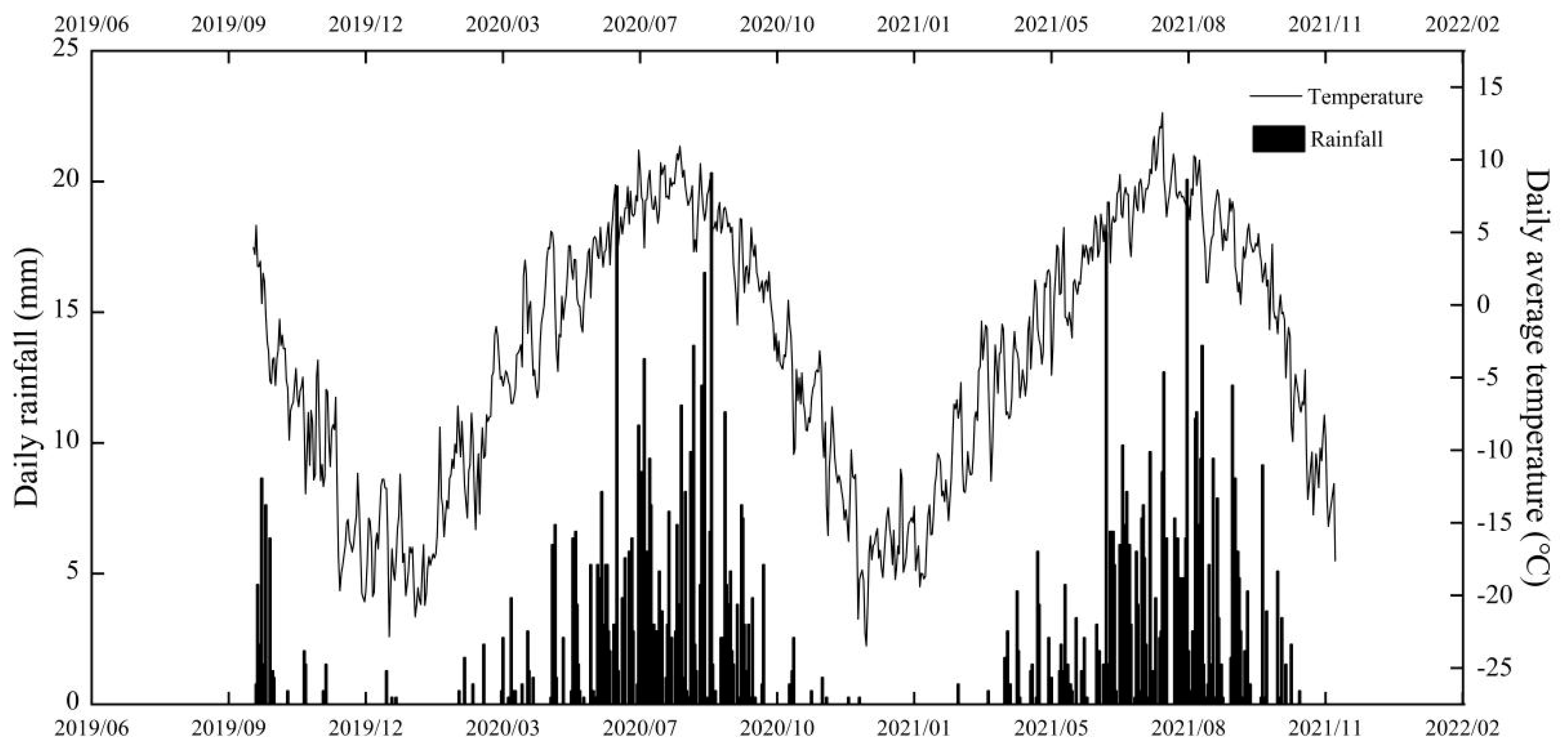
3.1. Environmental Conditions

During the 2020 growing season, the precipitation simulator did not cause any significant change in soil moisture in the IP sample plot, but it reduced the soil moisture in the DP sample plot by 4.72%. While the soil temperature decreased by 0.3 °C in the IP sample plot, it increased by 0.3 °C in the DP sample plot (Figure 4).

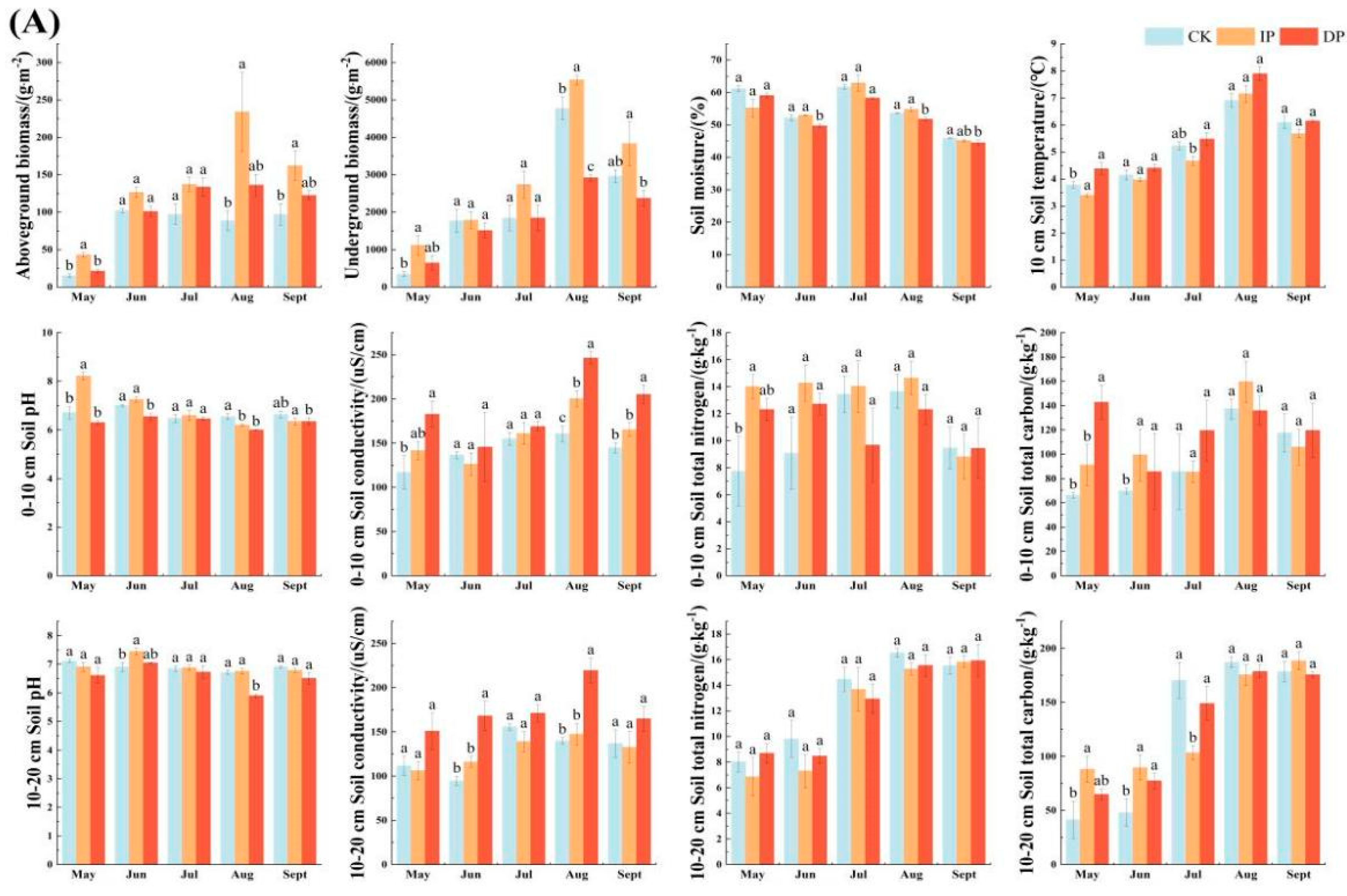
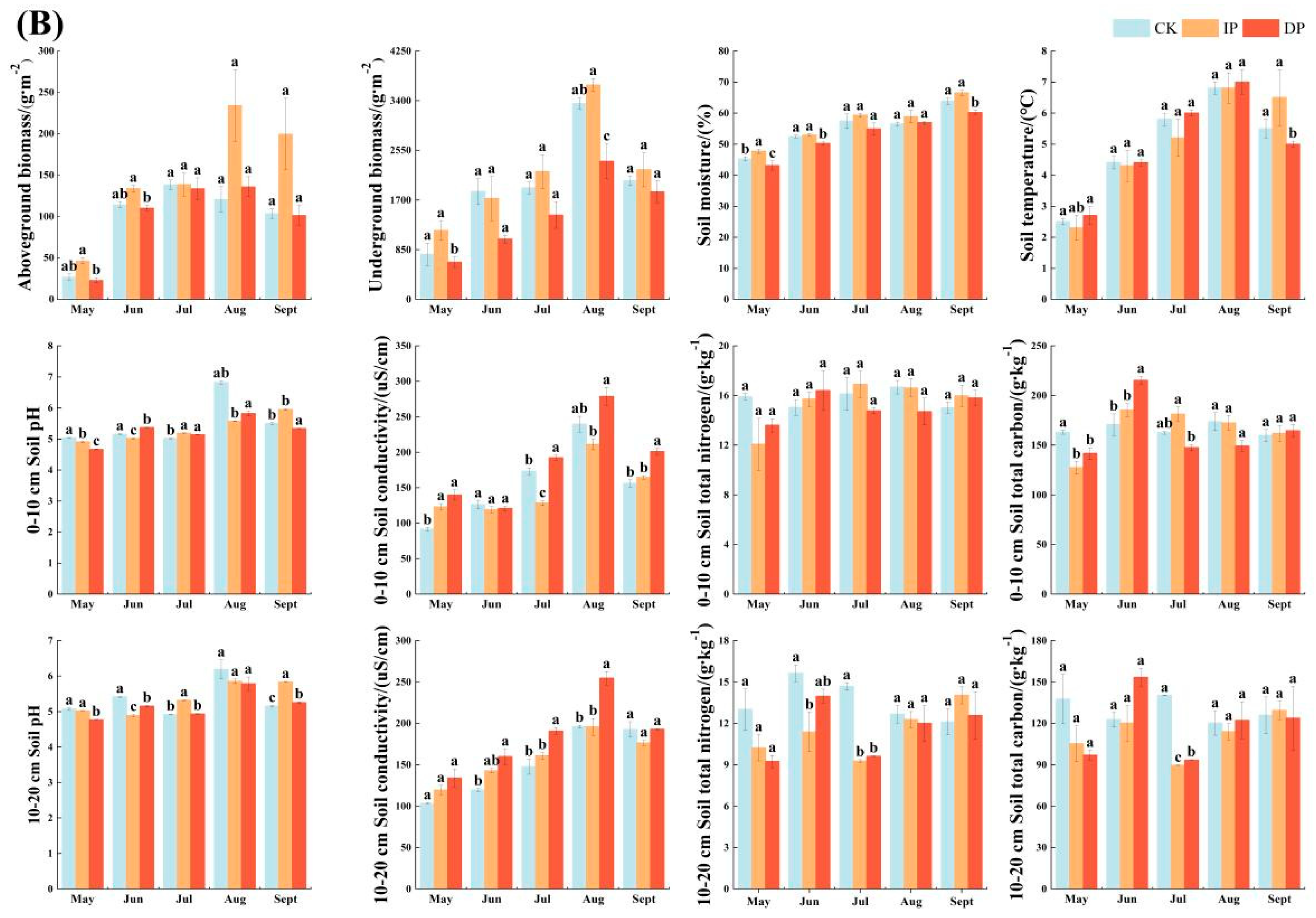
3.2. Characteristics of Vegetation and Soil

The variations in precipitation had a significant impact on the vegetation characteristics, including height, coverage, aboveground biomass, Simpson’s index, and quadrat biomass. In 2020, the aboveground biomass of the quadrat increased significantly with the higher precipitation levels. Furthermore, the vegetation coverage exhibited consistent patterns across different precipitation treatments in 2021 (

Table 1. Vegetation characteristics.

2020	Site	Height (cm)	Coverage (%)	AGB (g·m−2)	Simpson’s index	Species evenness	Shannon–Wiener’s index
	CK	9.00	84.00	80.11	0.022	0.322	0.670
	IP	14.45	90.00	140.69	0.012	0.369	0.012
	DP	6.6	80.00	102.99	0.011	0.352	0.011
2021	Site	Height (cm)	Coverage (%)	AGB (g·m−2)	Simpson index	Species evenness	Shannon–Wiener index
	CK	12.30	86.00	120.67	0.020	0.368	0.766
	IP	13.66	92.50	234.18	0.019	0.379	0.079
	DP	10.54	85.30	136.15	0.023	0.307	0.064

).

3.3. Change in CO₂ Fluxes During the Growing Season Under Simulated Precipitation

The CO₂ flux under all treatments at 11 a.m. during the 2020 growing season in the alpine river source wetland under simulated extreme precipitation peaked in July, increased from May to June, and decreased from August to September. The fluctuation of CO₂ flux was more pronounced at 15 p.m. compared to 11 a.m. From the mean value of the entire growing season, the CO₂ fluxes in all treatments exhibited a “source” state when averaged over the whole growing season (Figure 5). Overall, the CO₂ flux during the 2021 growing season showed a declining trend compared to that of 2020, reaching its maximum in July and August. In 2021, the CK treatment decreased by 54.8% compared to 2020; the IP treatment decreased by 65.1%, and the DP treatment decreased by 52.9%. There were significant differences among all treatments (p < 0.05) (

Table 2. One-way ANOVA analysis of CO₂ flux between months under each treatment during the growing season (means ± SD, n = 15).

2020	Month	CK	IP	DP
	May	23.42 ± 7.65a	16.00 ± 6.30a	20.80 ± 4.12a
	Jun	125.46 ± 14.11a	71.83 ± 6.49ab	50.30 ± 22.97b
	Jul	182.03 ± 15.06a	130.45 ± 34.97a	189.58 ± 47.02a
	Aug	14.36 ± 7.84b	43.68 ± 6.80ab	69.21 ± 17.57a
	Sep	45.59 ± 13.91a	40.91 ± 16.02a	7.81 ± 5.23a
2021	Month	CK	IP	DP
	May	15.30 ± 8.19a	19.88 ± 6.74a	3.98 ± 11.60a
	Jun	37.23 ± 9.97a	15.36 ± 5.66a	47.92 ± 15.57a
	Jul	72.93 ± 15.17a	28.38 ± 8.32b	60.30 ± 14.85ab
	Aug	34.05 ± 12.67a	36.29 ± 17.90a	8.93 ± 10.64a
	Sep	58.75 ± 11.92a	31.38 ± 7.78a	39.71 ± 7.25a

Different lowercase letters represent significant differences (p < 0.05) between the treatments.

). These results indicate that during the growing season of 2020, the CO₂ flux under the IP treatment increased by 27.1% compared to the CK control group, while it increased by 25.5% under the DP treatment compared with the CK control group; however, the CO₂ flux under the IP treatment was lower than the DP flux by 22.6%.

During the growing season of 2021, the CO₂ flux under the IP treatment decreased by 43.7% compared to the CK control group, while it decreased by 22.2% under the DP treatment compared with the CK control group; however, the CO₂ flux under the IP treatment was lower than the DP flux by 27.6%. Soil moisture in river source wetlands under long-term precipitation treatments was not found to be the main factor affecting the CO₂ flux.

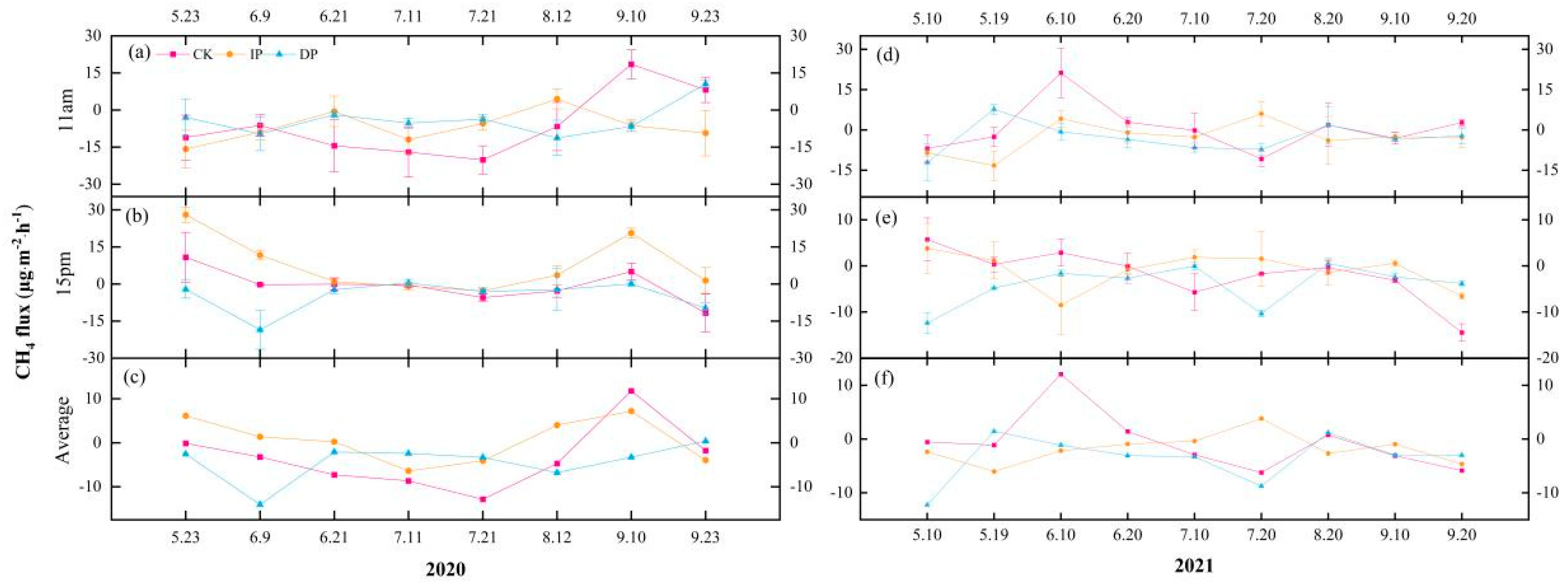
3.4. Change in CH₄ Fluxes During the Growing Season Under Simulated Precipitation

The wetland functions as an intermittent CH₄ source or sink during the growing season: emissions are highly dynamic in early summer (May–June), become stable during the peak growing season (late June–mid-August), and return to high variability post mid-August (Figure 6). In 2020, CH₄ fluxes of >0.041 µg·m⁻²·h⁻¹ were detected several times at the end of the growing season (10 September, 23 September). The 15 p.m. CH₄ flux was significantly higher than the 11 a.m. CH₄ flux under IP processing, but the opposite was true under DP processing. The CH₄ flux under the IP treatment is 84.1% higher than that under the DP treatment.

In the 2021 growing season, the wetland quadrat under all treatments showed a CH₄ “sink” state, and the emission state was only concentrated from the end of May to the middle of June; the absorption capacity of the DP treatment was 48.72% higher than that of the IP treatment. Precipitation change is not the main factor affecting CH₄ emission in the river source wetland (

Table 3. One-way ANOVA analysis of CH₄ flux between months under each treatment during the growing season (means ± SD, n = 15).

2020	Month	CK	IP	DP
	May	−0.13 ± 3.95a	6.12 ± 22.20a	−2.54 ± 6.73a
	Jun	−5.24 ± 2.43a	0.79 ± 4.75a	−8.07 ± 3.79a
	Jul	−10.73 ± 7.38a	−5.25 ± 2.95a	−2.87 ± 1.23a
	Aug	−5.06 ± 7.49a	4.84 ± 8.07a	−8.72 ± 6.22a
	Sep	5.00 ± 3.08a	1.50 ± 4.44a	−1.43 ± 1.17a
2021	Month	CK	IP	DP
	May	−0.83 ± 2.50a	−4.19 ± 3.11a	−5.39 ± 4.43a
	Jun	6.74 ± 3.69a	−1.54 ± 8.73b	−2.10 ± 4.30b
	Jul	−4.57 ± 3.69a	1.72 ± 2.20a	−6.03 ± 1.37a
	Aug	0.76 ± 4.50a	−2.67 ± 9.87a	1.19 ± 3.79a
	Sep	−4.47 ± 2.05a	−2.79 ± 1.35a	−2.98 ± 0.8a

Different lowercase letters represent significant differences (p < 0.05) between the treatments.

).

3.5. Change in N₂O Fluxes During the Growing Season Under Simulated Precipitation

There was no significant seasonal variation observed in N₂O flux across all simulated precipitation treatments (Figure 7). In the growing season of 2020, all three treatments were characterized as “sources” of N₂O flux. On 12 August, at 11 a.m., the IP and DP treatments both showed a peak N₂O flux of 20.437 µg·m⁻²·h⁻¹ and 10.341 µg·m⁻²·h⁻¹, respectively. However, at 15 p.m., the IP treatment decreased to −1.581 µg·m⁻²·h⁻¹, while the DP treatment decreased to −6.661 µg·m⁻²·h⁻¹. This may be due to the fact that the sampling point began raining at 12 pm on the observation day and stopped raining at 15:30 pm. The N₂O flux may have transitioned from a “source” to a “sink” due to the pulse effect. Compared to the CK treatment, the N₂O flux in the IP treatment increased by 81.9%, and the N₂O flux in the DP treatment increased by 67.9%. The N₂O flux in the IP treatment was 43.8% higher than that in the DP treatment.

In the growing season of 2021, only the IP treatment exhibited a “weak sink” status. At 11 a.m., under the CK condition, it was shown as a “weak sink” of N₂O. At 15 p.m., as the soil temperature rose, the wetland began to emit N₂O gas. Throughout the growing season observation, it was indicated that the N₂O flux under the DP treatment increased exponentially, while the N₂O flux in the IP treatment was 552.1% lower than that in the DP treatment. Extremely reduced precipitation will significantly affect the emission of N₂O (

Table 4. One-way ANOVA analysis of N₂O flux between months under each treatment during the growing season (means ± SD, n = 15).

2020	Month	CK	IP	DP
	May	−3.38 ± 0.75a	1.76 ± 1.44a	0.58 ± 2.10a
	Jun	2.15 ± 2.37a	−0.62 ± 1.27a	0.29 ± 3.60a
	Jul	−0.83 ± 1.08a	0.96 ± 1.60a	2.67 ± 0.88a
	Aug	1.03 ± 0.54a	10.00 ± 3.98a	2.71 ± 6.77a
	Sep	1.64 ± 0.72a	3.86 ± 2.63a	1.33 ± 1.18a
2021	Month	CK	IP	DP
	May	0.59 ± 1.16a	4.11 ± 4.23a	3.10 ± 4.97a
	Jun	0.24 ± 0.94a	0.82 ± 0.62a	1.27 ± 1.04a
	Jul	−0.35 ± 0.55a	−4.59 ± 4.02a	0.73 ± 0.68a
	Aug	−4.23 ± 2.18a	−1.90 ± 0.66a	−0.14 ± 1.37a
	Sep	−0.20 ± 0.57a	−0.01 ± 0.26a	−0.58 ± 0.26

Different lowercase letters represent significant differences (p < 0.05) between the treatments.

).

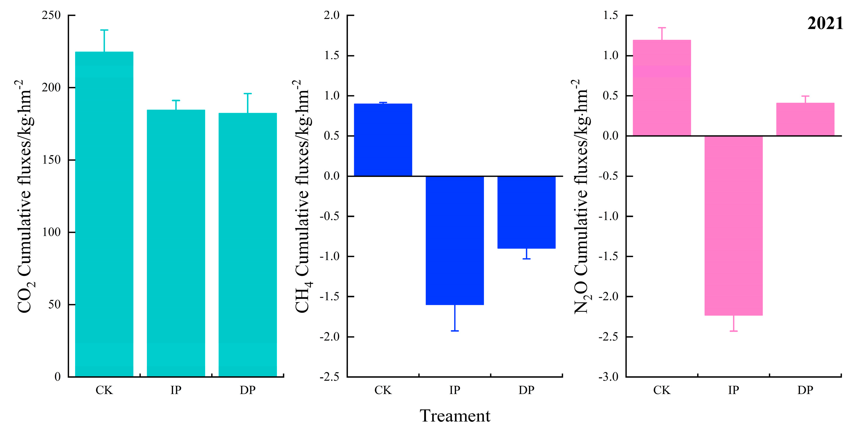
3.6. Cumulative Greenhouse Gas Emissions and Global Warming Potential (GWP) of the Wayan Mountain River Source Wetlands

In 2020, the cumulative CO₂ flux under a precipitation treatment was 284.76 (CK), 258.38 (IP), and 259.61 kg·hm⁻², with contributions to global warming potential of 100.66%, 99.87%, and 100.76%, respectively. In 2021, it was 224.68 (CK), 184.46 (IP), and 182.32 kg·hm⁻², with contributions of 99.08%, 102.12%, and 100.27%, respectively (Figure 8). The contribution rate of CO₂ flux to the global warming potential under the precipitation treatment was lower than that in natural conditions, indicating that the inhibition of the greenhouse effect by an extreme precipitation increase in the region is greater than that by an extreme precipitation decrease, so the “warm and moisturizing” of the Qinghai–Tibet Plateau may play a positive feedback role on CO₂ emissions in the river source wetland. The cumulative CH₄ flux under the precipitation treatment was −2.6 (CK), −0.7 (IP), and −3.0 kg·hm⁻², with contributions to the global warming potential of −0.92%, −0.27%, and 0.40%, respectively. In 2021, it was 0.9 (CK), −1.6 (IP), and −0.9 kg·hm⁻², with contributions of 0.40%, −0.89%, and −0.49%, respectively. The CH₄ flux in the Wafangshan River source wetland was in a “sink” state both in natural conditions and under the precipitation treatment, and the increase in water did not cause an increase in CH₄ flux emissions, but the CH₄ flux went from a “sink” to a “weak sink”, indicating that the increase in water, to some extent, inhibited the absorption of methane. The cumulative N₂O flux under the precipitation treatment was as follows: 0.73 (CK), 1.03 (IP), and 1.04 (DP) kg·hm⁻², with the respective contributions to the global warming potential being 0.26%, 0.40%, and 0.40%. In 2021, the cumulative N₂O flux was as follows: 1.19 (CK), −2.23 (IP), and 0.41 (DP) kg·hm⁻², with respective contributions of 0.52%, −1.23%, and 0.23%. Extreme water reduction caused the wetland soil to become acidic, and the acidic soil, to some extent, promoted the emission of N₂O.

3.7. Effect of Extreme Precipitation Variability on Greenhouse Gas Fluxes in Alpine River Source Wetlands

Extreme precipitation changes altered the soil moisture and temperature in the alpine river source wetland, thereby changing the soil physical and chemical properties and biomass, which affected greenhouse gas fluxes, consistent with the results of most rainwater treatment experiments [44,45,46]. During the two growing seasons, the soil moisture in the IP treatment was 1.21% higher than that in the CK group, while the soil temperature decreased by 0.28 °C. In contrast, the soil moisture in the DP treatment decreased by 2.44%, while the soil temperature increased by 0.20 °C. This contrasting result is understandable for the wetland ecosystem, as the solar radiation is stronger in the high-altitude region, and the high moisture soil will cause a certain degree of soil temperature decrease.

The IP treatment increased the aboveground biomass of the high-altitude wetland in the growing season by 62.5%, and the biomass of the 0–10 cm soil layer by 19.5% (Figure 9). Therefore, the autotrophic respiration of plants increased with the increase in precipitation. The simulated extreme precipitation treatment did not lead to a further rise in the CO₂ flux, which may be due to the fact that the wetland soil pores were completely filled with water after extreme precipitation, so that soil respiration could not be fully released. The IP treatment reduced the total soil carbon by 6.8%, and the DP treatment increased it by 11.5%, but the Re flux did not react. This may be due to the fact that temperature is the main limiting factor for high-altitude wetland ecosystems. Therefore, it can be inferred that the extreme increase in precipitation does not stimulate the CO₂ flux in the wetland but rather inhibits it.

In the alpine-cold source wetland with a two-year growing season, the CH₄ flux naturally acts as a “sink” (−1.98 µg·m⁻²·h⁻¹). After adding rainwater, the wetland’s CH₄ flux “sink” capacity decreases (−0.62 µg·m⁻²·h⁻¹), while after rainfall reduction, the CH₄ absorption capacity improves by 49.2% compared to the CK group (−3.89 µg·m⁻²·h⁻¹). This indicates that after an extreme increase in precipitation in alpine-cold source wetlands, a certain amount of CH₄ is released, resulting in a state of emission source. Additionally, during monitoring on July 11 and September 23, it was found that the CH₄ flux absorption rates of the IP treatment (−6.40, −3.94 µg·m⁻²·h⁻¹) were higher than those of the CK control group (−0.30, −1.78 µg·m⁻²·h⁻¹). It can be predicted that extreme precipitation events caused by global warming will either increase or decrease the CH₄ flux. The impact of precipitation changes on CH₄ fluxes in wetland ecosystems involves complex mechanisms characterized by counteracting effects among multiple factors. Although increased extreme precipitation during the growing season elevates the soil moisture (theoretically favoring methanogen activity while inhibiting CH₄ diffusion), observational studies indicate no significant net effect on CH₄ fluxes. This phenomenon can be explained by the following coupled mechanisms: Firstly, enhanced precipitation suppresses CH₄ emissions through dual pathways: (1) The stimulated growth of belowground plant biomass increases the root respiration-driven oxygen consumption, reducing oxygen availability in the anaerobic zone and directly inhibiting the aerobic metabolism of methanotrophs, thereby weakening the CH₄ oxidation rates. (2) Concurrent cooling effects from precipitation lower the soil temperature, reducing the microbial enzyme activity and, thus, constraining the metabolic intensity of both methanogens and methanotrophs. Secondly, while increased precipitation raises soil water content and impedes CH₄ diffusion, this effect is partially offset by the aforementioned biogeochemical suppression mechanisms. Notably, oxygen competition plays a critical role—increased root respiration competes with methanotrophs for limited oxygen, significantly reducing the oxidation and uptake of atmospheric CH₄ in the surface soil.

Wetlands are commonly regarded as a “sink” for N₂O, with N₂O fluxes controlled by nitrification and denitrification processes. The absorption of N₂O occurs during rainy days when N₂O, consumed by denitrifying bacteria, moves downwards and is absorbed by the soil moisture. This experimental design did not involve sampling on specific rainy days; instead, a precipitation simulation setup was used as part of a long-term effect study to observe changes in greenhouse gases in wetlands following extended periods of extreme precipitation. Consequently, in our study, the N₂O fluxes under the intensified precipitation (IP) treatment were approximately 178.4% and 137.8% higher than those in the control (CK) group and the decreased precipitation (DP) treatment, respectively. The N₂O fluxes were observed in an absorption state (IP: −3.45, −4.22 µg·m⁻²·h⁻¹) only on 21 June 2020 and 10 July 2021. The IP treatment increased the total nitrogen content by 18.9% in the 10 cm soil layer, while there was no significant change in the 20 cm soil layer. In alpine river source wetlands, N₂O switched from a weak source to a source under conditions of extremely increased precipitation and remained a source even under extremely decreased precipitation. Both scenarios exhibited stronger N₂O emission capabilities compared to the CK group, indicating that N₂O fluxes are sensitive to changes in moisture under both extreme conditions.

3.8. Comparison of Greenhouse Gases in Alpine Wetlands with Those in Other Types of Wetland

The difference between the greenhouse gas fluxes of the river source wetlands in Wayan Mountain and several other typical wetlands is obvious, especially the greenhouse gas emissions after a rainwater treatment (

Table 5. Greenhouse gas emissions from different types of wetland ecosystems.

Wetland Type	CO2 (mg·m−2·h−1)	CH4 (mg·m−2·h−1)	N2O (µg·m−2·h−1)	Remark
Coastal Wetland	98.01–1359.25 (Hu et al., 2005) [46]	0.044 (Xu et al., 2015) [50]	5.92–180.38 (Zhu et al., 2013) [46]	The Growing Season
		0.079 (Wang et al., 2010) [51]	2.02–20.84 (Yang et al., 2013) [52]
	231.6–557.1 (Yang et al., 2013) [52]
Artificial wetland	0.02–17.4 (Sille Teiter, 2005) [53]	0.001–0.265 (SilleTeiter, 2005) [53]	−0.0004–0.058 (Sille Teiter, 2005) [53]	Year round
	431.92 (Xu, 2020) [50]	0.017 (Xu, 2020) [50]	0.100 (Xu, 2020) [50]	Non-growing season
Marsh wetland	1.5–238.4 (Li, 2019) [17]	−0.019–0.011 (Li, 2019) [17]	27.1 (Li, 2019) [17]	Indoor cultivation
		−0.00584–0.00926 (Ren, 2020) [54]		Year round
		0.0033 (Song, 2006) [55]	13.31 (Song, 2006) [55]	The Growing Season
Tidal flats wetland	−101.93 (Hu, 2014) [56]	0.00746 (Hu, 2014) [56]	2.22 (Hu, 2014) [56]	Year round
Peat wetland	203.22 (Wang, 2010) [51]	2.43 (Wang, 2010) [51]	20 (Wang, 2010) [51]	The Growing Season

). This conclusion is unexpected because the tidal flats wetland is water-rich or even supersaturated, while the river source wetland appears to be a “sink” when precipitation is extremely reduced, probably because this experiment did not collect gas in the winter and ignored the ecological respiration emission flux of the wetland during the non-growing season. It was found that the CH₄ fluxes in each type of wetland were unstable, with marsh wetlands, artificial wetlands, and coastal wetlands all showing a “sink” of CH₄ fluxes when there was sufficient water. The state of the N₂O flux is the most unstable among all wetland types, and it is not clear how it changes, and the range of variation is wide. For example, N₂O fluxes in artificial wetlands can change from −0.49 µg·m⁻²·h⁻¹ to 0.11 µg·m⁻²·h⁻¹ directly, but the average values of N₂O fluxes in all types of wetlands throughout the year or the growing season are all shown as a “source”. The emissions are much greater than the absorption. The pattern of seasonal changes in N₂O emissions in this experiment is not obvious, but the average values are all shown as a “source”. In summary, the emission fluxes of respiration from the Wayan Mountain River source wetland ecosystem throughout the growing season are broadly convergent compared to all types of wetlands. As a major player in the global carbon cycle, wetlands can act as both a source and a sink of greenhouse gases [47], and their status depends on the temperature, moisture, precipitation, wind speed, soil physicochemical properties, microbial species, numbers, and activity of the entire wetland ecosystem [48,49], so the respiration of wetland ecosystems cannot be considered from purely physicochemical properties or microbial; it is necessary to consider all factors together.

3.9. Test Interference Factors

Some possible disturbing factors exist in this experiment. Firstly, grazing is a point that cannot be neglected in the Qinghai Lake basin area, and this experiment isolated the sample site from livestock by fencing. Guo Xiaowei et al. [57] observed the growing season fluxes of grazed alpine meadows of the Qinghai–Tibet Plateau and found that the CO₂ fluxes of lightly degraded meadows were 400.1 ± 52.1 mg·m⁻²·h⁻¹ and 521.2 ± 113.8 mg·m⁻²·h⁻¹ for heavily degraded meadows. The CH₄ flux in the lightly degraded meadow was −37.8 ± 11.6 µg·m⁻²·h⁻¹ and 56.7 ± 19.3 µg·m⁻²·h⁻¹ in the heavily degraded meadow; the N₂O flux in the lightly degraded meadow was 35.17 ± 7.5 µg·m⁻²·h⁻¹ and 87.07 ± 8.9 µg·m⁻²·h⁻¹ in the heavily degraded meadow. Therefore, the effect of grazing factors on greenhouse gas flux emissions cannot be ignored.

Secondly, rainwater collection through transparent PC tubes in this experiment cannot be avoided by blocking part of the solar radiation. Jia Lei et al. [57] found that CO₂ flux was significantly negatively correlated with solar radiation (p < 0.01), and the average photosynthetic effective radiation in the growing season in the experimental area was 411.10 V/m², so the CO₂ flux may have been overestimated to some extent.

Finally, the time period of 11 a.m. to 15 p.m. was chosen as the sampling time in this experiment because the test area is in an unoccupied area with a harsh environment, and the collection of gas samples, as well as plant and soil samples, was performed by one person; thus, the data collection could not be completed at multiple time points, so the sampling time point was used as the sampling time point according to former researchers and other researchers for the occurrence of daily average values in the watershed during the growing season.

The experimental sample in the Wayan Mountain River source wetland was treated for 4 years (2018–now) to produce more meaningful results than the short-term treatment.

4. Conclusions

The main objective of this study is to investigate the effects of increased extreme precipitation events due to climate warming on greenhouse gas fluxes in alpine river source wetlands. Combined with the results of studies on the effect of extreme precipitation events on greenhouse gases in wetlands, the extreme increase in precipitation has an effect (positive and negative) on greenhouse gases. The results of this study show that extreme increases and decreases in precipitation have a suppressive effect on CO₂ fluxes. Extreme increases in precipitation have a significant promoting effect on CH₄ fluxes, while extreme decreases in precipitation also play a suppressive role. For N₂O fluxes, extreme increases in precipitation significantly promote their emissions, and extreme decreases in precipitation also significantly promote them, but the promoting effect is only 43% of that of increased precipitation.

Therefore, neither extreme increases nor decreases in precipitation contribute significantly to the carbon source of alpine riverine wetlands, but the contribution to CH₄ and N₂O fluxes cannot be ignored. Wetland ecosystems are inherently carbon reservoirs, with a higher content than other types of ecosystems, so the response of wetlands to climate change cannot be ignored.

References

1. Zhao, X.Q.; Huang, J.; Lu, J.; Sun, Y. Study on the influence of soil microbial community on the long-term heavy metal pollution of different land use types and depthlayers in mine. China. Ecotoxicol. Environ. Saf. 2019, 170, 218–226. [Google Scholar] [CrossRef]
2. Stocker, T.F.; Qin, D.; Plattner, G.-K.; Tignor, M.; Allen, S.K.; Boschung, J.; Nauels, A.; Xia, Y.; Bex, V.; Midgley, P.M. (Eds.) Climate Change 2013: The Physical Science Basis. In Contribution of Working Group I to the Fifth Assessment Report of IPCC the Intergovernmental Panel on Climate Change; Cambridge University Press: Cambridge, UK; New York, NY, USA, 2014. [Google Scholar]
3. You, Q.; Kang, S.; Aguilar, E.; Pepin, N.; Flügel, W.-A.; Yan, Y.; Xu, Y.; Zhang, Y. Changes in daily climate extremes in China and their connection to the large scale atmospheric circulation during 1961–2003. Clim. Dyn. 2011, 36, 2399–2417. [Google Scholar] [CrossRef]
4. Rahimi, M.; Mohammadian, N.; Vanashi, A.R.; Whan, K. Trends in Indices of Extreme Temperature and Precipitation in Iran over the Period 1960–2014. Open J. Ecol. 2018, 8, 396. [Google Scholar] [CrossRef]
5. Feng, G. Research on Detection, Diagnosis and Predictability of Extreme Climate Events; Science Press: Beijing, China, 2012. [Google Scholar]
6. Wang, X. Characteristics of Soil N2O Emission and Its Main Influencing Factors During the Freeze-Thaw Period of Non-Growing Season of Typical Grassland in Temperate Zone. Ph.D. Thesis, Chang’an University, Xi’an, China, 2020. [Google Scholar]
7. Pachauri, R.K.; Allen, M.R.; Barros, V.R.; Broome, J.; Cramer, W.; Christ, R.; Church, J.A.; Clarke, L.; Dahe, Q.D.; Dasqupta, P.; et al. Climate Change 2014 Synthesis Report; Contribution of working groups I, II, and III to the fifth assessment report of the Intergovernmental Panel on Climate Change. Synthesis report; Environ. Policy Collect.; Intergovernmental Panel on Climate Change: Geneva, Switzerland, 2014; 151p. [Google Scholar]
8. Wang, Y.; Lu, J. A review on litter decomposition and its impact factor in terrestrial ecosystems. Bull. Sci. Technol. 2017, 33, 1–10. [Google Scholar]
9. Yang, K.; Hui, W.U.; Qin, J.; Lin, C.; Tang, W.; Chen, Y. Recent climate changes overthe Tibetan Plateau and their impacts on energy and water cycle: A review. Glob. Planet. Change 2014, 112, 79–91. [Google Scholar] [CrossRef]
10. Xu, Y.L.; Xue, F.; Lin, Y.H. Changes of surface air temperature and precipitation in China during the 21st century simulated by had CM2 under different greenhouse gas emission scenarios. Clim. Environ. Res. 2003, 8, 209–217. [Google Scholar] [CrossRef]
11. Ofipcc, W.G.I. Climate change; the physical science basis. Contrib. Work. 2013, 43, 866–871. [Google Scholar]
12. Greve, P.; Orlowsky, B.; Mueller, B.; Sheffield, J.; Reichstein, M.; Seneviratne, S.I. Corrigendum: Global assessment of trends in wetting and drying over land. Nat. J. Geosci. 2014, 7, 848. [Google Scholar] [CrossRef]
13. Yang, Z.W. Study on Greenhouse Gas Emission Characteristics and Influencing Factors of Huayanshan River Source Wetland Under Simulated Precipitation. Ph.D. Thesis, Qinghai Normal University, Qinghai, China, 2022. [Google Scholar]
14. Wang, H.X. CH4 Flux Characteristics of Different Grazing Methods of Artificial Grassland in Semi-Arid Area of Inner Mongolia. Ph.D. Thesis, Inner Mongolia University, Hohhot, China, 2014. [Google Scholar]
15. Fang, H.; Cheng, S.; Yu, G.; Cooch, J.; Wang, Y.; Xu, M.; Li, L.; Dang, X.; Li, Y. Low-level nitrogen deposition significantly inhibits methane uptake from an alpine meadow soil on the Qinghai-Tibetan Plateau. Geoderma 2014, 213, 444–452. [Google Scholar] [CrossRef]
16. Tang, S.; Wang, C.; Wilkes, A.; Zhou, P.; Jiang, Y.; Han, G.; Zhao, M.; Huang, D.; Schönbach, P. Contribution of grazing to soil atmosphere CH4 exchange during the growing season in a continental steppe. Atmos. Environ. 2013, 67, 170–176. [Google Scholar] [CrossRef]
17. Li, Y.; Huang, J.; Yue, H.; Liu, C.; Jiang, C.; Zheng, X. Effects of precipitation and soil freeze-thaw cycles on greenhouse gas exchanges in a permafrost swamp of the Great Hing an Mountains, China. Agro-Environ. Sci. 2019, 38, 2420–2428. [Google Scholar]
18. McCulley, R.L.; Boutton, T.W.; Archer, S.R. Soil respiration in a subtropical savanna parkland: Response to water additions. Soil Sci. Soc. Am. J. 2007, 71, 820–828. [Google Scholar] [CrossRef]
19. Wu, H.; Lee, X. Short-term effects of rain on soil respiration in two New England forests. Plant Soil 2011, 338, 329–342. [Google Scholar] [CrossRef]
20. Lu, H.; Liu, S.; Wang, H.; Luan, J.; Schindlbacher, A.; Liu, Y.; Wang, Y. Experimental throughfall reduction barely affects soil carbon dynamics in a warm temperate oak forest, Central China. Sci. Rep. 2017, 7, 15099. [Google Scholar] [CrossRef] [PubMed]
21. Wang, D.X.; Ding, W.X.; Wang, Y.Y. Main environmental impact factors of CH4 emission difference between swamp wetlands of Zoige Plateau and Sanjiang Plain. Wetl. Sci. 2003, 1, 63–67. [Google Scholar]
22. Song, C.C.; Yang, W.Y.; Xu, X.F.; Yan, J.; Jin, B. Dynamics and influencing factors of soil CO2 and CH4 emissions in marshland ecosystems. Environ. Sci. 2004, 25, 1–6. [Google Scholar]
23. Bao, Z.Z. Effects of Water Change and Simulated Nitrogen Deposition on Soil CH4, CO2 and N2O Emissions in Alpine Wetlands. Ph.D. Thesis, Xinjiang Agricultural University, Urumqi, China, 2018. [Google Scholar]
24. Wei, H.X.; Zhao, J.X.; Luo, T.X. The effect of pika grazing on Stipa purpurea is amplified by warming but alleviated by increased precipitation in an alpine grassland. Plant Ecol. 2019, 220, 371–381. [Google Scholar] [CrossRef]
25. Gao, Q.Z.; Li, Y.; Xu, H.M.; Wan, Y.F.; Jiangcun, W.Z. Adaptation strategies of climate variability impacts on alpine grassland ecosystems in Tibetan Plateau. J. Mitig. Adapt. Strateg. Glob. Change 2014, 19, 199–209. [Google Scholar] [CrossRef]
26. Zhao, J.X.; Luo, T.X.; Li, R.C.; Wei, H.X.; Li, X.; Du, M.Y.; Tang, Y.H. Precipitation alters temperature effects on ecosystem respiration in Tibetan alpine meadows. Agric. For. Meteorol 2018, 252, 121–129. [Google Scholar] [CrossRef]
27. Tao, Z.; Wang, G.; Yan, Y.; Mao, T.; Chen, X. Grassland types and season-dependent response ofecosystemrespiration to experimental warming in a permafrost region in the Tibetan Plateau. Agric. For. Meteorol. 2017, 247, 271–279. [Google Scholar]
28. Althuizen, I.H.J.; Lee, H.; Sarneel, J.M.; Vandvik, V. Long-term climate regime modulates the impact of short-term climate variability on decomposition in alpine grassland soils. Ecosystems 2018, 21, 1580–1592. [Google Scholar] [CrossRef]
29. Dan, Z.T.Q.; Xu, R.; Wei, X.H.; Wei, D.; Liu, Y.W.; Wang, Y.H. Comparative study on major greenhouse gas fluxes in Namco alpine grassland, alpine meadow and swampy meadow. J. Grassl. 2014, 22, 493–501. [Google Scholar]
30. Han, Y.L.; Yu, D.Y.; Chen, K.L.; Yang, H.Z. Spatial distribution characteristics of temperature and precipitation trends in Qinghai Lake basin from 2000 to 2018. Arid Land Geogr. 2020, 45, 999–1009. [Google Scholar]
31. Chen, H.Y.; Zheng, Q.S.; Li, X.Y.; Ma, G.Q.; Xue, C.K.; Jiang, F. Dynamic change analysis of wetland landscape pattern in Qinghai Lake Basin in the past two decades. China Sci. Technol. Inf. 2022, 84–88+90. [Google Scholar]
32. Qi, Y. Study on Wetland Changes in Qinghai Lake Basin in the Past 20 Years. Ph.D. Thesis, Qinghai Norm. University, Qinghai, China, 2012. [Google Scholar]
33. Zhang, J.; Chen, Y.; Ge, J.; Nie, X. Land use/cover change and land resources management in the lakering area of Qinghai Lake from 1977 to 2010. J. Desert Res. 2013, 33, 1256–1266. [Google Scholar]
34. Wu, H.; Chen, K.; Zhang, L.; Ding, J. Effects of warming on major greenhouse gas fluxes in alpine swamp meadows in Qinghai Lake Basin. Grassl. Turf. 2021, 41, 1–9. [Google Scholar]
35. Yang, Z.; Che, Z.; Liu, F.; Chen, K. Effects of precipitation gradient on diurnal variation of greenhouse gas emissions from wetlands in Qinghai Lake source. Arid Land Res. 2022, 39, 754–766. [Google Scholar]
36. Gao, L.; Zhang, L.; Chen, K.; Mao, Y. Photosynthetically effective radiation characteristics of alpine wetlands in Qinghai Lake Basin. Arid Zone Res. 2018, 35, 50–56. [Google Scholar]
37. Zhang, L.; Gao, L.; Chen, K. Radiation balance and surface albedo variation characteristics of Huayanshan wetland in Qinghai Lake Basin. Glaciol. Geocryol. 2018, 40, 1216–1222. [Google Scholar]
38. Zheng, Z.; Yu, G.; Sun, X.; Cao, G.; Wang, Y.; Du, M.; Li, J.; Li, Y. Comparison of vorticity correlation method and static box/gas chromatography in ecosystem respiration observation. China J. Appl. Ecol. 2008, 19, 290–298. [Google Scholar]
39. Chen, Z.; Jiang, L.; Yang, Z.; Chen, K.; Ma, Y. An Automatic Water Diversion Device for Simulating Precipitation. Patent CN202021447963.3, 2 April 2021. [Google Scholar]
40. Yang, Z.W.; Chen, K.L.; Zhang, L.L.; Jiang, L.; Zuo, D. Response of CO2, CH4 and N2O emission fluxes to simulated precipitation in two different alpine wetland types in Qinghai Lake basin. Ecol. Sci. 2022, 41, 211–219. [Google Scholar]
41. Cao, G.; Xu, X.; Long, R. Methane emissions by alpine plant communities in the Qinghai-Tibet Plateau. Biol. Lett. 2008, 4, 681–684. [Google Scholar] [CrossRef]
42. Wu, X.W.; Zang, S.Y.; Ma, D.L. Greenhouse gas flux of forest soil in permafrost area of Daxing’anling. Acta Geogr. Sin. 2020, 75, 2319–2331. [Google Scholar]
43. Nordhaus, W.D. To tax or not to tax: Alternative approaches to slowing global warming. Rev. Environ. Econ. Policy 2007, 1, 26–44. [Google Scholar] [CrossRef]
44. Chen, X.; Wang, G.; Zhang, T.; Mao, T.; Wei, D.; Hu, Z.; Song, C. Effects of warming and nitrogen fertilization on GHG flux in the permafrost region of an alpine meadow. J. Atmos. Environ. 2017, 157, 111–124. [Google Scholar] [CrossRef]
45. Wei, D.; Ri, X.; Liu, Y.; Wang, Y.; Wang, Y. Three-year study of CO2 efflux and CH4/N2O fluxes at an alpine steppe site on the central Tibetan Plateau and their responses to simulated N deposition. Geoderma 2014, 232–234, 88–96. [Google Scholar] [CrossRef]
46. Hu, Q.W.; Wu, Q.; Li, D.; Cao, G. Comparative study on CH4 release in alpine grassland under different soil moisture content. Chin. J. Ecol. 2005, 24, 118–122. [Google Scholar]
47. White, R.P.; Murray, S.; Rohweder, M. Pilot analysis of global ecosystems: Grassland ecosystems. World Resour. Inst. 2000, 4, 275–287. [Google Scholar]
48. Liu, C.; Holst, J.; Brüggemann, N.; Butterbach-Bahl, K.; Yao, Z.; Yue, J.; Han, S.; Han, X.; Krümmelbein, J.; Horn, R.; et al. Winter-grazing reduces methane uptake by soils of a typical semi-arid steppe in Inner Mongolia, China. Atmos. Environ. 2007, 41, 5948–5958. [Google Scholar] [CrossRef]
49. Hu, H. Greenhouse Gases Fluxes at Yangtze Estuary Phragmites australis Wetland and the Influencing Factors. Master’s Thesis, East China Normal University, Shanghai, China, 2014. [Google Scholar]
50. Xu, X. The Temporal and Spatial Dynamies Ofgreenhouse Gases Emissions and Controlling Factors from Coastal Saline Wetlands in Jiangsu Province, Southeast China. Master’s Thesis, Key Laboratory of Coastal and Island Development of Ministry of Education, Nanjing University, Nanjing, China, 2015. [Google Scholar]
51. Wang, D. Emission fluxes of carbon dioxide, methane and nitrous oxide from peatbog in Zoige Plateau. J. Wetl. Sci. 2010, 8, 220–224. [Google Scholar]
52. Yang, P.; Tong, C. Greenhouse gas flux from forests and wetlands: A review of the effects of disturbance. Acta Ecol. Sin. 2012, 32, 5254–5263. [Google Scholar] [CrossRef]
53. Teiter, S.; Mander, Ü. Emission of N2O, N2, CH4, and CO2 from constructed wetlands for wastewater treatment and from riparian buffer zones. Ecol. Eng. 2005, 25, 528–541. [Google Scholar] [CrossRef]
54. Ren, R. Effects of Extreme Precipitation on Soil CH4 Fluxes in the Songnenmeadow Steppe Under Different Nitrogen Addition and Grazing Treatments. Master’s Thesis, Northeast Normal University, Changchun, China, 2020. [Google Scholar]
55. Song, C.; Wang, Y.Y.; Wang, Y.S.; Zhao, Z.C. Changes of greenhouse gas emissions in freshwater marsh wetlands under the influence of human activities. Sci. Geogr. Sin. 2006, 26, 82–86. [Google Scholar]
56. Hu, H.; Wang, D.; Li, Y.; Chen, Z. Greenhouse gases fluxes at Chongming Dongtan Phragmites australis wetland and the influencing factors. Res. Environ. Sci. 2014, 27, 43–50. [Google Scholar]
57. Guo, X.W.; Dai, L.C.; Li, Q.; Li, Y.; Lin, L.; Qian, D.; Fan, B.; Ke, X.; Shu, K.; Peng, C.; et al. Study on main greenhouse gas fluxes and their main controlling factors in alpine meadows grazing on Qinghai-Tibet Plateau. Grassl. Turf. 2019, 39, 72–78. [Google Scholar]
Figure 1. Sample plot setting map of the study area.
Atmosphere 16 00526 g001
Figure 2. Simulation of precipitation devices [39]. 1. Rainwater diversion channel. 2. Confluence trough. 3. Lying box. 4. Irrigation device. 41. Spray hose. 411. Spray hole. 5. Support framework. 51. The first horizontal pole. 52. The second horizontal pole. 53. The third horizontal pole. 54. The fourth horizontal pole. 55. Fixed chassis. 56. The first steel pipe. 57. The second steel pipe. 58. Undertaken tubes. 59. Horizontal pole. 510. Slanted support tubes.
Atmosphere 16 00526 g002
Figure 3. Experimental device for collecting gas samples in a static chamber.
Atmosphere 16 00526 g003
Figure 4. Air temperature (black line) and daily rainfall (black bars) in the 2021 growing season.
Atmosphere 16 00526 g004
Figure 5. Trends in CO2 fluxes during the growing season under the three treatments, (a) Map of flux change at 11 a.m., 2020; (b) Map of flux change at 15 p.m., 2020; (c) Plot of the mean flux change in 2020; (d) Map of flux change at 11 a.m., 2021; (e) Map of flux change at 15 p.m., 2021; (f) Plot of the mean flux change in 2021.
Atmosphere 16 00526 g005
Figure 6. Trends in CH4 fluxes during the growing season under the three treatments, (a) Map of flux change at 11 a.m., 2020; (b) Map of flux change at 15 p.m., 2020; (c) Plot of the mean flux change in 2020; (d) Map of flux change at 11 a.m., 2021; (e) Map of flux change at 15 p.m., 2021; (f) Plot of the mean flux change in 2021.
Atmosphere 16 00526 g006
Figure 7. Trends in N2O fluxes during the growing season under the three treatments, (a) Map of flux change at 11 a.m., 2020; (b) Map of flux change at 15 p.m., 2020; (c) Plot of the mean flux change in 2020; (d) Map of flux change at 11 a.m., 2021; (e) Map of flux change at 15 p.m., 2021; (f) Plot of the mean flux change in 2021.
Atmosphere 16 00526 g007
Figure 8. Cumulative fluxes of three greenhouse gases during the growing season.
Atmosphere 16 00526 g008aAtmosphere 16 00526 g008b
Figure 9. One-way ANOVA on the physicochemical properties and vegetation characteristics of soils in different soil layers. Different lowercase letters represent significant differences (p < 0.05) between the treatments in the same soil layer, (A) Changes in soil physical and chemical properties in 2020; (B) Changes in soil physical and chemical properties in 2021.
Atmosphere 16 00526 g009aAtmosphere 16 00526 g009b