Abstract
Air pollution, particularly fine particulate matter (PM2.5), poses significant environmental and public health challenges in South Korea. The National Institute of Environmental Research (NIER) currently relies on numerical models such as the Community Multiscale Air Quality (CMAQ) model for PM2.5 forecasting. However, these models exhibit inherent uncertainties due to limitations in emission inventories, meteorological inputs, and model frameworks. To address these challenges, this study evaluates and compares the forecasting performance of two alternative models: Long Short-Term Memory (LSTM), a deep learning model, and Seasonal Auto Regressive Integrated Moving Average with Exogenous Variables (SARIMAX), a statistical model. The performance evaluation was focused on Seoul, South Korea, and took place over different forecast lead times (D00–D02). The results indicate that for short-term forecasts (D00), SARIMAX outperformed LSTM in all statistical metrics, particularly in detecting high PM2.5 concentrations, with a 19.43% higher Probability of Detection (POD). However, SARIMAX exhibited a sharp performance decline in extended forecasts (D01–D02). In contrast, LSTM demonstrated relatively stable accuracy over longer lead times, effectively capturing complex PM2.5 concentration patterns, particularly during high-concentration episodes. These findings highlight the strengths and limitations of statistical and deep learning models. While SARIMAX excels in short-term forecasting with limited training data, LSTM proves advantageous for long-term forecasting, benefiting from its ability to learn complex temporal patterns from historical data. The results suggest that an integrated air quality forecasting system combining numerical, statistical, and machine learning approaches could enhance PM2.5 forecasting accuracy.
1. Introduction
PM2.5 (particulate matter less than or equal to 2.5 μm) refers to airborne particles with an aerodynamic diameter of 2.5 μm or smaller, primarily formed through atmospheric chemical reactions [1]. Unlike larger particles that typically deposit in the upper respiratory tract, PM2.5 can penetrate deep into the alveoli, leading to severe health risks, including increased mortality rates and adverse respiratory and cardiovascular effects [2].
With rising public awareness and growing concerns over the health effects of fine particulate matter in South Korea, PM2.5 has emerged as a significant environmental and public health issue in recent years [3]. In response, the South Korean government has implemented stringent national policies that aim to fundamentally reduce PM2.5 emissions [4]. Concurrently, extensive research has been conducted to analyze the correlation between PM2.5 concentrations and their health impacts [5].
The National Institute of Environmental Research (NIER) in South Korea introduced a pilot fine dust forecasting system for the Seoul metropolitan area in August 2013. By December 2013, the forecast coverage had expanded nationwide, and nationwide PM2.5 forecasting officially began in February 2014 [6]. Since 2016, PM2.5 forecasts have been implemented in 19 regions across the country [7]. These forecasts rely on an integrated system utilizing numerical models, including the Weather Research and Forecasting (WRF) Model, Sparse Matrix Operator Kernel Emissions (SMOKE), and the Community Multiscale Air Quality (CMAQ) model [6,8].
Chemical transport models (CTMs) such as CMAQ play a crucial role in air quality assessments, policy development, and atmospheric process investigations [9]. However, these models face inherent uncertainties due to limitations in emission inventories, meteorological conditions, and the modeling framework itself [7].
To address these challenges, recent research has actively explored the integration of artificial intelligence (AI) and statistical techniques to enhance domestic PM2.5 forecasting systems [10].
Artificial Neural Networks (ANNs) have demonstrated potential in predicting PM2.5 concentrations [11,12]. Artificial Neural Networks (ANNs) are known for their ability to effectively capture nonlinear relationships and generalize well even with relatively small datasets. Leveraging these strengths, numerous studies have applied ANNs to air quality forecasting and pollutant concentration prediction tasks [13,14]. For instance, ANNs have been successfully employed to predict hourly and monthly PM2.5 concentrations in Liaocheng and Chongqing, China, with the Bayesian Regularization training algorithm demonstrating superior predictive performance [14,15].
In addition, a study conducted in Dezhou, China, compared the performance of eight deep learning models—ANN, Convolutional Neural Network (CNN), Recurrent Neural Network (RNN), Gated Recurrent Unit (GRU), Long Short-Term Memory (LSTM), CNN-GRU, CNN-LSTM, and CNN-GRU-LSTM—in monthly PM2.5 prediction. Among these, the hybrid CNN-GRU-LSTM model exhibited the highest accuracy [13].
Domestically, Deep Neural Networks (DNNs) have been utilized to forecast PM2.5 concentrations in Seoul. Two different DNN models were developed based on variations in input variables, and the importance of these inputs was analyzed using eXplainable Artificial Intelligence (XAI) techniques. The results indicated that meteorological variables had the highest relative importance [16].
Furthermore, to address the limitations of the CMAQ numerical model, deep learning approaches including DNN, RNN, CNN, and ensemble models were used for nationwide PM2.5 forecasting in South Korea. These models demonstrated superior performance compared to CMAQ, particularly in terms of predictive accuracy and False Alarm Rate [7].
Among ANN-based models, Long Short-Term Memory (LSTM) networks have gained attention for their ability to capture sequential dependencies and retain long-term temporal information [17,18]. This characteristic makes LSTM particularly well suited for atmospheric forecasting, where past observations strongly influence future predictions.
Statistical models, in contrast, leverage probabilistic mechanisms to analyze time series data by identifying key patterns, including trends, seasonality, cyclicality, and irregularity [19]. The Auto Regressive Integrated Moving Average (ARIMA) model is widely employed in air quality forecasting due to its effectiveness in reducing residual variance and improving data interpretability [20,21]. A more advanced version, Seasonal Auto Regressive Integrated Moving Average with Exogenous Variables (SARIMAX), extends ARIMA by incorporating seasonal and external predictor variables, making it particularly useful for forecasting air pollutant concentrations.
Knaak et al. (2021) [22] used the SARIMAX model to predict the daily average concentration of PM10 in the Região da Grande Vitória, Brazil, for the year 2008. Their study demonstrated that SARIMAX outperformed ARIMA and SARIMA in capturing temporal variations in PM10 concentrations. Additionally, meteorological variables such as wind speed, relative humidity, and precipitation were identified as key influencing factors in the improvement of air pollution forecasting accuracy.
This study evaluates and compares the PM2.5 forecasting performance of the deep learning model LSTM and the statistical model SARIMAX in Seoul, South Korea, during the fourth phase of the Seasonal PM Management (1 December 2022 to 31 March 2023). The primary focus is to investigate how each model performs across different forecast lead times and to analyze their respective strengths and limitations. The study examines the forecast patterns predicted by LSTM and SARIMAX, interprets the results while considering the characteristics of each model, and explores their potential for air quality forecasting in South Korea.
2. Data and Methods
2.1. Input Data
The primary dataset used in this study consists of PM2.5 forecast values generated by the numerical model CMAQ. Along with PM2.5, additional air quality variables—SO2, NO2, CO, O3, and PM10—are included, while meteorological variables such as surface pressure, wind speed, wind direction, temperature, accumulated precipitation, dew point temperature, and relative humidity are obtained from the WRF model. The forecast data provide 72 h predictions per day and are extracted from each monitoring station nationwide.
Missing values encountered during the data processing stage are supplemented using meteorological reanalysis data such as FNL-WRF and CMAQ data assimilation techniques, as proposed by Kang et al. (2024) [23]. To verify the accuracy of the PM2.5 forecasts, observed PM2.5 concentrations from the surface air quality measurements in South Korea are used as the reference dataset (www.airkorea.or.kr (accessed on 20 April 2025)).
2.2. Chemical Transport Models
The CMAQ modeling system established in this study is similar to the regional scale modeling system proposed by Choi et al. (2019) [24]. The physical and chemical processes are computed within CMAQ (ver. 4.7.1) using meteorological and emission data derived from WRF (ver. 3.6.1) and SMOKE (ver. 2.7), incorporating diffusion, advection, and chemical reactions [24]. The modeling domain covers East Asia, using a nested grid structure with a 27 km horizontal resolution (174 × 128 grid cells) for the broader region and a 9 km resolution (67 × 82 grid cells) for the Korean Peninsula. The vertical domain consists of 15 layers. The chemical transport model produces a 72 h forecast once a day, i.e., today, tomorrow, and the day after tomorrow. The physical and chemical mechanism (except for WRF) options used in WRF and CMAQ, as well as the applied anthropogenic and biogenic emissions, are summarized in Table 1.

Table 1.
Details of configuration for WRF, CMAQ, and emission inventory [24].
2.3. LSTM
Traditional Recurrent Neural Networks (RNNs) struggle to effectively capture long-term dependencies in sequential data and are constrained by learning inefficiencies due to time delay issues in the training process. To overcome these limitations, the LSTM network was introduced. Compared to conventional RNNs, LSTM can learn over longer time sequences more effectively and process hidden layers as memory units, enabling it to capture dependencies between time series data [25].
The core component of the LSTM network is the cell state, which flows horizontally across modules. The cell state plays a crucial role in ensuring that information from the initial LSTM layer can influence the output. Additionally, the sigmoid layer selectively retains or discards information within each module. Through the interaction between the sigmoid layer and the cell state, LSTM mitigates the issue of gradient-based long-term memory loss, which commonly affects conventional RNNs [17]. The detailed structure of LSTM is illustrated in Figure 1.
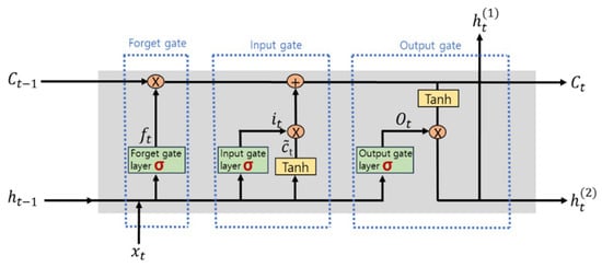
Figure 1.
Network structure of LSTM [26].
In this study, a total of 456 units were used across three LSTM layers: 256 units in the first layer, 128 units in the second, and 72 units in the third. The Adam optimizer was employed for model training.
The input variables for the LSTM model were constructed by incorporating not only the predicted PM2.5 values for the past 12 h, the forecast time, and the following 72 h, but also the predicted values of air quality and meteorological variables for the next 72 h.
The training period for the LSTM model spans approximately four years, from 1 January 2019 to 30 November 2022, while the evaluation period corresponds to the fourth phase of the Seasonal PM Management (1 December 2022–31 March 2023). The LSTM model is structured to utilize three days of chemical transport model forecast data as input to predict the same three-day forecast period (Figure 2).
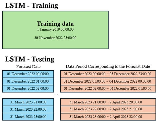
Figure 2.
Training and test datasets of LSTM.
2.4. SARIMAX
The AR (Auto Regressive) model constructs a predictive model based on the observed values of time series data, where the current value depends on past values. The MA (Moving Average) model, on the other hand, generates predictions based on past forecast errors, explaining the current observation as a linear combination of residual errors from previous time points. To handle non stationary data that cannot be effectively analyzed using AR and MA alone, differencing is introduced, leading to the development of the ARIMA model.
ARIMA models are categorized based on the presence of seasonality (Seasonal) and exogenous variables (Exogenous), as illustrated in Figure 3. The SARIMAX model, which is employed in this study, extends ARIMA by incorporating both seasonal and exogenous components, enhancing its predictive capability for complex time series data.
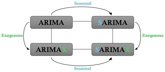
Figure 3.
Four models produced by seasonal and exogenous variables.
The SARIMAX model utilizes the predicted PM2.5 values for the past 12 h, the forecast time, and the following 72 h as input data.
For the SARIMAX model, training is conducted using historical data from the 15 days preceding the forecast time, which serves as the input dataset. The evaluation period is identical to that of the LSTM model. Like LSTM, SARIMAX receives three days of chemical transport model forecast data input to predict PM2.5 concentrations for the same period. The training and forecasting structures of LSTM and SARIMAX are illustrated in Figure 2 and Figure 4.
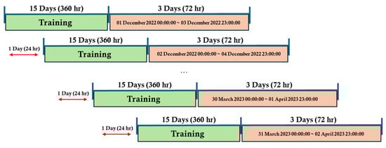
Figure 4.
Training and test datasets of SARIMAX.
The 72 h forecast results from the LSTM and SARIMAX models are divided into three periods: 1–24 h, 25–48 h, and 49–72 h, corresponding to D00 (today), D01 (tomorrow), and D02 (the day after tomorrow), respectively. The performance during each forecast period is analyzed and evaluated accordingly.
2.5. Model Evaluation Metrics
To evaluate the performance of the models, this study utilizes statistical metrics, including IOA (Index of Agreement), MBIAS (Mean Bias), RMSE (Root Mean Square Error), and r (correlation coefficient), along with forecasting indices such as ACC (Accuracy), POD (Probability of Detection), and FAR (False Alarm Rate).
The statistical metrics IOA, MBIAS, RMSE, and r can be expressed using Equations (1)–(4). In these equations, represents the observed pollutant concentration, while denotes the forecasted value produced by the model. The mean values of and are denoted as and , respectively, and refers to the total number of data points.
Figure 5 presents a matrix comparing observed and forecasted PM2.5 concentrations based on a threshold of 35 μg/m3. The concentration levels are further classified into four categories—Good, Moderate, Bad, and Very Bad—using thresholds of 15 μg/m3, 35 μg/m3, and 75 μg/m3. The results are analyzed based on these classifications.
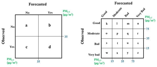
Figure 5.
Matrix of ACC, POD, FAR.
Using this matrix, the equations for ACC, POD, and FAR are formulated as Equations (5)–(7).
3. Results and Discussion
3.1. Hyper Parameter Optimization
Hyper parameters refer to tunable parameters within a model that must be manually configured by the user to construct an effective predictive system. In this study, the hyper parameters were adjusted separately for LSTM and SARIMAX to optimize model performance.
For LSTM, the primary hyper parameters modified were Epoch, Learning Rate, and Batch Size. The Epoch parameter was controlled using an early stopping mechanism, which terminated training when no further improvement in validation loss was observed, thereby preventing overfitting. The Learning Rate was dynamically adjusted through a Learning Rate reduction scheduler, allowing the model to fine tune its updates efficiently. The Batch Size was fixed at 64, ensuring consistency across all experiments.
For SARIMAX, the optimized hyper parameters included p, d, q, P, D, Q, and s. The auto_arima function (pm.auto_arima) was employed to explore various parameter combinations, selecting the optimal configuration based on the lowest AIC (Akaike Information Criterion) value and the shortest model training time. Additionally, SARIMAX hyper parameters were extracted for each specific evaluation date within the study period to ensure adaptive optimization.
The optimal hyper parameters for LSTM are presented in Table 2, while the SARIMAX hyper parameter results are not included in this paper.
Table 2.
Optimal hyper parameters for LSTM.
3.2. Model Evaluation
The forecast results for Seoul were evaluated through statistical analysis and time series analysis for D00 (today), D01 (tomorrow), and D02 (the day after tomorrow). The PM2.5 forecast results for Seoul are presented in Table 3 and Figure 6, Figure 7 and Figure 8.
Table 3.
Statistical forecast evaluation of CMAQ, LSTM, SARIMAX in Seoul.
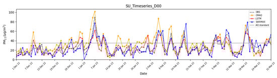
Figure 6.
Time series of PM2.5 concentrations for CMAQ, LSTM, and SARIMAX in Seoul during D00.
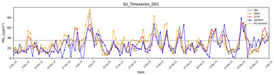
Figure 7.
Time series of PM2.5 concentrations for CMAQ, LSTM, and SARIMAX in Seoul during D01.
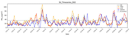
Figure 8.
Time series of PM2.5 concentrations for CMAQ, LSTM, and SARIMAX in Seoul during D02.
In D00, the SARIMAX model indicated superior predictive performance compared to both the LSTM and CMAQ models across all statistical evaluation metrics. In particular, SARIMAX corrected the overestimation of CMAQ forecast concentration, reducing the Mean Bias from 6.33 to −0.52, and achieved a correlation coefficient exceeding 0.85. The forecast skill score also improved, with the POD increasing by 19.43%, indicating SARIMAX’s enhanced ability to detect high PM2.5 concentrations in D00. Additionally, both the ACC and FAR improved. However, as the forecast period extended to D01 and D02, the performance of SARIMAX declined across all statistical evaluation metrics and forecast indices. This decline is attributed to the model’s reliance on short-term learning (using only the past 15 days of data), which enables strong short-term predictions (D00) but limits its capacity for long-term forecasting (D01-D02). Furthermore, statistical models like SARIMAX, when trained over an extended period, tend to capture the average trends of long-term data rather than diverse patterns such as high- and low-concentration episodes, suggesting that prolonged training may not necessarily enhance predictive performance. In addition, SARIMAX is based on short-term time series characteristics, which limits its ability to capture rapid fluctuations in future values.
The LSTM model demonstrated improved statistical evaluation metrics and forecast indices (except for POD) compared to the CMAQ results in D00. However, its performance declined across all statistical metrics compared to SARIMAX. Nevertheless, as the forecast lead time increased from D00 to D02, LSTM outperformed both CMAQ and SARIMAX in predictive performance.
These results suggest that LSTM excels in learning various data patterns such as high- and low-concentration episodes due to its ability to train on four years of historical data, unlike SARIMAX. Specifically, its ability to preserve long-term patterns enhances its effectiveness in making extended-range forecasts. This characteristic represents the fundamental distinction between deep learning models such as LSTM and statistical models like SARIMAX.
Examining the temporal patterns shows that SARIMAX closely replicated high and low concentrations in D00, aligning well with the observed concentrations. However, on 2 January 2023, it tended to underestimate concentrations compared to measurements, exhibiting negative bias. This tendency became more frequent as the forecast progressed to D01 and D02, suggesting that the derived multi-variable equation approach contributes to long-term forecasting issues. Consequently, as the prediction advanced to D01 and D02, SARIMAX struggled to accurately capture the time series patterns of the observed concentrations. As such, SARIMAX exhibited tendencies to overestimate and underestimate under high- and low-concentration conditions, respectively. This can be interpreted as a limitation of its linear-based structure, which fails to capture nonlinear and abrupt changes in the data.
The LSTM model largely exhibits temporal characteristics similar to those of chemical transport models such as CMAQ and demonstrates patterns comparable to the observed concentrations. However, while the chemical transport model tends to overestimate concentrations in most cases, the LSTM model more closely aligns with the observed concentration levels. Furthermore, compared to the SARIMAX model, the LSTM model exhibits a similar trend to the observed concentrations even in long-term forecasts. Because deep learning training incorporates nonlinearity, LSTM, unlike SARIMAX, did not produce negative concentration predictions on 2 January 2023. In contrast, the LSTM model tended to follow the forecast patterns of the numerical model under certain high-concentration conditions. This is likely because the primary input data for the LSTM were based on the outputs of the numerical model, leading the LSTM to learn the nonlinear forecast patterns that occur during high-concentration events.
3.3. High PM2.5 Concentration Analysis
To analyze periods of high PM2.5 concentration, episodes in which the daily and hourly PM2.5 concentration in Seoul exceeded 35 μg/m3 were selected. The model evaluation results for these high-concentration periods are presented in Table 4 and Table 5.
Table 4.
Statistical forecast evaluation of CMAQ, LSTM, and SARIMAX in Seoul during periods of high PM2.5 concentration (daily analysis).
Table 5.
Statistical forecast evaluation of CMAQ, LSTM, and SARIMAX in Seoul during high-PM2.5 concentration periods (hourly analysis).
As the forecast progressed from D00 to D02, the LSTM model exhibited a decline in forecast indices and statistical metrics compared to the overall period (December 2022–March 2023), except for POD and FAR. However, despite the increase in forecast lead time, the forecast consistency did not deteriorate significantly; instead, it remained stable and even improved in some cases. These findings suggest that the LSTM model has strong applicability for air quality forecasting, particularly for high-PM2.5 concentration events.
On the other hand, SARIMAX demonstrated superior predictive performance in D00 compared to the other two models (CMAQ and LSTM), with particularly high POD values. However, a sharp decline in model performance occurred from D00 onward. These results indicate that while SARIMAX outperforms LSTM in short-term (D00) PM2.5 forecasting under high-concentration conditions, its performance deteriorates in long-term forecasts (D01 to D02).
The results of the hourly high PM2.5 concentration analysis exhibited comparable statistical results and trends to the daily average analysis. As the forecast lead time increased, the LSTM model showed an improved predictive performance, while SARIMAX demonstrated superior accuracy at the shortest lead time (D00). However, the statistical performance of the hourly analysis was not in agreement with the observations data compared with daily-scale analysis. This discrepancy may be attributed to the fact that daily data tend to smooth out high-frequency fluctuations in PM2.5 concentrations, thereby compensating for the model’s limited ability to capture abrupt, short-term variations in PM2.5 concentration (Table 5).
4. Conclusions
This study conducted a performance evaluation of LSTM and SARIMAX in terms of PM2.5 forecasting in Seoul, South Korea, focusing on forecast lead times (D00–D02).
For short-term forecasting (D00), SARIMAX outperformed LSTM in all statistical evaluation metrics, particularly in detecting high PM2.5 concentrations, with a 19.43% higher Probability of Detection (POD). For extended forecasting (D01–D02), SARIMAX’s performance deteriorated significantly, while LSTM maintained relatively better accuracy over D01 and D02.
Under high-concentration conditions, LSTM exhibited better predictive capabilities in capturing PM2.5 peaks, while SARIMAX showed greater performance degradation over time. Under low-concentration conditions, LSTM struggled to capture short-term variations, indicating a tendency to focus on overall trends rather than local fluctuations.
In summary, statistical models offer advantages in short-term forecasting and require less training data compared to deep learning models. Conversely, deep learning models exhibit significant strengths in long-term forecasting and maintaining a stable predictive performance. Overall, both models demonstrated superior forecasting performance compared to chemical transport models. These findings emphasize the necessity of an integrated air quality forecasting system that leverages the strengths of numerical, statistical, and machine learning approaches.
This study has several limitations that should be acknowledged, along with directions for future research. The predictive models analyzed in this work inherently include uncertainties arising from both the input data and the modeling frameworks themselves. Among these, the most significant source of error is likely the input model. Specifically, the CMAQ model, which serves as the input, is subject to uncertainties in meteorological variables, emission inventories, and chemical mechanisms. These errors are not only inherent, but can also accumulate or be amplified throughout the modeling process, thereby influencing the overall performance. Consequently, the accuracy and reliability of the forecasting model used, such as statistic and AI models, are highly dependent on the quality and precision of the input model.
In addition, the statistical and artificial intelligence models used in this study also contain intrinsic limitations. The SARIMAX model constructs statistical functions based on recent forecasting data; however, it may fail to capture abrupt fluctuations in pollutant concentrations. Moreover, it generates negative concentration values and exhibits reduced accuracy when applied to long-term predictions of identical functions. Similarly, while LSTM models demonstrate strengths in handling sequential data, they are constrained by their limited long-term memory capacity. This suggests the need to adopt more advanced deep learning architectures that can better handle temporal dependencies and nonlinear patterns in future work.
Future studies are encouraged to improve input data accuracy, possibly by integrating higher-resolution meteorological and emissions data, and to explore alternative or hybrid AI approaches that can better accommodate the complexities of air quality dynamics.
Author Contributions
Conceptualization, D.-R.C.; methodology, J.-Y.L. and J.-G.K.; validation, D.-R.C. and J.-B.L.; formal analysis, C.-Y.L. and S.-H.H.; investigation, C.-Y.L. and S.-H.H.; data curation, D.-R.C. and J.-Y.L.; writing—original draft preparation, C.-Y.L.; writing—review and editing, C.-Y.L. and J.-B.L.; supervision, D.-R.C. and J.-G.K.; funding acquisition, D.-R.C. All authors have read and agreed to the published version of the manuscript.
Funding
This research received no external funding.
Institutional Review Board Statement
Not applicable.
Informed Consent Statement
Not applicable.
Data Availability Statement
The data presented in this study are available on request from the corresponding author.
Conflicts of Interest
The authors declare no conflicts of interest.
References
- Seinfeld, J.-H.; Pandis, S.-N. Atmospheric Chemistry and Physics: From Air Pollution to Climate Change, 3rd ed.; John Wiley & Sons Inc: Hoboken, NJ, USA, 2016. [Google Scholar]
- Kampa, M.; Castanas, E. Human health effects of air pollution. Environ. Pollut. 2007, 151, 362–367. [Google Scholar] [CrossRef] [PubMed]
- Nam, K.-P.; Lee, D.-G.; Jang, L.-S. Analysis of PM2.5 concentration and contribution characteristics in South Korea according to seasonal weather patterns in East Asia: Focusing on the intensive measurement periods in 2015. J. Environ. Impact Assess. 2019, 28, 183–200. [Google Scholar] [CrossRef]
- Choi, J.-K.; Choi, I.-S.; Cho, K.-K.; Lee, S.-H. Harmfulness of particulate matter in disease progression. J. Life Sci. 2020, 30, 191–201. [Google Scholar] [CrossRef]
- MSIP (Ministry of Science, ICT and Future Planning). R&D Strategy Against Particulate Matter Pollution. 2016. Available online: https://www.msit.go.kr/eng/index.do (accessed on 20 April 2025).
- Chang, L.-S.; Cho, A.; Park, H.-J.; Nam, K.-P.; Kim, D.-K.; Hong, J.-H.; Song, C.-K. Human-model hybrid Korean air quality forecasting system. J. Air Waste Manag. Assoc. 2016, 66, 896–911. [Google Scholar] [CrossRef] [PubMed]
- Koo, Y.-S.; Kwon, H.-Y.; Bae, H.-S.; Yun, H.-Y.; Choi, D.-R.; Yu, S.-H.; Wang, K.-H.; Koo, J.-S. A development of PM2.5 forecasting system in South Korea using chemical transport modeling and machine learning. Asia-Pac. J. Atmos. Sci. 2023, 59, 577–595. [Google Scholar] [CrossRef]
- Choi, C.-C.; Lim, Y.-J.; Lee, J.-B.; Nam, K.-P.; Lee, H.-S.; Lee, Y.-H.; Myoung, J.-S.; Kim, T.-H.; Jang, L.-S.; Kim, J.-S.; et al. Evaluation of the simulated PM2.5 concentrations using air quality forecasting system according to emission inventories—Focused on China and South Korea. J. Korean Soc. Atmos. Environ. 2018, 34, 306–320. [Google Scholar] [CrossRef]
- Lin, C.-J.; Ho, T.-C.; Chu, H.-W.; Yang, H.; Chandru, S.; Krishnarajanagar, N.; Chiou, P.; Hopper, J.-R. Sensitivity analysis of ground-level ozone concentration to emission changes in two urban regions of southeast Texas. J. Environ. Manag. 2005, 75, 315–323. [Google Scholar] [CrossRef]
- Ho, C.-H.; Park, I.-G.; Oh, H.-R.; Gim, H.-J.; Hur, S.-K.; Kim, J.-O.; Choi, D.-R. Development of a PM2.5 prediction model using a recurrent neural network algorithm for the Seoul metropolitan area. Atmos. Environ. 2021, 245, 118021. [Google Scholar] [CrossRef]
- Chu, Y.; Liu, Y.; Li, X.; Liu, Z.; Liu, H.; Lu, Y.; Mao, Z.; Chen, X.; Li, N.; Ren, M.; et al. A review on predicting ground PM2.5 concentration using satellite aerosol optical depth. Atmosphere 2016, 7, 129. [Google Scholar] [CrossRef]
- Chen, J.; Hoogh, K.; Gulliver, J.; Hoffmann, B.; Hertel, O.; Ketzel, M.; Bauwelinck, M.; Donkelaar, A.; Hvidtfeldt, U.-A.; Katsouyanni, K.; et al. A comparison of linear regression, regularization, and machine learning algorithms to develop Europe-wide spatial models of fine particles and nitrogen dioxide. Atmosphere 2019, 130, 104934. [Google Scholar] [CrossRef]
- He, Z.-F.; Guo, Q.-C. Comparative Analysis of Multiple Deep Learning Models for Forecasting Monthly Ambient PM2.5 Concentrations: A Case Study in Dezhou City, China. Atmosphere 2024, 15, 1432. [Google Scholar] [CrossRef]
- He, Z.-F.; Guo, Q.-C.; Wang, Z.-S.; Li, X.-Z. Prediction of Monthly PM2.5 Concentration in Liaocheng in China Employing Artificial Neural Network. Atmosphere 2022, 13, 1221. [Google Scholar] [CrossRef]
- Guo, Q.-C.; He, Z.-F.; Wang, Z.-S. Prediction of Hourly PM2.5 and PM10 Concentrations in Chongqing City in China Based on Artificial Neural Network. Aerosol Air Qual. Res. 2023, 23, 220448. [Google Scholar] [CrossRef]
- Lee, J.-Y.; Lee, C.-Y.; Jung, M.-W.; Ahn, J.-Y.; Choi, D.-R.; Yun, H.-Y. XAI Analysis of DNN Using PM2.5 Component Input Data and Improvement of PM2.5 Prediction Performance. J. Korean Soc. Atmos. Environ. 2023, 39, 411–426. [Google Scholar] [CrossRef]
- Hochreiter, S.; Schmidhuber, J. Long short-term memory. Neural Comput. 1997, 9, 1735–1780. [Google Scholar] [CrossRef]
- Gers, F.-A.; Schmidhuber, J.; Cummins, F. Learning to forget: Continual prediction with LSTM. Neural Comput. 2000, 12, 2451–2471. [Google Scholar] [CrossRef] [PubMed]
- Dutta, J.; Roy, S. IndoorSense: Context-based indoor pollutant prediction using SARIMAX model. Multimed. Tools Appl. 2021, 80, 19989–20018. [Google Scholar] [CrossRef]
- William, W.-S. Time Series Analysis: Univariate and Multivariate Methods; Wesley Publishing: Philadelphia, PA, USA, 2006. [Google Scholar]
- Ni, X.-Y.; Huang, H.; Du, W.-P. Relevance analysis and short-term prediction of PM2.5 concentrations in Beijing based on multi-source data. Atmos. Environ. 2017, 150, 146–161. [Google Scholar] [CrossRef]
- Knaak, J.; de Paula Pinto, W. Application of SARIMAX model to model and forecast the concentration of inhalable particulate matter, in Espírito Santo, Brazil. Ciência E Nat. 2022, 44, 9. [Google Scholar] [CrossRef]
- Kang, J.-G.; Lee, J.-Y.; Lee, J.-B.; Lim, J.-H.; Yun, H.-Y.; Choi, D.-R. High-resolution daily PM2.5 exposure concentrations in South Korea using CMAQ data assimilation with surface measurements and MAIAC AOD (2015–2021). Atmosphere 2024, 15, 1152. [Google Scholar] [CrossRef]
- Choi, D.-R.; Yun, H.-Y.; Koo, Y.-S. A development of air quality forecasting system with data assimilation using surface measurements in East Asia. J. Korean Soc. Atmos. Environ. 2019, 35, 60–85. [Google Scholar] [CrossRef]
- Zhao, Z.; Chen, W.; Wu, X.; Chen, P.C.; Liu, J. LSTM network: A deep learning approach for short-term traffic forecast. IET Intell. Transp. Syst. 2017, 11, 68–75. [Google Scholar] [CrossRef]
- Xie, M.; Shi, Z.; Yue, X.; Ding, M.; Qiu, Y.; Jia, Y.; Li, B.; Li, N. Fault Diagnosis and Prediction System for Metal Wire Feeding Additive Manufacturing. Sensors 2024, 24, 4277. [Google Scholar] [CrossRef] [PubMed]
Disclaimer/Publisher’s Note: The statements, opinions and data contained in all publications are solely those of the individual author(s) and contributor(s) and not of MDPI and/or the editor(s). MDPI and/or the editor(s) disclaim responsibility for any injury to people or property resulting from any ideas, methods, instructions or products referred to in the content. |
© 2025 by the authors. Licensee MDPI, Basel, Switzerland. This article is an open access article distributed under the terms and conditions of the Creative Commons Attribution (CC BY) license (https://creativecommons.org/licenses/by/4.0/).