Unveiling Cloud Microphysics of Marine Cold Air Outbreaks Through A-Train’s Active Instrumentation

Abstract

Marine Cold Air Outbreaks (MCAOs) are critical drivers of high-latitude climates because they regulate the exchange of heat, moisture, and momentum between cold continental or polar air masses and relatively warmer ocean surfaces. In this study, we combined CloudSat–CALIPSO observations (2007–2017) with ERA5 reanalysis data to investigate the microphysical properties and vertical structure of snowfall during MCAOs. By classifying events using a low-level instability parameter, we provide a detailed comparison of the vertical and spatial characteristics of different snowfall regimes, focusing on key cloud properties such as the effective radius, particle concentration, and ice water content. Our analysis identified two distinct snowfall regimes: shallow stratocumulus-dominated snowfall, prevalent during typical MCAOs and characterized by cloud top heights below 3 km and a comparatively lower ice water content (IWC), and deeper snowfall occurring during non-CAO conditions. We demonstrate that, despite their lower instantaneous snowfall rates, CAO-related snowfall events cumulatively contribute significantly to the total ice mass production in the subpolar North Atlantic. Additionally, CAO events are characterized by a greater number of ice particles near the surface, which are also smaller ($r_{\mathrm{eff}}$ of 59 μm versus 62 μm) than those associated with non-CAO events. These microphysical differences impact cloud optical properties, influencing the surface radiative balance.

1. Introduction

Cold Air Outbreaks (CAOs) are a fundamental component of the Earth’s energy balance, playing a crucial role in regulating heat exchange between the atmosphere, ocean, and cryosphere. These events, characterized by the advection of cold, dry air from polar or continental regions over relatively warmer ocean waters, induce strong turbulent heat fluxes that significantly impact both local and global atmospheric circulations [1]. The interaction between cold air and warm ocean surfaces results in the destabilization of the lower troposphere, leading to enhanced cloud formation, precipitation, and the modification of the surface radiative budget [2]. These processes contribute to the redistribution of heat and moisture across latitudes, influencing weather patterns far beyond the outbreak regions.

In the North Atlantic region, CAOs are particularly significant due to their impact on the regional climate, weather variability, and socio-economic activities. The advection of Arctic air masses over the Nordic and Barents Seas triggers intense cloud formation and precipitation, often leading to hazardous weather conditions such as snowfall and strong winds [3]. These events play a key role in ocean–atmosphere interactions, driving deep convection and influencing thermohaline circulation, which is vital for the stability of the Atlantic Meridional Overturning Circulation (AMOC) [4]. Furthermore, CAOs are frequently associated with polar lows, small but intense maritime cyclones that pose significant risks to marine and coastal operations [4]. Given the increasing variability of Arctic climate conditions, understanding CAOs is critical for improving weather predictions and climate models that affect millions of people in northern Europe and beyond.

A critical aspect of CAOs is their vertical cloud structure, which drives their radiative properties and precipitation effects. Unlike synoptic-scale snowstorms, often driven by large baroclinic systems with deep cloud layers, CAO-induced snowfall is typically associated with shallow convective cloud regimes [1]. Observations from satellite-based remote sensing indicate that snowfall within CAOs is frequently generated by stratocumulus clouds with cloud top heights below 3 km, although stronger events may exhibit deeper convective structures [1]. Snowfall rates in CAOs are generally light (<0.1 mm/h liquid water equivalent) compared to the more intense precipitation associated with polar lows and extratropical cyclones [1]. The cloud morphology in CAOs resembles open-cellular convection, transitioning from cloud streets to shallow stratocumulus, differing significantly from the deep, organized cloud layers found in extratropical cyclones and polar lows [4].

Moreover, CAO clouds are dominated by supercooled liquid water, unlike the deep mixed-phase clouds typical of frontal cyclones [2]. The presence of strong boundary layer inversions in CAOs prevents deep convective development, whereas frontal snow systems are dynamically forced by large-scale baroclinic lifting [1]. In addition, CAO-induced snowfall is influenced by the length of the air mass fetch over the ocean, with longer fetches promoting deeper convection and higher snowfall rates [1].

Recent observational and modeling studies have highlighted significant uncertainties in our understanding of cloud microphysical processes associated with marine CAOs. Despite the recognized importance of these events for high-latitude climates, numerical weather and climate models continue to struggle in accurately simulating the evolution of cloud phases and precipitation within CAOs. Key modeling challenges include the premature glaciation of mixed-phase clouds, the underestimation of supercooled liquid water layers, and uncertainties in representing secondary ice production (SIP), the riming efficiency, and particle growth mechanisms [5,6]. Observationally, these uncertainties are exacerbated by the remote locations and harsh conditions characteristic of CAO regions, which significantly limit the availability and quality of in situ microphysical measurements [7,8]. Satellite remote sensing platforms provide broad coverage but face their own challenges, including biases related to mixed-phase cloud retrievals, surface clutter near the cloud base, and limitations in distinguishing cloud phases within vertically heterogeneous cloud structures [1,9].

This study directly addressed several of these observational and modeling gaps by utilizing combined active remote sensing observations from CloudSat and CALIPSO satellites. The unique synergy of radar and lidar sensors aboard these platforms provides the comprehensive vertical profiling of cloud and snowfall structures, capturing both ice precipitation and supercooled liquid cloud layers across extensive marine regions. Specifically, our analysis characterized two distinct snowfall regimes associated with CAOs: shallow stratocumulus-dominated systems and deeper cumuliform clouds observed under intense CAO conditions. Such vertical and horizontal differentiation in snowfall characteristics and cloud top structures helps elucidate how microphysical processes such as riming, depositional growth, and secondary ice formation vary across different outbreak intensities and atmospheric stability conditions, addressing previously identified gaps [10,11].

Additionally, our findings contribute novel observational benchmarks for model validation, particularly in the representation of cloud top liquid layers and vertical phase partitioning, critical aspects that models often misrepresent. By systematically classifying and comparing snowfall events under CAO and non-CAO conditions using satellite-derived vertical reflectivity profiles and collocated reanalysis stability metrics, this work advanced our understanding of the cloud microphysical processes governing precipitation during marine CAOs. Ultimately, these insights will help constrain microphysical parameterizations in models, enhancing predictive capabilities for weather and climate systems affected by CAOs at high latitudes [12,13].

In this study, we integrated reanalysis data from the European Centre for Medium-Range Weather Forecasts (ECMWF) with CloudSat–CALIPSO cloud retrievals to investigate the vertical structure and spatial distribution of snowfall during Marine Cold Air Outbreaks (MCAOs) over the North Atlantic Ocean. By focusing exclusively on snowfall and excluding mixed-phase and liquid precipitation, we highlighted the influence of MCAOs on the widespread shallow snowfall observed using CloudSat. Snow microphysics estimates and vertical reflectivity profiles from CloudSat–CALIPSO (2007–2017) were analyzed alongside an ERA5-derived MCAO flag to examine differences between snowfall events associated with MCAOs and those occurring under “non-CAO” conditions. Section 2 outlines the data and methodology used to classify events into MCAO and non-CAO categories. Section 3 presents the key findings of the study, while Section 4 offers concluding remarks.

2. Data and Methods

CloudSat, a key component of NASA’s A-Train satellite constellation [14], featured a W-band cloud profiling radar (CPR) that operated at 94 GHz. This radar was uniquely designed to provide high-resolution vertical profiles of clouds and precipitation, offering high sensitivity to detect a wide range of hydrometeors, from light snow and drizzle to moderate rain. The CPR measured the backscattered energy from atmospheric particles, enabling detailed observations of the vertical structure of clouds and precipitation systems. From its launch in April 2006 until the end of its operational life in December 2023, CloudSat significantly enhanced our understanding of cloud microphysics, cloud–aerosol interactions, and precipitation processes. It also demonstrated the feasibility and scientific value of active remote sensing from space, producing a wealth of data widely used in atmospheric and climate research.

In particular, CloudSat revolutionized global snowfall detection, offering unprecedented insights into snowfall processes up to an 82° latitude [15,16,17,18]. Its high sensitivity allowed for the identification of unique snowfall regimes, such as cumuliform snowfall [19], which were previously challenging to observe on a near-global scale. A comprehensive assessment of the CloudSat CPR’s capabilities in monitoring snowfall across different temporal and spatial scales was provided by Kulie et al. [20]. Moreover, a recent validation study by Mroz et al. [21] comparing snowfall rate estimates from the CloudSat CPR and GPM products found that CloudSat retrievals exhibited significantly higher agreement with ground-based radar measurements than other satellite-based snowfall retrieval algorithms. These advancements underscore the critical role of CloudSat in improving global snowfall climatology and refining snowfall parameterizations in numerical weather and climate models.

The CALIPSO mission, launched in April 2006, was designed to provide insights into the vertical structure and distribution of aerosols and clouds, addressing critical uncertainties in their roles within the Earth’s climate system [22]. CALIPSO operates as part of the A-Train satellite constellation, combining its unique lidar instrument, Cloud–Aerosol Lidar with Orthogonal Polarization (CALIOP), with passive sensors such as a Wide-Field Camera (WFC) and an Imaging Infrared Radiometer (IIR). CALIOP is a polarization-sensitive lidar capable of capturing high-resolution vertical profiles of clouds and aerosols, distinguishing between their types and layers. This capability has been instrumental in characterizing optically thin clouds, such as cirrus, and aerosol layers overlying clouds, both of which significantly influence the Earth’s radiative budget. The synergy of active and passive sensors on board CALIPSO, along with collocated observations from other A-Train satellites, allows for comprehensive analyses of cloud and aerosol interactions, their radiative effects, and their spatial and temporal variability. By addressing gaps in previous observational datasets, CALIPSO has significantly improved the accuracy of climate models and weather prediction systems, providing a robust foundation for understanding aerosol–cloud–climate interactions.

In this study, we utilized the CloudSat–CALIPSO DARDAR (radar–lidar) product [23] to analyze the vertical structure of snowfall during Marine Cold Air Outbreaks. The DARDAR product employs a variational retrieval scheme that combines measurements from CloudSat’s cloud profiling radar (CPR) and CALIPSO’s CALIOP, along with auxiliary infrared radiometer data, to derive ice cloud microphysical properties with a high vertical resolution. This method enables the seamless retrieval of the ice water content, visible extinction coefficient, and effective radius across regions where either radar, lidar, or both instruments provide valid measurements. In our analysis, we used the version of the DARDAR algorithm that incorporates the Brown and Francis [24] mass–size relationship for ice particles, ensuring consistency in ice microphysical property estimation. The radar reflectivity data were obtained from the 2B-GEOPROF product [25]. A list of the data products used in this article is given in

Table 1. Summary of satellite and reanalysis datasets used.

Dataset	Period	Horizontal Resolution	Vertical Resolution
CloudSat CPR	2007–2017	1.4 km	240 m
CALIPSO Lidar	2007–2017	333 m	30–60 m
DARDAR Product	2007–2017	1.4 km	60 m
ERA5 Reanalysis	2007–2017	0.25°	Multiple pressure levels

. We acknowledge that CloudSat’s limited temporal sampling frequency, with an approximate 16-day revisit cycle, may have introduced sampling biases, particularly for transient snowfall events, potentially affecting the statistical representativeness of our analysis. However, a detailed uncertainty analysis conducted by Scarsi et al. [26] demonstrated that CloudSat’s retrievals reliably reproduce annual snowfall patterns despite these sampling constraints. Consequently, our extensive dataset covering 11 years provided sufficiently robust statistics for the purposes of this study.

A distinctive feature of the DARDAR algorithm is the rigorous handling of observational uncertainties and the thoughtful selection of state variables along with appropriate a priori assumptions. This design ensures smooth and continuous retrievals across regions where both radar and lidar data are available and seamless transitions into regions where only one instrument detects the cloud [27]. Specifically, when lidar measurements become unavailable due to severe attenuation (e.g., in dense ice clouds), the retrieval naturally shifts toward using empirical relationships between the radar reflectivity and atmospheric temperature. Conversely, when radar observations are not available, as in optically thin cirrus clouds, the algorithm still provides robust retrievals by integrating lidar signals with radiometric measurements.

In addition to the ice water content estimates, we computed the total ice mass observed during our analysis period, following the methodology described below:

• Ice Water Path Calculation: We first used the retrieved ice water content (IWC, in kg/${\mathrm{m}}^3$) across the vertical radar profile to obtain the ice water path (IWP, in kg/${\mathrm{m}}^2$) for each CloudSat radar footprint. This represented the total ice mass per unit area in the atmospheric column.
• Total Ice Mass Per Profile: To obtain the total ice mass per radar footprint, we multiplied the IWP by the footprint area (approx. 1.4 km × 1.8 km $\times \pi$).
• Spatial Aggregation: The total ice mass from all footprints was then summed within each 2 × 2 degrees latitude–longitude grid cell to provide a spatially resolved estimate.
• Normalization by the Grid Area: Since grid cell areas varied with the latitude, we normalized the total ice mass in each grid cell by the corresponding geometrical area of the grid cell to allow for a fair comparison across regions.

To distinguish between CAO and non-CAO events, we adopted the methodology outlined by [1]. Specifically, we calculated the M parameter, defined as the difference between the sea surface potential temperature and the potential temperature at 850 hPa, using data from the ERA5 reanalysis provided by the European Centre for Medium-Range Weather Forecasts (ECMWF), which are archived in the CloudSat ECMWF-AUX files. The M parameter was indicative of the lower-tropospheric instability. This approach allowed for a systematic identification of CAO and non-CAO conditions.

In this study, we refined the classification criteria to improve the separation between CAO and non-CAO events and minimize the impact of borderline cases that could skew the statistics. In particular, we excluded all events with $\left|M\right|<5$ K from classification, labeling them as unclassified. Events with $M>5$ K were classified as CAOs, indicating strong lower-tropospheric instability and the presence of CAOs. Conversely, events with $M<-5$ K were categorized as non-CAOs, reflecting stable conditions typical of synoptic-scale systems. This convention ensured a clearer distinction between the two regimes, enhancing the robustness of the statistical analysis. We acknowledge that the choice of the $\left|M\right|>5$ K threshold for classification was somewhat arbitrary, as it was primarily determined based on the visual inspection of multiple case studies. This value was selected to minimize ambiguity in event classification, reducing the number of borderline cases that were difficult to categorize through visible satellite imagery alone. While this method enhanced clarity in distinguishing CAO from non-CAO events, further sensitivity tests could quantify the impact of this threshold on the classification robustness. While our classification clearly distinguished strong CAO events (highly unstable, $M>5$ K), the “non-CAO” label (stable conditions, $M<-5$ K) broadly represented events associated predominantly with synoptic-scale forcing, such as frontal systems and extratropical cyclones. Although we recognize that not every “non-CAO” event may correspond strictly to frontal snowfall, the majority of snowfalls occurring under these stable lower-tropospheric conditions typically result from dynamic large-scale processes rather than convective instability. Thus, interpreting the “non-CAO” category as representative of frontal snowfall regimes was broadly justified and helped in understanding the contrasting microphysical characteristics relative to those of the convectively driven CAO events.

The Known Limitations of the DARDAR Product

DARDAR-CLOUD retrievals provide vertical profiles of ice microphysical properties based on radar–lidar synergy from CloudSat and CALIPSO observations. However, the product has known limitations in situations where mixed-phase clouds and supercooled liquid layers occur, such as North Atlantic MCAOs. In these regions, supercooled liquid layers frequently exist at cloud tops, potentially attenuating the CALIPSO lidar signal due to strong optical extinction. Once the lidar signal is extinguished, the retrieval becomes radar-only, relying on climatological and empirical relationships between the radar reflectivity and temperature to constrain ice properties. This limitation implies that DARDAR-CLOUD profiles may not fully represent the vertical distribution of ice and snow properties when supercooled liquid water layers are present or have been present upstream along the lidar beam path [23,28,29].

Previous studies have documented these situations, noting that polar low systems and CAOs are often dominated by the ice phase but exhibit significant occurrences of supercooled liquid water layers, particularly near cloud tops or in convective updrafts [4]. The DARDAR-MASK product explicitly identifies these mixed-phase and supercooled liquid layers, but retrieval algorithms designed specifically for mixed-phase conditions are not included within the current DARDAR-CLOUD product [28].

In situations classified as mixed-phase by DARDAR-MASK, the current DARDAR-CLOUD retrieval procedure excludes the lidar measurements from regions identified as containing liquid droplets to avoid the contamination of the ice retrieval with signals from liquid water. Thus, retrievals in mixed-phase regions revert effectively to a radar-only algorithm, which implicitly assumes that the radar reflectivity is predominantly from ice particles. This approach means that supercooled liquid layers are not explicitly represented in the ice retrievals, potentially resulting in incomplete or biased ice cloud microphysical profiles in these conditions [28,29].

Additionally, the effects of riming, a common microphysical process in marine CAOs, are not explicitly accounted for in the DARDAR-CLOUD retrieval. Rimed particles typically possess higher densities and different fall speeds compared to unrimed ice crystals. The retrieval assumes generic ice particle properties derived from empirical relationships and does not currently incorporate adjustments to account specifically for riming effects [29].

As a consequence, the microphysical features characteristic of CAOs, such as an enhanced ice water content and altered effective radii due to riming and mixed-phase processes, may not be captured accurately by DARDAR-CLOUD. While the explicit frequency and impact of supercooled liquid layers and mixed-phase conditions in North Atlantic CAOs determined using DARDAR-MASK have not been detailed extensively in the literature, the overall methodology suggests that microphysical retrievals from DARDAR-CLOUD in these environments should be interpreted cautiously. A detailed statistical analysis using DARDAR-MASK data to quantify the frequency of mixed-phase occurrences in marine CAOs would further clarify these potential retrieval biases. However, in our analysis, we did not filter out profiles containing liquid clouds, as these profiles are an integral and representative component of Cold Air Outbreaks. We therefore acknowledge and accept that the derived ice cloud and snowfall properties may include biases associated with these mixed-phase conditions.

3. Results

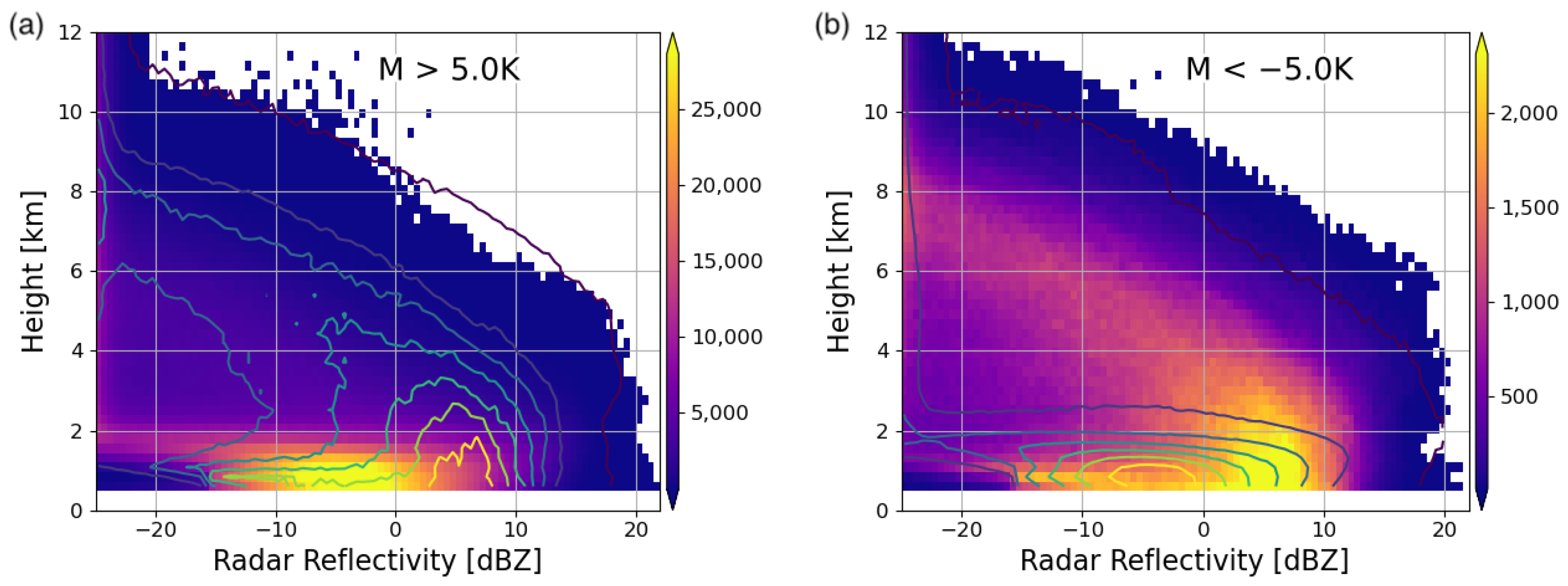
Figure 1 shows the Contour Frequency Altitude Diagram (CFAD) of the radar reflectivity for CAO and non-CAO events. The left panel highlights the characteristic shallow vertical structure of CAO phenomena: the detectable radar echoes rarely extended beyond 2 km ASL, underscoring the dominance of low-level clouds during CAOs. These observations align with prior studies indicating that CAO snowfall is primarily generated by shallow stratocumulus clouds with cloud top heights that are typically below 3 km [1]. The relatively lower reflectivity near the surface in the CAO events suggests a lower concentration of larger precipitation particles or a reduced overall precipitation rate. This could be attributed to the limited development of convective processes due to strong boundary layer inversions which suppressed vertical mixing and deeper cloud growth.

In contrast, the right panel, which represents non-CAO events, displays a markedly different vertical profile. Radar echoes extended much higher, often reaching altitudes above 8 km, indicative of deeper cloud systems such as nimbostratus or mixed-phase frontal clouds associated with extratropical cyclones. These systems exhibited higher radar reflectivity values near the surface, thus implying more intense precipitation and a greater presence of larger hydrometeors. The deeper vertical structure and higher reflectivity highlight the dynamic forcing mechanisms typical of non-CAO events, such as baroclinic instability and large-scale lifting, which promote significant cloud and precipitation development.

3.1. Ice Water Content

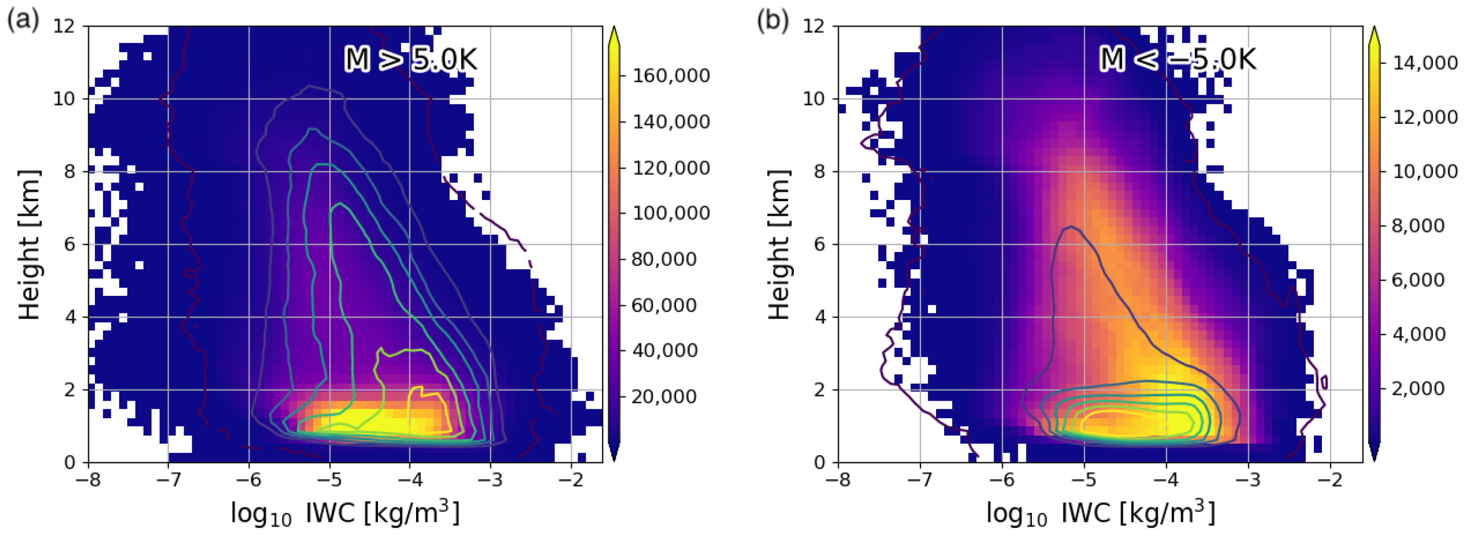
The comparison of IWC distributions between CAOs and other snowfall events revealed significant differences in both the vertical extent and concentration of ice masses (see Figure 2). Near the surface, non-CAO events showed a broader spread of ${log}_{10}$ IWC values, with the peak frequency exceeding ${10}^{-4}$ kg ${\mathrm{m}}^{-3}$. In CAO cases, the observed range of IWC values was narrower, and the peak frequency of the probability density function (PDF) shifted toward lower values, typically being between ${10}^{-5}$ and ${10}^{-4}$ kg ${\mathrm{m}}^{-3}$.

At higher altitudes, non-CAO events displayed a taller and broader distribution of the IWC, indicative of deeper cloud structures with more persistent ice production higher up. The presence of a significant ice mass above 3 km in these events suggests stronger synoptic or mesoscale forcing, supporting sustained cloud growth. In contrast, CAOs exhibited a shallower vertical IWC distribution, with a tighter spread at higher altitudes and a less pronounced ice-producing layer higher up.

3.2. Effective Radius

The vertical distribution of the retrieved effective radius ( $r_{\mathrm{eff}}$) for CAOs and non-CAO snowfall events, shown in Figure 3, highlights the distinct microphysical characteristics of these two regimes. Differences emerged in the spread and peak locations of $r_{\mathrm{eff}}$. For CAO events (Figure 3a), the effective radius distribution was narrower, with the highest frequencies of occurrence tightly clustered between 55 μm and 75 μm at altitudes below 2 km. Above this level, the frequency of occurrence decreased sharply. The narrower range of $r_{\mathrm{eff}}$ values resulted from limited vertical cloud development and constrained ice production due to strong boundary layer inversion [12].

In contrast, the non-CAO snowfall events (Figure 3b) exhibited a broader vertical distribution of $r_{\mathrm{eff}}$, with a notable high-frequency region spanning a wider range of effective radii between 60 μm and 90 μm. The extended distribution at higher altitudes suggests that ice growth processes were more sustained higher up, possibly due to higher supersaturation. Additionally, the contour overlays indicate that, relative to CAO events, non-CAO snowfall maintained a higher probability across a broader range of effective radius values at low altitudes, reinforcing the idea of a more diverse ice particle population.

These differences suggest that CAOs are characterized by a more constrained microphysical regime, where ice particle growth is limited in both the vertical extent and maximum size. Meanwhile, the broader $r_{\mathrm{eff}}$ distributions in non-CAO events imply more efficient ice growth, potentially influenced by a more favorable environment.

3.3. Spatial Characteristics of Cold Air Outbreaks

In order to analyze the spatial occurrence patterns of CAO and non-CAO events, we analyzed CloudSat radar measurements collected from 2007 to 2017 and classified them using the low-level instability parameter M, as described in Section 2. Since CAO events are known to produce shallow convection, our focus was on radar reflectivity values below a 2 km altitude. We selected pixels with reflectivities stronger than $-25$ dBZ and categorized them as CAOs (where $M>5$ K) or non-CAOs (where $M<-5$ K). 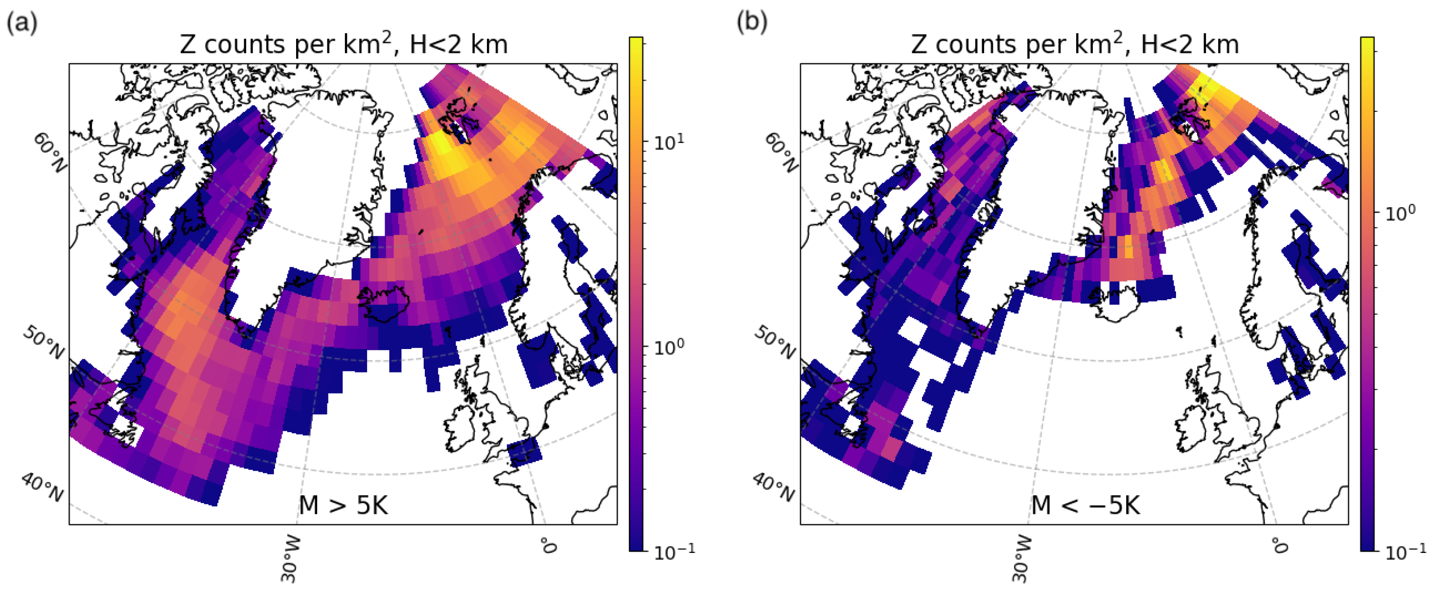The counts shown in the maps in Figure 4 represent the total number of these radar pixels meeting the above criteria, thereby illustrating the geographical distribution of shallow cloud echoes under CAO and non-CAO conditions across the North Atlantic. The radar reflectivity counts were normalized by the area of each 2 × 2 degrees box.

A key contrast between the two maps is the much higher overall frequency of low-level radar echoes (with Z $>-25$ dBZ) during CAO events (left panel) compared to non-CAO events (right panel). The color scales differ by an order of magnitude—with more than 30 counts per ${\mathrm{km}}^2$ in the CAO case versus up to 3 per ${\mathrm{km}}^2$ in the non-CAO case—indicating that shallow, radar-detectable clouds occurred far more frequently under Cold Air Outbreak conditions, as was also noted by [1] in their analysis of the 2CSNOW product. Geographically, CAO-related echoes were especially prevalent around southwestern Greenland, north of Iceland, and in the Norwegian–Barents Sea region, which is consistent with strong cold air advection over relatively warm waters. Notably, the area southwest of Svalbard emerged as a distinct hotspot for CAO events. The pronounced magnitude of this peak compared to the figures in [1] may have resulted either from restrictions on the colorbar used in Figure 4 in their work or from differences in the observational period (their analysis only included data up to December 2010) or a lack of box area normalization.

In contrast, non-CAO events exhibited significantly lower total counts and a more restricted spatial extent. Although notable occurrences could be found east of Greenland and Svalbard, these events were considerably less frequent than those under CAO conditions. This higher occurrence of shallow convective clouds during CAO events not only led to more frequent radar-detectable reflectivity signals in the subpolar North Atlantic, but would also have played a crucial role in the radiative balance of the atmosphere by enhancing the reflection of solar radiation and modulating longwave emissions. Conversely, the less frequent, low-level cloud echoes in non-CAO regimes imply a diminished impact on the regional radiative budget.

3.3.1. Effective Radius

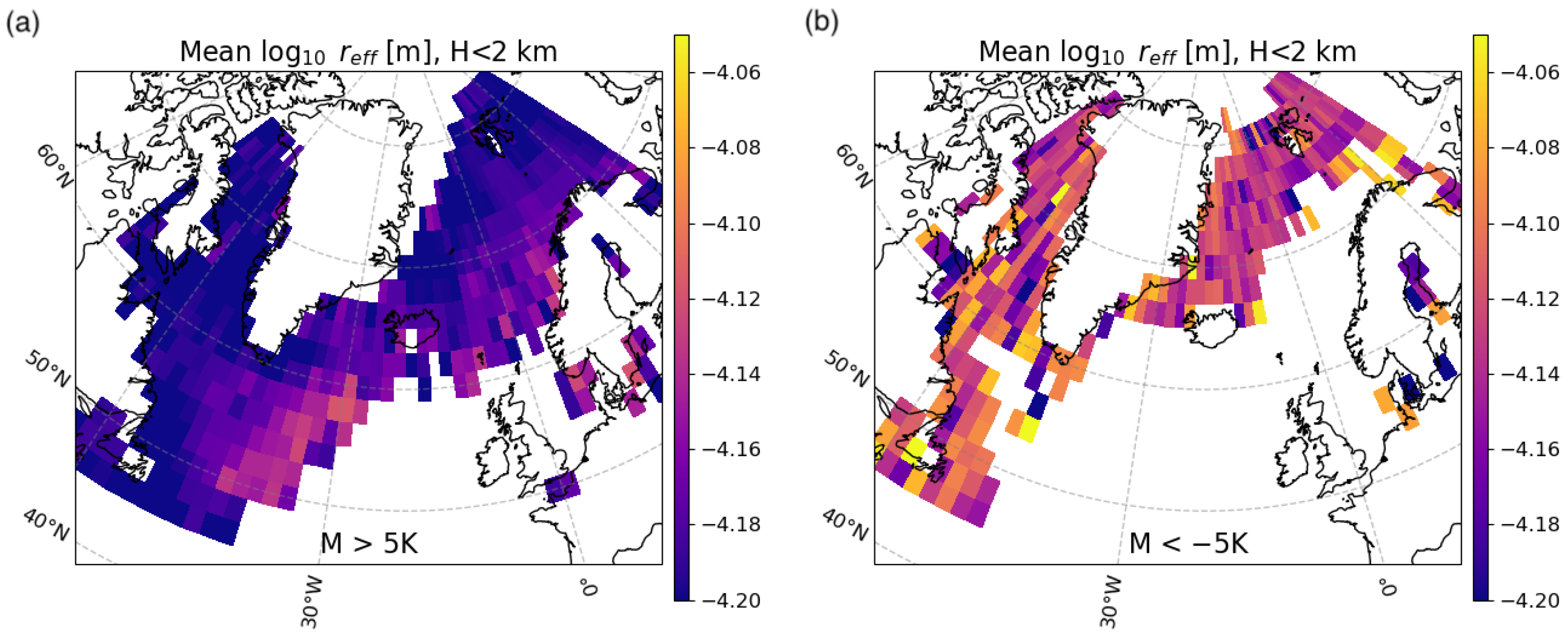
When comparing the mean ${log}_{10}\left(r_{\mathrm{eff}}\right)$ for CAO events and non-CAO events (Figure 5, left and right panels, respectively), a clear contrast emerged across the subpolar North Atlantic. In general, CAO conditions showed more extensive regions of smaller effective radii. In contrast, non-CAO conditions exhibited broader areas of relatively larger effective radii, especially in the vicinity of southwestern Greenland and around the Norwegian–Barents Sea. Notably, southwestern Greenland appeared to be a hotspot for $r_{\mathrm{eff}}$, suggesting that local meteorological factors favored the growth of larger hydrometeors in that region. These differences in spatial patterns reflect the interplay between thermodynamic forcing, aerosol availability, and cloud microphysics, with CAO events generally supporting shallower cloud systems and smaller mean particle sizes compared to non-CAO regimes. Moreover, the observed increase in the effective radius during CAO events away from the sea ice edge was consistent with an increase in the cloud top height and a transition to open-cell convection, highlighting the influence of dynamic cloud structures on cloud microphysical properties.

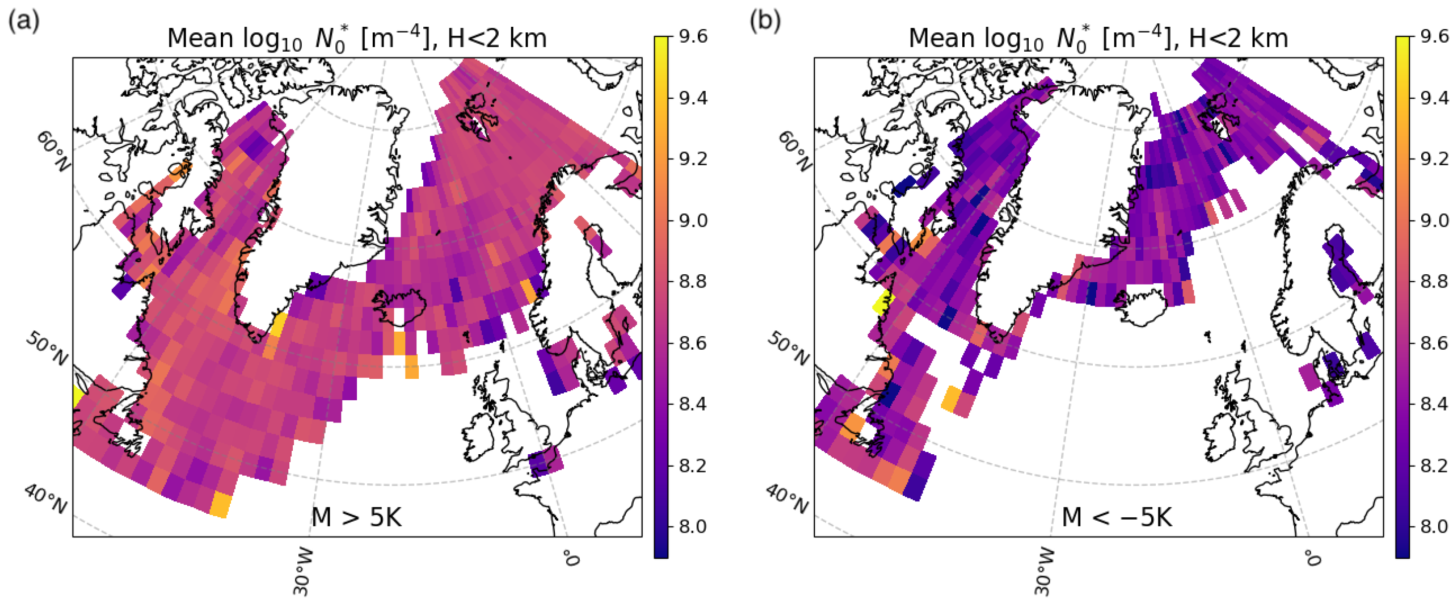
3.3.2. Cloud Particle Concentration

Figure 6a illustrates the mean ${log}_{10}\left(N_0^{*}\right)$ for CAO events, revealing substantially higher particle concentrations across much of the subpolar North Atlantic compared to those for the non-CAO conditions shown in Figure 6b. These higher concentrations coincided with the smaller particle sizes reported earlier, suggesting a regime in which abundant nucleation leads to numerous but relatively small hydrometeors. In contrast, non-CAO events exhibited a lower mean ${log}_{10}\left(N_0^{*}\right)$, indicating fewer but larger particles. Differences in the aerosol and cloud condensation nuclei (CCN) availability could have significantly influenced ice nucleation processes, potentially contributing to the observed differences in particle concentrations ($N_0^{*}$) between CAO and non-CAO cases [10]. Notably, a local minimum in the particle concentration appears northeast of Iceland in the MCAO panel, implying that regional meteorological factors or the aerosol availability may have suppressed cloud particle formation in this specific area. Because the number of observed non-CAO events was much lower, the resulting map is noisier, making it challenging to draw firm conclusions about the spatial patterns of the ice particle number concentration.

3.3.3. Ice Water Content

Although the spatial distribution of the ice water content (IWC) in the lowest 2 km of the atmosphere mirrored that of the effective radius–with regions exhibiting larger effective radii also showing a higher IWC–CAO events typically had a lower IWC compared to non-CAO events. Since CAO events occurred much more frequently than non-CAO snowfall events, it was important to assess which regime contributed more to the total production of ice and snow.

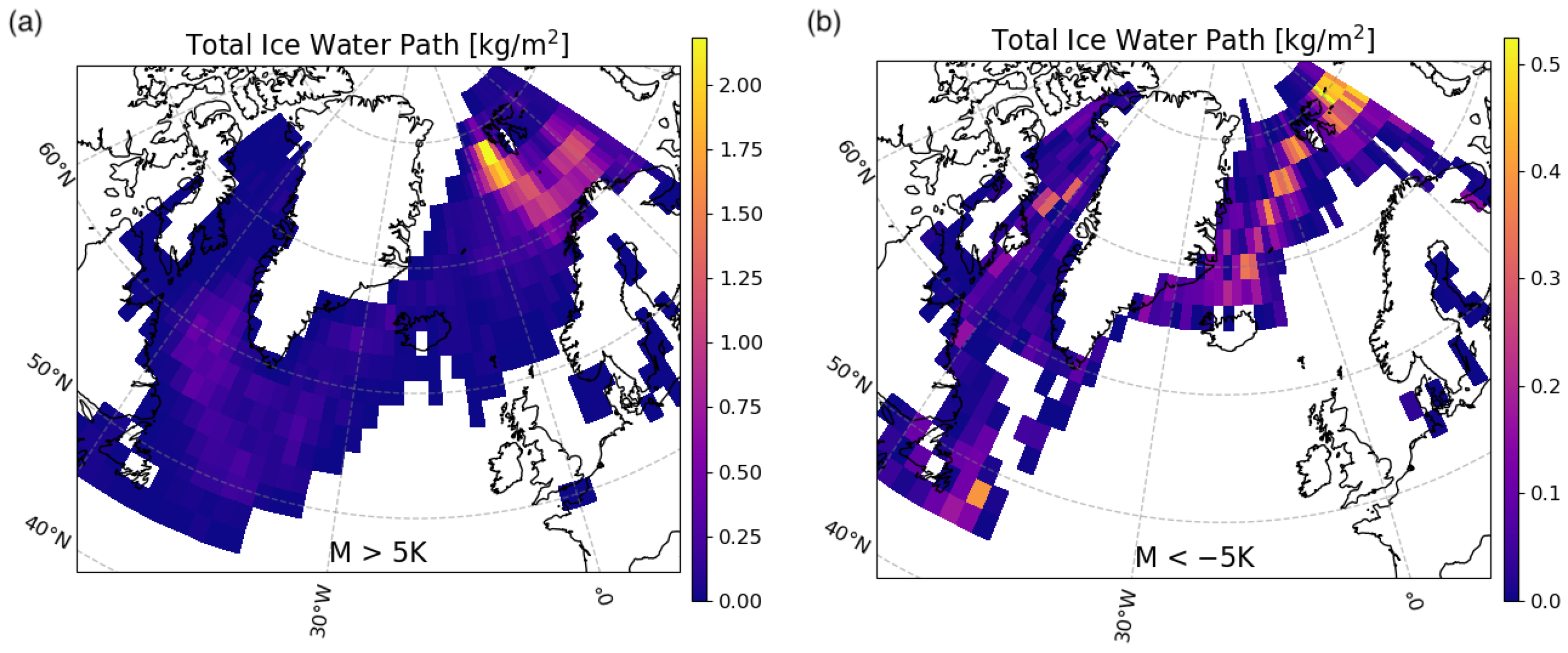
The results of this analysis, presented in Figure 7, provide a quantitative comparison of the cumulative snow and ice contributions from CAO and non-CAO events. Note that these maps serve only as a proxy for comparing CAO and non-CAO conditions, rather than providing the total accumulation in each area, because they rely on the sparse coverage of a radar that passed over the same region only once every 16 days.

The left panel in Figure 7 shows the total ice water path (IWP) for CAO events, highlighting pronounced maxima south of Svalbard and in the vicinity of southwestern Greenland and extending across the Norwegian–Barents Sea region. Values commonly exceeded 1 kg ${\mathrm{m}}^{-2}$, with localized peaks approaching 2 kg ${\mathrm{m}}^{-2}$. In contrast, the right panel depicts non-CAO events, which exhibited a markedly lower total IWP overall, with maximum values of around 0.5 kg ${\mathrm{m}}^{-2}$ east of Svalbard. Although there was still a notable hotspot east of Greenland for non-CAO conditions, the spatial extent and magnitude of these maxima were substantially smaller than those for CAO events. These findings indicate that, despite a lower ice water content at any given time, the frequent occurrence of CAO events led to a substantial integrated ice mass over the analysis period, indicating that CAOs significantly contribute to the total snow and ice production in the subpolar North Atlantic. However, given CloudSat’s limited sampling frequency, cautious interpretation is needed when drawing quantitative conclusions about the absolute dominance of CAO snowfall [1].

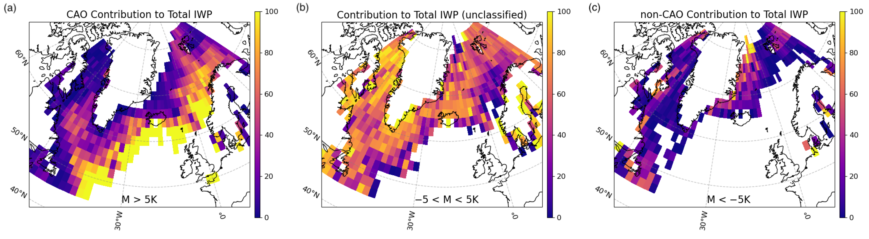
Figure 8 displays the fractional contributions of CAO, non-CAO, and unclassified events to the total observed IWP across the North Atlantic region. Several patterns emerged:

• CAO events: These dominated in the southernmost portion of the analysis domain—particularly along the North American coast—indicating that Cold Air Outbreaks strongly influenced ice production there.
• Unclassified events: Closer to the sea ice edge (e.g., around southern Greenland and parts of the Norwegian Sea), unclassified events accounted for the largest fraction of the IWP. This suggests that intermediate meteorological conditions, neither strong CAOs nor fully non-CAOs, could be quite important where sea ice was present.
• Non-CAO events: Their fractional contribution became significant mainly in the coastal areas east of Greenland, around Svalbard, and near the North American coast. Even though these were not Cold Air Outbreaks, they still produced notable ice in these regions.

Overall, the figure highlights that CAO-driven ice formation was prominent in lower latitudes (south and west), while unclassified conditions dominated closer to the ice edge, and non-CAO conditions made a substantial contribution in more localized coastal zones. The observed increase in the effective radius (Figure 5) and ice water path (Figure 8) with the distance from land or sea ice edges supports the hypothesis introduced earlier (Section 1) that longer fetch lengths enhance the convective depth and snowfall formation processes.

The differences in the snowfall distribution between CAO, unclassified, and non-CAO events illustrated in Figure 7 and Figure 8 reflect distinct underlying meteorological and microphysical conditions:

• CAO events showed the highest cumulative snowfall totals (IWP), primarily concentrated south of Svalbard, around southwestern Greenland, and in the Norwegian–Barents Sea region. This distribution aligned with regions frequently exposed to intense cold air advection over relatively warmer ocean surfaces, promoting persistent shallow convection and snowfall production.
• Unclassified events dominated snowfall closer to the sea ice edge (e.g., around southern Greenland and portions of the Norwegian Sea), where conditions did not distinctly reflect strong CAO nor non-CAO states. These events may have represented transitional or intermediate conditions, potentially including weaker cold air advection scenarios or the mixed influences of synoptic-scale systems and localized convective forcing.
• Non-CAO events exhibited generally lower cumulative snowfall totals but maintained significant contributions near coastal areas east of Greenland, around Svalbard, and along the North American coast in particular. Such a distribution suggests that these snowfall events were primarily associated with synoptic-scale systems like frontal cyclones, which are dynamically forced by large-scale lifting mechanisms and can occasionally produce substantial snowfall.

The distinct spatial patterns and magnitudes observed for these three regimes highlight the variability in the meteorological forcing mechanisms and cloud microphysical processes governing snowfall production across the subpolar North Atlantic. These differences emphasize the importance of classifying snowfall events according to atmospheric stability conditions (M parameter), as each category is associated with fundamentally different cloud processes, snowfall intensities, and spatial distributions.

4. Summary and Conclusions

Marine Cold Air Outbreaks (CAOs) represent a critical component of atmospheric processes in high-latitude regions, influencing cloud formation, snowfall, and turbulent heat exchanges. This study provided new insights into the vertical structure and microphysics of CAO-associated snowfall using active remote sensing data from the A-Train satellite constellation. Specifically, CloudSat–CALIPSO radar–lidar retrievals were used to evaluate the differences between CAO and non-CAO snowfall events.

Our analysis confirmed that CAO snowfall is primarily associated with shallow stratocumulus cloud structures, typically exhibiting cloud top heights below 3 km, as has already been noted by [1]. This contrasts with non-CAO snowfall events, which show deeper cloud systems extending up to 10 km. The ice water content (IWC) in CAOs is generally lower and more narrowly distributed than in non-CAO events, which reflects different microphysical regimes rather than simply a lower precipitation efficiency. The lower IWCs in CAOs are associated with distinct nucleation and growth processes that differ significantly from those in deeper, non-CAO cloud systems [6,11]. The probability density functions of the IWC vertical structure revealed that, while non-CAO snowfall extends across a broader vertical range, CAO snowfall remains tightly confined within the boundary layer.

Clouds embedded within CAOs exhibit distinctive microphysical properties compared to those associated with non-CAO events. Specifically, we found that the ice effective radii and ice water paths increased with the distance from land or sea ice edges, suggesting that longer fetches during CAOs lead to deeper convection and enhanced snowfall production. These findings align with previous research indicating that the initial strength of a CAO has a lasting effect on cloud properties, with differences between clouds in strong and weak events visible over 30 h after the air has left the ice edge [30]. The vertical distribution of the retrieved effective radius ($r_{\mathrm{eff}}$) further illustrated the microphysical distinctions between CAO and non-CAO snowfall. In CAOs, $r_{\mathrm{eff}}$ values were predominantly clustered below 2 km. At those altitudes, retrieved effective radii peaks at 59 μm were distributed for CAO events, compared to a slightly larger peak of 62 μm for non-CAO events. Although the difference in peak values appears modest, the standard deviation of the particle size was notably larger for non-CAO events (18 μm) than for CAO events (15 μm). This broader distribution indicates that larger ice particles occurred more frequently during non-CAO snowfall events. These findings support the notion that CAO snowfall is governed primarily by strong boundary layer inversions, which limit vertical cloud development and constrain ice production, despite the availability of moisture near the ocean surface [7,12].

Our analysis confirmed that the fetch length is a key factor modulating the microphysical properties of CAO clouds; however, the initial atmospheric stability and aerosol–cloud interactions also critically influence the evolution of CAO cloud microphysics and should be considered alongside the fetch length when interpreting snowfall variability [10]. These results underscore the distinct microphysical regimes that differentiate CAO-induced snowfall from other high-latitude precipitation systems and highlight the central role of boundary layer processes in shaping cloud microphysics and snowfall formation. These processes, as documented by recent observational campaigns and modeling studies [7,8,12], offer valuable constraints for improving numerical weather prediction models and climate simulations.

This study is subject to several limitations. First, CloudSat’s temporal sampling frequency (16-day revisit cycle) introduced potential sampling biases, particularly affecting transient snowfall events. Although previous validation (e.g., [21,26]) has indicated the overall reliability of CloudSat retrievals at annual scales, short-lived or localized events may remain underrepresented. Furthermore, the analysis did not incorporate aerosol or cloud condensation nuclei (CCN) data due to dataset constraints, thus excluding aerosol–cloud interactions which could significantly impact ice nucleation processes. Finally, our classification criterion using the widely used MCAO index (M) was practical, but using the threshold value of 5 K remained somewhat subjective and the analysis would benefit from systematic sensitivity testing in future studies.

While CloudSat and CALIPSO data have been invaluable for analyzing cloud microphysics, the recently launched EarthCARE mission [31] is poised to significantly advance this field. In particular, EarthCARE’s synergistic ACM-CAP retrieval [32] will offer a holistic view of atmospheric scenes by simultaneously retrieving the properties of clouds, precipitation, and aerosols. This will facilitate detailed investigations into cloud–aerosol interactions, an important but underexplored aspect in the current study. Additionally, EarthCARE’s cloud profiling radar (CPR) is equipped with Doppler velocity measurements, providing critical insights into vertical air motions and hydrometeor terminal velocities [33], thereby adding a dynamical context that is absent in DARDAR-based retrievals. With an approximate ground footprint of 750 m, EarthCARE’s CPR will also enhance the detection of small-scale cloud structures such as open-cell convection and narrow cloud streaks near the sea ice edge. These capabilities are expected to fill key observational gaps identified in this study. Addressing these limitations through high-resolution, multi-parameter satellite retrievals, combined with aerosol measurements and targeted field campaigns, will be essential for improving the representation of high-latitude cloud processes in weather and climate models.