Analysis of Spatio-Temporal Variation Characteristics of Air Pollutants in Zaozhuang China from 2018 to 2022

Abstract

Based on the air-quality monitoring data of Zaozhuang City from 2018 to 2022, this study systematically analyzed the spatio-temporal variation characteristics of multiple pollutants by comprehensively applying Kriging interpolation, time-series decomposition, wavelet transform, and DBSCAN spatial clustering methods. The key findings include: (1) Overall, air pollutant concentrations in Zaozhuang decrease from 2018 to 2022, with NO₂, SO₂, PM_2.5, and PM₁₀ concentrations declining by 17.3%, 52.2%, 28.9%, and 33.6%, respectively. However, O₃ concentration increases by 2.5% in 2022 compared to 2018. Seasonally, SO₂, PM_2.5, and PM₁₀ concentrations are the highest in winter and lowest in summer, while CO, NO₂, and O₃ follow a winter > autumn > spring > summer pattern. Weekly variations show that daily average concentrations of CO, NO₂, SO₂, PM_2.5, and PM₁₀ peak on Mondays, with concentrations slightly higher on weekdays than weekends. (2) Spatially, CO, NO₂, PM_2.5, and PM₁₀ concentrations are higher in the southern region, while O₃ and SO₂ concentrations are elevated in Shizhong District, Xuecheng District, and Tengzhou City. (3) Correlation analysis reveals that meteorological parameters, such as precipitation, significantly influence pollutant concentrations, with precipitation playing a role in reducing pollutant levels. This study highlights the effectiveness of the Kriging method in analyzing the complex spatio-temporal dynamics of air pollutants, offering valuable insights for environmental policy and urban planning.

1. Introduction

With the increase in population, there has been a rapid development of urbanization and industrialization, and, while human beings have achieved economic development, they have also added great pressure to the ecological environment and caused environmental pollution, resource depletion, land desertification, and other consequences [1,2,3,4,5]. Environmental pollution has become a pressing global issue, severely threatening human health and ecosystems [6]. Environmental problems caused by air pollution have appeared, which has seriously affected the normal production and health of humans [7,8,9,10]. The lives of urban residents are directly affected by air quality. The related research on the urban atmospheric environment has gradually attracted the attention of scholars [11,12,13]. Therefore, it is of great theoretical significance to study the variation law of urban air pollutants.

Zaozhuang (116°48’ E-117°49′ E, 34°27′–35°19′) is located on the border area of the Jiangsu and Shandong Provinces, is the southern gate of Shandong Province, and is also one of the 20 prefecture-level cities in the Huaihai Economic Zone. The total area is 4564 square kilometers, accounting for 2.97% of the total area of Shandong Province. Zaozhuang City is located in the southern region with low mountains and hills, in the central-south of Shandong Province, which is part of the Huang-Huai alluvial plain. The terrain is high in the north and low in the south, and high in the east and low in the west. According to the 7th National census bulletin of Zaozhuang City, the city’s population is 3.855 million. From the perspective of Zaozhuang’s industrial structure, the comparative advantage of abundant labor resources has driven the rapid development of labor-intensive industries, such as textiles and clothing. The characteristics of the low cost of production factors and rich resources have created industries dominated by coal, cement, and chemicals. At present, Zaozhuang City vigorously promotes the strategy of creating an “industrial strong city”. However, Zaozhuang has not been able to solve the problems of unreasonable industrial structures and extensive developments, and the city’s heavy chemical industries, such as thermal power, cement, chemical, and coke production, account for a large proportion of the industry. These industries not only create economic value, but also increase the emissions of pollutants and contribute very much to air pollution. The main pollutant in Zaozhuang is suspended particulate matter, that is, dust pollution [14]. The sources of dust include coal burning dust and industrial dust, as well as mining, construction dust, and vehicle dust. At present, the air quality of Zaozhuang ranks low in the country, and the pollution is severe.

Liu et al. (2018) [15] studied the temporal and spatial distribution characteristics and correlation of PM_2.5 in urban agglomerations in China’s industrial bases, and the results showed that the seasonal variation characteristics of PM_2.5 were generally presented as winter > autumn > spring > summer. The pollution level of Beijing–Tianjin–Tangshan is higher than that of the other three industrial bases. Ma et al. (2018) studied the spatial and temporal distribution of air pollutants in the north and south of China, and the results showed that the heavily polluted areas were mainly distributed in the Bohai Rim, the Yangtze River Delta, and the northwest of China, and the concentration of air pollutants in the south and the north had obvious monthly changes [16]. Chen et al. (2018) studied the distribution characteristics of atmospheric particles in the cold and warm seasons over the Chinese mainland, and the results showed that the air pollution in most areas was more serious in the cold season than in the warm season [17]. Zang et al. (2015) studied the spatial and temporal distribution characteristics of the main air pollutants in China, and the results showed that the air pollutants showed obvious regional distribution characteristics, and the general trend of concentration was lower in the southern region than in the northern region [18].

Previous studies on air quality or air pollution have focused more on developed city clusters or key regions. For example, Li et al. [19] studied the long-term air pollution characteristics of mega-mountain cities in the Chengdu–Chongqing economic circle. Zhang et al. [20] compared and analyzed the seasonal and diurnal variations in the composition and concentration of VOCs in a typical chemical industrial development zone in eastern China. Li [21] analyzed the structural characteristics of air pollution in “2 + 26” cities from 2017 to 2021 by performing a social network analysis. Guan et al. [22] studied the time variation characteristics of ozone pollution and the influence of meteorological factors in the Pudong new area of Shanghai. Wang et al. [23] studied the distribution characteristics of air pollutants under different pollution levels in Cangzhou City. Most studies focus on the analysis of a single pollutant or a specific area. For a city like Zaozhuang, which has a complex industrial layout and topographic conditions, there are relatively few studies on the systematic spatio-temporal variation characteristics. Our research comprehensively analyzed the spatio-temporal variation characteristics of various air pollutants in Zaozhuang City from 2018 to 2022 through multiple methods, filling this research gap. At present, the research on air pollution in Zaozhuang City is not deep and comprehensive enough. Especially, the basic research of air pollution in Zaozhuang is not enough. In this study, the long-term observation data of air pollutants are used for in-depth analysis in order to better understand the air pollution situation in Zaozhuang City. The Kriging interpolation method not only considers the spatial distance between the predicted points and the adjacent sampling points, but also considers the position relationship. At present, Kriging interpolation is widely used for the analysis of air pollutants. In this study, the daily concentration data of six basic pollutants were processed to obtain the annual, seasonal, and monthly mean values, and their spatial distribution was plotted using the Kriging interpolation method and the relationship between the pollutant concentration and meteorological conditions through various statistical analysis methods.

Based on the daily observation data of six kinds of air pollutants and meteorological observation data from 2018 to 2022, this study analyzed the annual, monthly, and weekly variation characteristics of air pollutants in Zaozhuang City. Air pollutant data from 26 monitoring stations in Zaozhuang and surrounding areas were used to study spatial characteristics by using the Kriging method. Finally, the correlation between six kinds of pollutants and meteorological parameters was explored.

2. Data and Methods

2.1. Data Preprocessing

In this study, the daily concentration data of atmospheric pollutants (O₃, NO₂, CO, SO₂, PM_2.5, and PM₁₀) in Zaozhuang City from 2018 to 2022 provided by the National Environmental Monitoring Station (as shown in Figure 1) were used. Meteorological data were obtained from China’s ground meteorological monitoring stations, including the main meteorological parameters of temperature (°C), pressure (hPa), dew point (°C), wind direction and speed (m/s), cloud cover (%), and precipitation (mm). From the perspective of intra-seasonal variation, this study explored the influence of selected meteorological parameters on the change in pollutant concentration in Zaozhuang City from 2018 to 2022.

The collection of original data may have been affected by various factors, such as abnormal monitoring station devices, improper operations, and database disk faults. Therefore, it was necessary to pre-process the atmospheric pollutant concentration data and meteorological parameter data obtained. A series of methods were needed to remove duplicates, fill in gaps, and replace and delete the original observation data. The methods mainly included: (1) Filtering the data with obvious errors. For example, for PM_2.5 concentration, negative values are obviously wrong, and for relative humidity data, data less than 0 or greater than 1 are obviously wrong. (2) Filling in the data when missing. For the period missing data, the observed data have three trends of rising, falling, and smoothing. For missing data with an upward or downward trend, calculate the difference of known observations at both ends of the data missing period and fill them in by arithmetic difference. If they are missing data with a smooth trend, they are filled with the mean value of the remaining observations. This filling method takes into account the overall characteristics of the information before and after the time-series data in order to minimize the impact of the occurrence of outliers on the later training and verification of the model. (3) Removing the data with large deviations. Due to natural factors or hardware equipment and other factors, the collected air pollution data may deviate from the normal value range. These excessively biased data will affect the accuracy of the subsequent research results, so it is necessary to identify and filter such data using the 3σ principles of the Gaussian distribution.

Finally, the Pearson correlation between atmospheric pollutants and meteorological parameters in each season was calculated separately.

2.2. Kriging Interpolation Method

Because of the uneven spatial distribution of the sampling points, it was necessary to carry out spatial interpolation to obtain the distribution characteristics of the whole data in the region. The Kriging method [24,25,26] is a geostatistical interpolation technique that considers both the distance and the degree of variation between known data points when estimating values in unknown areas. Based on the theoretical analysis of regionalized variables, this method uses the semi-variance function as a tool to estimate the value of regionalized variables in a finite region. At present, Kriging interpolation is widely used for the analysis of air pollutants. First, a distance range with some influence is determined for the point value to be interpolated. The sample points in this range are then used to estimate the attribute values of the points to be interpolated. It considers not only the interrelationship between the position of the point to be estimated and the position of the known data, but also the spatial correlation of the variables. By processing the daily concentration data of 6 basic pollutants, the annual, seasonal, and monthly mean values were obtained, and their spatial distribution was plotted using the Kriging interpolation method.

In this study, the Kriging interpolation method in ArcGIS 10.8 software was used to realize the spatial distribution characteristics of air pollutants. SPSS 22.0 software was used to analyze the correlation between atmospheric pollutant concentration and meteorological factors. Based on the above data, this study explored the spatio-temporal variation rules and influencing factors of air pollutants in Zaozhuang City. The annual, quarterly, monthly, weekly, and daily changes were analyzed on the time scale. The Kriging interpolation method was used to study the spatial distribution characteristics of air pollutant concentrations based on the observation data of pollutant monitoring stations in Zaozhuang City and three neighboring cities: Linyi, Jining, and Xuzhou.

2.3. Mann–Kendall Test and Sen’s Slopes

The Mann–Kendall test is a non-parametric statistical method used to detect the trend of time series, which is widely used in environmental science, hydrology, meteorology, and other fields to judge whether there is an obvious trend and the direction of the trend in a time-series data set [27,28,29]. S represents an increase or decrease in the time-series trend.

$$S={\sum }_{j=1}^{n-1}{\sum }_{k=j+1}^{n}s(X_k-X_j)$$

(1)

where $X_j$ and $X_k$ are the corresponding measured values in years j and k, and k > j.

Statistic Z of the Mann–Kendall test represents the strength of the trend present in the data series:

$$Z={\displaystyle \frac{S}{\sqrt{V\left(S\right)}}}$$

(2)

where Z is the statistic of a normal distribution and V(S) is the variance. If ∣Z∣ ≥ $Z_{1-a/2}$, there is a clear upward or downward trend in the time-series data at a given ɑ confidence level. ∣Z∣ ≥ 1.96 and ∣Z∣ ≥ 2.58 indicate that they pass the significance test with 95% and 99% confidence values, respectively.

Sen’s slopes method can reduce or avoid the influence of missing data and anomalies on the statistical results. Based on a certain significance level, ɑ, the statistical test was carried out to obtain the numerical interval of the rate of change. The median value was used to determine the trend and extent of the time-series change. The slope formula is:

$$S_{ij}=M\left[{\displaystyle \frac{X_j-X_i}{j-i}}\right]$$

(3)

where $X_i$ and $X_j$ are sequence values at the i and j moments, respectively. 1 < I < j < n, where n is the length of the sequence.

3. Results and Discussion

3.1. Spatio-Temporal Variation Characteristics

3.1.1. Basic Status of Air Pollutants

In 2022, the concentration of air pollutants in Zaozhuang exceeded the secondary limits of the national ambient air-quality standards, as shown in

Table 1. Statistics of air pollutants exceeding the Grade II national standards for air quality in Zaozhuang City in 2022.

Category	Exceedance Days	Total Days	Over-Standard Rate/%
O3	14	365	3.8
CO	0	365	-
NO2	0	365	-
SO2	0	365	-
PM2.5	42	365	11.5
PM10	30	365	8.2

. The monthly proportion of pollutants exceeding the standard in Zaozhuang City in 2022 is shown in Figure 2. In 2022, the concentration of O₃ in Zaozhuang exceeded the standard (daily concentration > 200 μg/m³) for a total of 14 days, and the exceeded rate was 3.8%. From the monthly change point of view, the ozone concentration exceeded the standard for 11 days in June, and the exceeded rate was 36.7%. In May and September, the O₃ concentration exceeded the standard for 2 days and 1 day, and the exceeded rates were 6.5% and 3.3%, respectively. From the points of view of the duration and intensity of the pollution process, the ozone concentration in June was concentrated and significantly higher than in other months. Moreover, there were 3 days in June when the ozone concentration was higher than 240 µg/m³ (more than 20% of the standard), and the highest value reached 250 µg/m³, significantly higher than the other months. In 2022, Zaozhuang’s PM_2.5 concentration exceeded the standard for 41 days (daily concentration > 75 µg/m³), and the exceedance rate was 11.5%. In terms of the monthly changes, the number of days exceeding the standard was concentrated in January and December. In January and December, the number of days exceeding the standard was 19 days and 13 days, and the rate of exceeding the standard was 63.3% and 43.3%, respectively. In 2022, there were 31 days with a PM_2.5 concentration above 90 µg/m³ (more than 20% of the standard), accounting for 93.5% in January and December, and the highest value reached 175 µg/m³. In 2022, the concentration of PM₁₀ in Zaozhuang exceeded the standard (daily concentration > 150 µg/m³) for 30 days, and the exceeded rate was 8.2%. In terms of the monthly changes, in January, March, and April, the standard was exceeded for 10, 7, and 1 days, respectively, and the exceeded rates were 32.2%, 22.6% and 3.3%, respectively. A total of 13 days in 2022 saw PM₁₀ concentrations above 180 µg/m³ (more than 20% of the standard), with a maximum of 275 µg/m³.

The concentrations of NO₂, SO₂, CO, and other pollutants decreased after the implementation of key pollution control and industrial upgrading measures. In 2022, the concentrations of NO₂, SO₂, and CO in Zaozhuang will be stable and reach the standard.

3.1.2. Interannual Variation Characteristics

Figure 3 shows the change trend of the annual average concentration of various pollutants in Zaozhuang from 2018 to 2022. As can be seen from the figure, the interannual change in NO₂, SO₂, PM_2.5, and PM₁₀ concentration shows a downward trend, which decreases by 17.3%, 52.2%, 28.9%, and 33.6%, respectively, from 2018 to 2022. The average O₃ concentration in 2018–2021 showed a downward trend, but the average annual ozone concentration in 2022 increased by 2.5% compared with 2018.

3.1.3. Seasonal Variation Characteristics

The seasonal changes in various pollutant concentrations in Zaozhuang City from 2018 to 2022 are shown in Figure 4 and

Table 2. Mean atmospheric pollutant concentration ± standard deviation for the four seasons in 2018–2022 (µg/m³).

Pollutant	Spring	Summer	Autumn	Winter	Annual Mean
O3	126.3 ± 33.5	146.5 ± 47.0	114.6 ± 41.3	74.3 ± 18.8	115.6 ± 45.1
CO	0.554 ± 0.166	0.569 ± 0.128	0.648 ± 0.220	0.858 ± 0.257	0.631 ± 0.245
NO2	28.2 ± 9.3	17.9 ± 4.7	32.8 ± 14.1	38.7 ± 14.9	28.3 ± 13.6
SO2	14.2 ± 4.0	11.1 ± 3.0	14.2 ± 4.9	16.6 ± 5.2	14.0 ± 4.8
PM2.5	41.8 ± 20.5	24.2 ± 9.6	39.8 ± 25.7	70.6 ± 35.4	44.0 ± 29.7
PM10	104.1 ± 85.8	48.9 ± 23.0	77.4 ± 41.6	121.9 ± 49.7	88.0 ± 61.5

. The O₃ concentration in Zaozhuang City showed obvious seasonal changes, and the concentration changed from high to low in summer, spring, autumn, and winter. The high temperature and strong solar radiation in summer are conducive to the production of O₃. The seasonal variation om O₃ is obviously related to the variation in meteorological conditions, such as temperature and solar illumination. In winter, the temperature is low and the sunshine duration is significantly less than that in the previous three seasons, which is not conducive to the photochemical reaction needed to produce O₃. In winter, the weather is rainy, snowy, and windy, which is conducive to the diffusion of pollutants. In summer, the temperature is high and the light is strong. Therefore, O₃ is the most polluted in summer and the least polluted in winter. The CO concentration reached the maximum value of 2.6 µg/m³ in winter, and the lowest concentration was 0.1 µg/m³ in summer.

As one of the O₃ precursors, the concentration of NO₂ decreases from high to low in the order of winter, autumn, spring, and summer. As can be seen from Table 2, the highest winter level (38.7 ± 14.9) is 10 µg/m³ higher than the lowest summer value (28.2 ± 9.3), and the concentrations in spring and autumn are 28.2 ± 9.3 µg/m³ and 32.8 ± 14.1 µg/m³, respectively. The concentration of SO₂ was the highest in winter, with an average of 16.6 ± 5.2 µg/m³. The seasonal variation in PM_2.5 concentration and PM₁₀ concentration is consistent, showing obvious seasonal variation characteristics of high in winter, low in summer, and medium in spring and autumn. It shows that, under the influence of meteorological conditions and other factors, the seasonal variation in homologous PM₁₀ and PM_2.5 is consistent. On the one hand, the increase in particulate matter concentration in winter is due to the increase in central heating and pollutant emissions in Zaozhuang in winter. On the other hand, the winter atmosphere is static and stable, which easily causes the accumulation of pollutants.

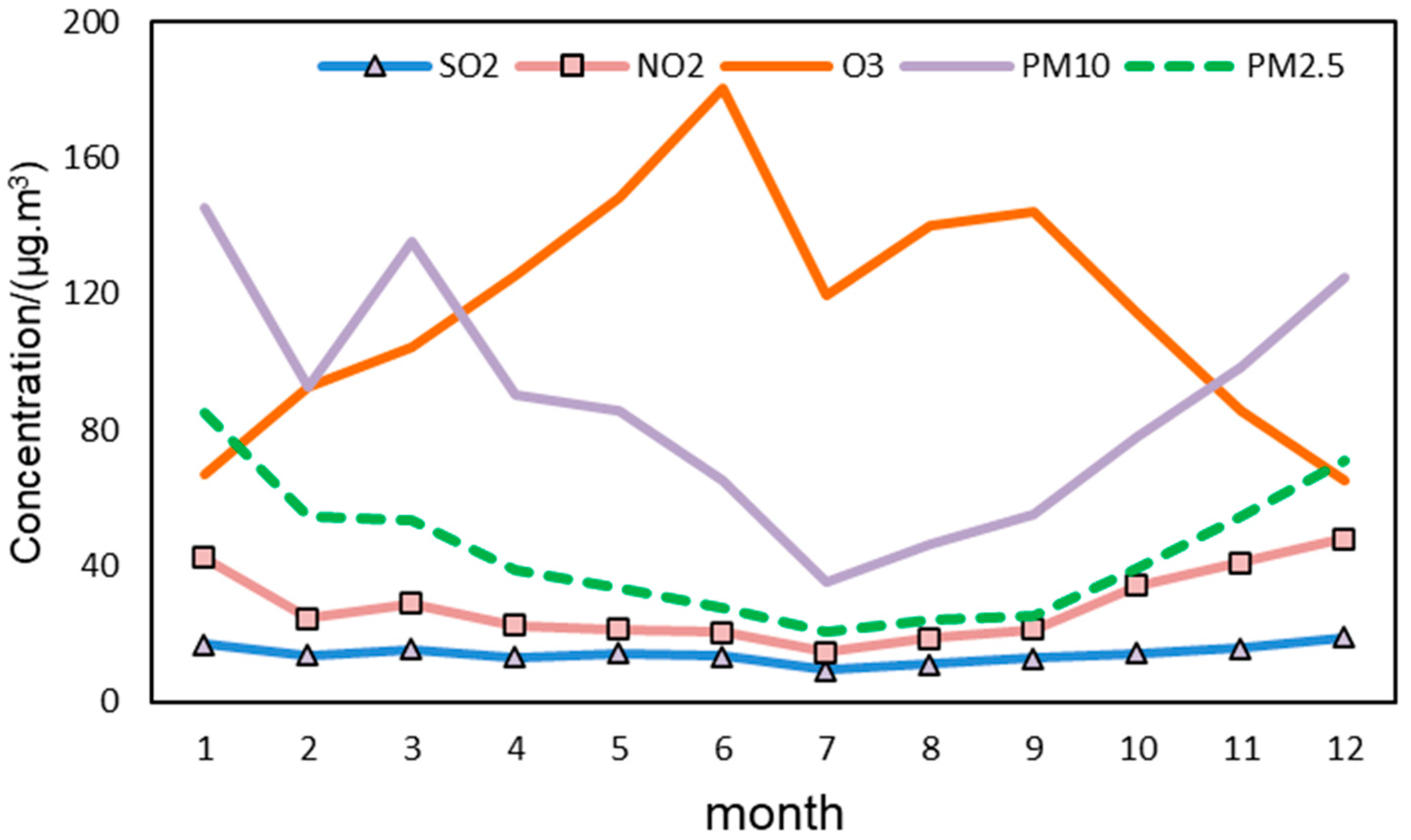
3.1.4. Monthly Variation Characteristics

Figure 5 shows the monthly change trend of various pollutants in Zaozhuang City from 2018 to 2022. As shown in the figure, except for O₃, all pollutants are consistent and present a U-shaped change. December and January are the months with high concentrations, while June, July, August, and September are the months with low concentrations. The average monthly concentration of O₃ shows a bimodal variation, with peaks appearing in June and September. In June, the temperature and sunshine duration increased, and the photochemical reaction was enhanced, which was conducive to the formation and accumulation of O₃, and the ozone concentration increased significantly.

PM_2.5 and PM₁₀ concentrations peaked in January at 85.0 µg/m³ and 145.2 µg/m³, respectively. In January, a long period and a wide range of quiet and stable weather resulted in poor air mobility and difficult diffusion of pollutants, leading to a continued rise in PM_2.5 concentrations. At the same time, due to the large temperature variation, the emissions of domestic sources, such as coal sources and transportation sources, which are closely related to heating and travel, also increased correspondingly, further aggravating air pollution. The lowest values were reached in July, with minimum values of 20.6 µg/m³ and 35.5 µg/m³. The monthly variation trend of O₃ concentration is different from other concentrations, with the highest value appearing in June (180.6 µg/m³) and the lowest value appearing in December (65.0 µg/m³), showing a trend of high summer and low winter in general.

3.1.5. Weekly Variation Characteristics

Table 3. Weekly change in pollutants from 2018 to 2022 in Zaozhuang (µg/m³).

Pollutant	Monday	Tuesday	Wednesday	Thursday	Friday	Saturday	Sunday	Max	Min
O3	114.8	116.6	122.8	123.3	125.6	117.2	121.2	114.8 (Monday)	125.6 (Friday)
CO	0.714	0.712	0.7	0.692	0.7	0.685	0.689	0.685 (Saturday)	0.714 (Monday)
NO2	29.0	27.9	27.7	27.2	27.8	27.3	27.4	27.2 (Wednesday)	29.0 (Monday)
SO2	14.5	13.7	14.1	14.3	14.0	13.8	14.4	13.7 (Tuesday)	14.5 (Monday)
PM2.5	44.6	42.5	40.7	37.6	40.0	39.0	39.1	37.6 (Thursday)	44.6 (Monday)
PM10	83.8	83.3	82.5	73.4	75.8	75.2	75.1	73.4 (Thursday)	83.8 (Monday)

shows the weekly variation characteristics of various pollutants in Zaozhuang City from 2018 to 2022. As can be seen from the table, the maximum daily average concentrations of CO, NO₂, SO₂, PM_2.5, and PM₁₀ all appear on Monday, reaching 0.714 µg/m³, 29.0 µg/m³, 14.5 µg/m³, 44.6 µg/m³, and 83.8 µg/m³ respectively.

The concentration changes in various pollutants in Zaozhuang City on weekdays and weekends in 2022 are shown in Figure 6. As can be seen from the figure, all pollutants, except O₃, are basically higher on weekdays than on weekends, mainly because more pollutants are emitted by traffic on weekdays [30,31].

3.1.6. The Result of the Mann–Kendall Test and the Detection of Extreme Pollution Events

PM_2.5 concentration showed a significant seasonal decline, and all seasons passed the significance test (p < 0.01), indicating that the pollution prevention measures implemented in recent years achieved good results in different seasons. Among them, spring showed the most significant improvement trend (Z = −8.67, p = 4.50 × 10⁻¹⁸). The rate of decline was the greatest in winter. Summer and autumn also showed a significant downward trend. The monthly variation in PM_2.5 concentration showed obvious differentiation. The most significant downward trend was observed in February (slope of −0.264, p = 6.46 × 10⁻⁵). A significant downward trend was observed for three consecutive months from April to June (slope range from −0.16 to −0.12; p < 1.09 × 10⁻⁶). It is worth noting that there is a steep downward trend in November (slope of −0.25, p = 8.92 × 10⁻⁶). In contrast, the improvement trends in August (p = 0.073) and December (p = 0.627) did not reach significant levels. The daily variation trend of PM_2.5 concentration showed obvious cyclical fluctuation characteristics. The first day of each month shows the most significant downward trend (slope of −0.714, p = 0.0017). The mid-month period (16–17, 21–22) formed the second significant decline interval, with the greatest decline on 21 (slope −0.624, p = 0.0005). It is worth noting that the end of the month 28–29 also showed a significant improvement (slope of −0.415 to −0.526, p < 0.033).

The O₃ concentration showed significant seasonal differences. Winter shows the strongest upward trend (Z = 4.95, p = 7.52 × 10⁻⁷, slope = 0.036). In summer, there was a significant downward trend (Z = −3.41, p = 0.00064, slope = −0.061). The change trend in spring and autumn was not significant (p > 0.05), but it still showed a slight upward trend in spring (slope = 0.020). O₃ concentration showed the most significant upward trend in December (Z = 6.99, p = 2.83 × 10⁻¹², slope = 0.156). It also showed a significant increase from January to February (p < 0.002). O₃ concentration decreased significantly in July (Z = −2.54, p = 0.011, slope of −0.197). The diurnal trend of O₃ concentration was not significant, with p > 0.05 on most days.

PM₁₀ concentration showed an extremely significant downward trend in all seasons throughout the year (p < 1.13 × 10⁻⁸). The decline was the greatest in spring (slope = −0.125), and the statistical significance was the strongest (Z = −8.82, p = 1.13 × 10⁻¹⁸). Summer has the next-largest decline (slope = −0.087). Winter (slope = −0.121) and autumn (slope = −0.089) have similar declines. From the perspective of the monthly variation trend, except for August, September, and December, the other months showed a significant decline (p < 0.01). The steepest decline occurred in February (slope = −0.538). From the diurnal variations in PM10 concentration, it generally improved throughout the month. Among them, 29 days showed a downward trend (93.5%). The significant level was at 21 days (p < 0.05).

The overall trend of the seasonal variation in SO₂ concentration was obvious. The decrease was the greatest in spring (slope −0.0198, p = 2.41 × 10⁻²⁰) and had the greatest in statistical significance (Z = −9.24). Winter has the second-largest decline (slope −0.0199, p = 6.80 × 10⁻¹⁴). There was relatively little improvement in autumn and summer. The concentration of SO₂ decreased significantly from January to April and from October to November (p < 0.01). The change in other months is not significant. SO₂ concentration generally improved throughout the month. It showed a downward trend over 30 days, accounting for 96.8%. The significant level was reached in 17 days (p < 0.05).

NO₂ concentration showed a downward trend in all seasons throughout the year. The decrease was greatest in spring (slope = −0.0272, p = 8.67 × 10⁻¹⁹), and the statistical significance was the strongest (Z = −8.85). Summer has the second-largest decline (slope = −0.0115, p = 1.13 × 10⁻⁹). The decrease is similar but less significant in winter and autumn. Except for August, September, and December, NO₂ concentration in other months showed a downward trend (p < 0.01). NO₂ generally improved throughout the month. A total of 29 days showed a downward trend, accounting for 93.5%. The significant level was reached in 7 days for the whole month (p < 0.05).

The decrease in CO concentration in spring was the largest (slope of −0.00040, p = 2.05 × 10⁻¹³), and the statistical significance was the strongest (Z = −7.35). Winter has the second-largest decline (slope of −0.00052, p = 1.03 × 10⁻⁶). There is an upward trend in autumn. CO concentration decreased significantly in January, February, March, May, June, and July. The biggest drop was in February (slope = −0.00241). The change in other months is not significant. There was no significant change in CO concentration on most days of the month (p > 0.05).

We used four outlier detection methods to examine abnormal pollution events. The first one is the interquartile range method, which is based on the quantile characteristics of the data and determines the normal value range by calculating the interquartile range. Exceeding this range is regarded as an exception. The second one is the median absolute deviation method, which uses the median as the central trend measure and constructs the anomaly judgment criterion by calculating the median of the absolute deviation. The third one is the standard fraction method. Based on the assumption of a normal distribution, it calculates the standard deviation distance between the data points and the mean. The fourth one is the percentile method, which directly defines extreme percentiles as the threshold boundary. A “Confirmed Outlier” is only considered if at least two methods simultaneously detect an exception.

The statistical results of extreme pollution events of PM_2.5 are shown in

Table 4. Statistics of extreme pollution events of PM2.5 from 2018 to 2022 (μg/m³).

Year	Number of Events	Average Value	Maximum Value	Median Value
2018	8	208.5	249	208.5
2019	6	199	242	192
2020	3	200	205	203
2021	1	201	201	201

. Extreme pollution incidents show a significant downward trend. The frequency of events sharply declines from eight in 2018 to just one in 2021, a decrease of 87.5%, with an average annual reduction of approximately 42%.

3.1.7. Spatial Distribution Characteristics

According to the observation data of 6 monitoring stations in Zaozhuang and 20 monitoring stations in Linyi, Jining, and Xuzhou in 2022, the spatial distribution of various pollutants in Zaozhuang in 2022 was obtained by applying the Kriging interpolation method, as shown in Figure 7.

As shown in Figure 7, the spatial distribution of various air pollutants in Zaozhuang City in 2022 presents certain differences. The high concentration of SO₂ was distributed in Shizhong District, Xuecheng District, and Tengzhou City. The possible reason is that these areas are the most developed and industrialized areas in Zaozhuang City. Taierzhuang District is a key tourism area in Zaozhuang City, and there are few industrial enterprises in the area, so the concentration of SO₂ is low. The spatial distribution characteristics of NO₂, CO, PM_2.5, and PM₁₀ are basically the same, that is, they gradually decrease from the south to the north, and the lowest values mostly appear in the Shanting area. The main reason is that Shanting District is mainly mountainous. It is in a newly developed state, with a better green ecological environment, and has a lower population and less traffic. The highest concentrations of NO₂, PM_2.5, and PM₁₀ were concentrated in the central district and its surrounding areas. The possible reason is that the mining area and the thermal power industry are concentrated in Tengzhou City. The cement industry, which affects the concentration of nitrogen oxides, is mainly distributed in the Shizhong District. In addition, Shizhong District and Tengzhou City have a large population density and developed transportation. Therefore, the emissions of automobile exhaust and domestic pollution are higher, which leads to increases in PM_2.5 and PM₁₀ concentrations.

The Density-Based Spatial Clustering of Applications with Noise (DBSCAN) clustering method was adopted for spatial patterns of PM_2.5 and O₃ based on six observation stations in Zaozhuang City. The analysis result based on DBSCAN is shown in Figure 8 and

Table 5. Statistical analysis results of PM_2.5 and O₃ based on DBSCAN.

Station ID	Station Name	DBSCAN Group	Geographic Coordinates	PM2.5 (µg/m3)	O3 (µg/m3)
S1	Taierzhuang	0 (noise)	(34.5578, 117.7276)	67.89	77.70
S2	Shanting	0 (noise)	(35.0992, 117.4518)	55.89	89.06
S3	Yicheng	1	(34.7745, 117.5852)	63.32	81.66
S4	Shizhong	1	(34.8438, 117.558)	68.71	83.45
S5	Shihuanbaoju	1	(34.8103, 117.3152)	62.71	81.96
S6	Xuecheng	1	(34.7837, 117.2852)	64.10	81.58

. The PM_2.5 DBSCAN algorithm identified one core cluster (Cluster 1) containing four monitoring stations (S3–S6) and two noise points (S1–S2) based on spatial proximity analysis. The core cluster (S3–S6) exhibits tight geographical cohesion, with an average inter-station distance of 9.2 km, falling within the defined neighborhood radius (eps = 11 km). Noise points S1 and S2 were isolated 18.7 km and 32.4 km, respectively, from their nearest neighbors, exceeding the density threshold. The DBSCAN analysis revealed statistically significant spatial clustering (p < 0.05), with 66.7% of stations forming a cohesive pollution plume (Cluster 1: 64.7 ± 2.5 µg/m³).

The cluster analysis results of O₃ monitoring data based on DBSCAN show that monitoring sites are clearly divided into two categories: core Cluster 1 and noise points. The core cluster consists of four sites, S3, S4, S5, and S6, which are geographically closely clustered (less than 10 km away from each other) and have highly consistent O₃ concentration levels (81.6–83.4 µg/m³), indicating stable regional ozone pollution in the region, possibly due to large-scale meteorological conditions or regional transport. Two sites (S1 and S2) were identified as noise points with significant spatial isolation: S1 is 18.7 km from the nearest site and has an ozone concentration of 77.7 µg/m³; S2 is 32.4 km from the nearest site but has an ozone concentration of 89.1 µg/m³, significantly above the regional average. The results are verified by the parameter sensitivity test, and the results are robust. From the perspective of environmental management, it is recommended to implement coordinated prevention and control in the core cluster area and focus on the abnormal spot (S2) to improve the ozone pollution control strategy.

3.2. Influencing Factors

3.2.1. Analysis of Meteorological Parameters

Meteorological parameters are one of the main influencing factors of air pollutants, and the relationship between them also changes with the seasons. The statistical results of the correlation between pollutants and meteorological parameters in Zaozhuang in the four seasons of in 2022 are shown in

Table 6. Statistics of the correlation between atmospheric pollutants and meteorological parameters in the four seasons in Zaozhuang in 2022.

Season	Meteorological Factors	NO2	O3	SO2	CO	PM2.5	PM10
spring	temperature	−0.29 a	0.83 a	−0.06	−0.29 a	−0.36 a	−0.23 a
	wind speed	−0.37 a	−0.07	−0.28 a	−0.29 a	−0.23 a	−0.03 a
	relative humidity	0.06	−0.28 a	−0.17	0.57 a	0.61 a	0.17 a
summer	temperature	0.11	0.46 a	0.22 a	0.21 a	0.27 a	0.25 a
	wind speed	−0.27 a	−0.10	−0.01	−0.29 a	−0.33 a	−0.06 a
	relative humidity	−0.53 a	−0.68 a	−0.70 a	0.01	−0.11 a	−0.61 a
autumn	temperature	−0.31 a	0.73 a	0.41 a	−0.30 a	−0.17 a	−0.09 a
	wind speed	−0.54 a	−0.38 a	−0.46 a	−0.21 a	−0.34 a	−0.33 a
	relative humidity	0.07	−0.22 a	−0.34 a	0.48 a	0.34 a	−0.06
winter	temperature	0.19	0.03	−0.08	0.18 a	0.20 a	0.21 a
	wind speed	−0.03	−0.07	0.04	−0.17 a	−0.14 a	−0.15 a
	relative humidity	−0.40 a	0.37 a	−0.21 a	−0.21 a	−0.16 a	−0.17 a

Note: “a” represents p < 0.01.

.

In spring and autumn, the O₃ concentration in Zaozhuang is most affected by temperature. There was a significant positive correlation between O₃ and air temperature (0.73 ≤ R ≤ 0.83, p < 0.01). There was a significant negative correlation between O₃ and relative humidity in summer (R = −0.68, p < 0.01). The chemical generation of O₃ as a secondary pollutant is particularly important. Temperature directly affects the rate of chemical reaction related to the formation and removal of O₃. At a high temperature, the molecular collision frequency is higher, the chemical reaction rate is faster, and the formation of O₃ increases. Moreover, a high temperature can strengthen the vertical mixing process, which is conducive to the transmission of O₃ from the high floor to the near-ground, resulting in a significant increase in O₃ concentration. When the relative humidity is high, it is not conducive to photochemical reactions, so the O₃ in the region is low. Therefore, high temperature and low humidity are important meteorological conditions for ozone pollution.

PM_2.5 concentration was significantly positively correlated with relative humidity in spring, with a correlation coefficient of 0.61. Higher relative humidity increases the hygroscopicity of PM_2.5, resulting in a higher proportion of secondary aerosols. Secondary aerosols are more hygroscopic and are more likely to significantly increase the concentration of PM_2.5 through hygroscopic growth processes. Secondly, the high relative humidity causes the sulfur oxidation rate and nitrogen oxidation rate to remain at a high level, thus promoting the chemical formation of sulfate, nitrate, and water-soluble organic aerosols. In the case of high relative humidity, the secondary generation of PM_2.5 is promoted. Moreover, high humidity changes the gas–particle distribution and increases the proportion of hygroscopic components, especially ammonium nitrate, leading to higher PM_2.5 concentrations.

As can be seen from Table 6, the six pollutants are almost negatively correlated with wind speed. The main reason is that, when the wind speed is high, it is conducive to the diffusion of pollutants. At low wind speeds, pollutants cannot be transported, and accumulate. There was a significant negative correlation between SO₂ and relative humidity in all seasons. The low value of SO₂ may occur under the meteorological conditions of high wind speed and relative humidity and low temperature.

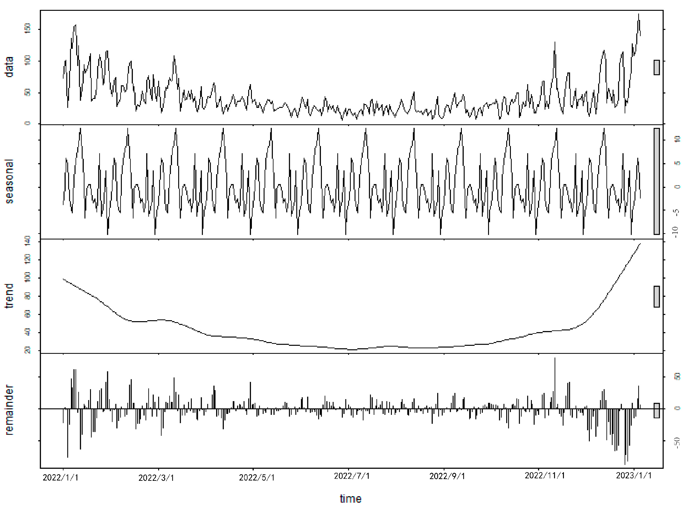
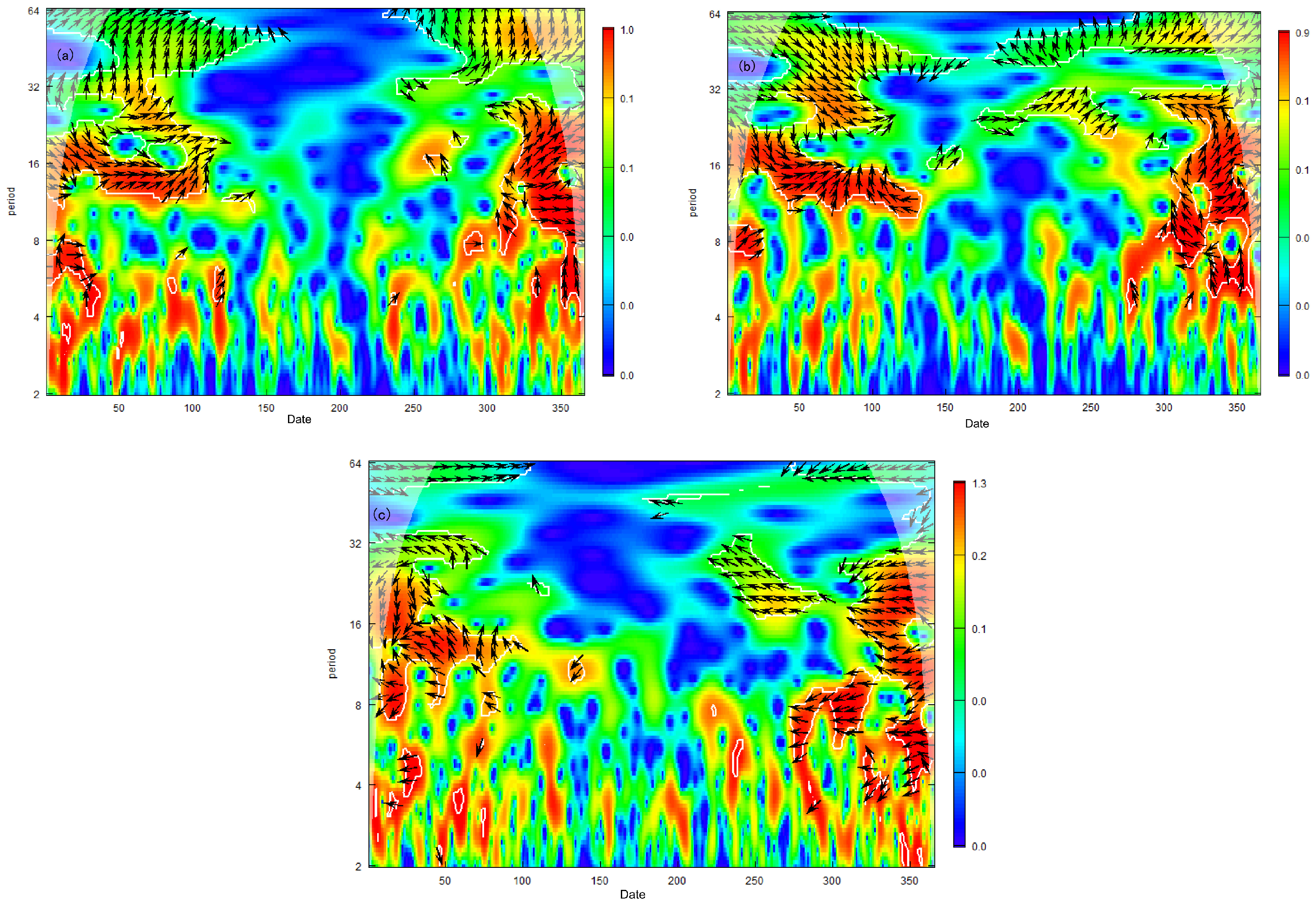
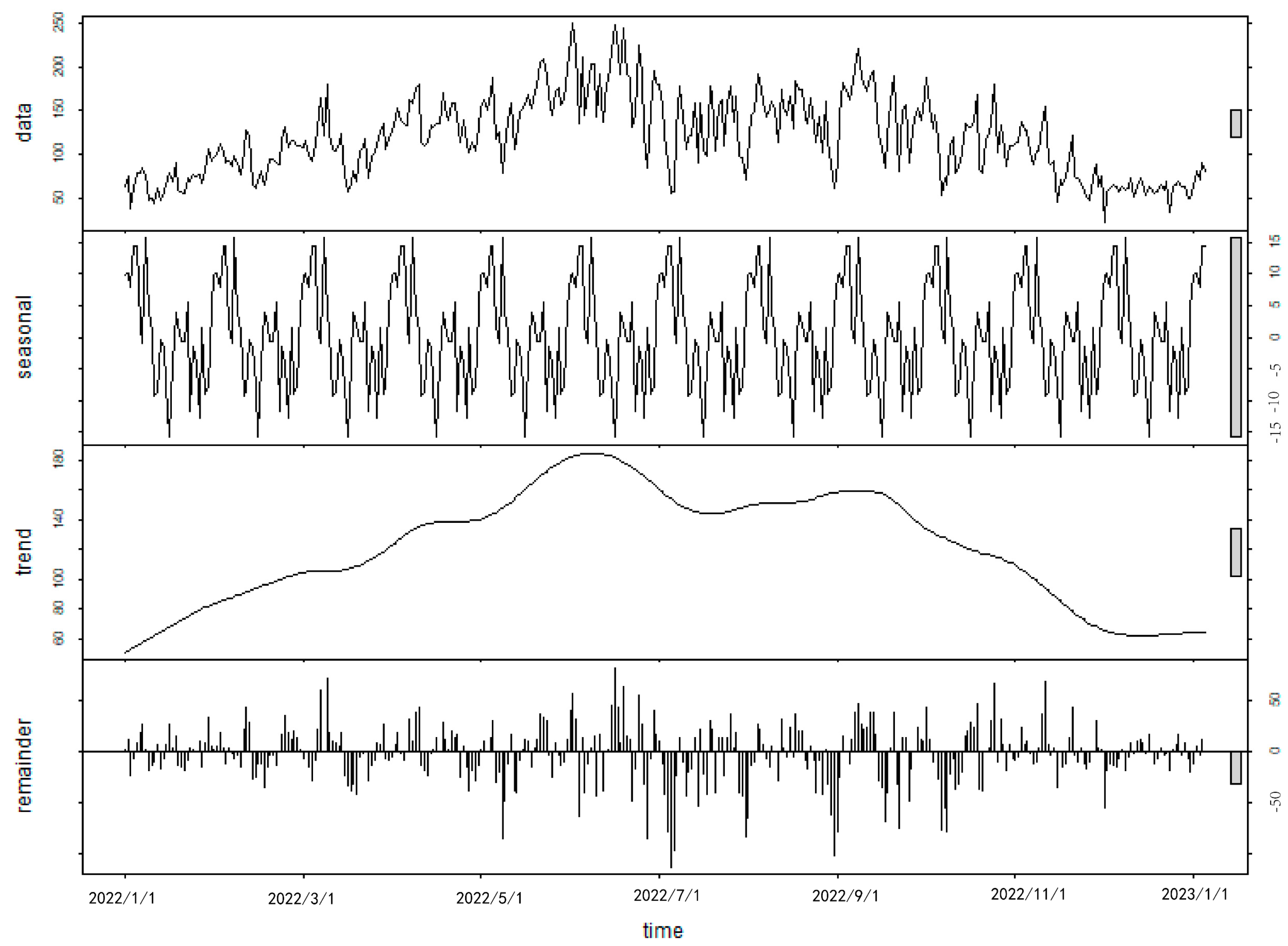
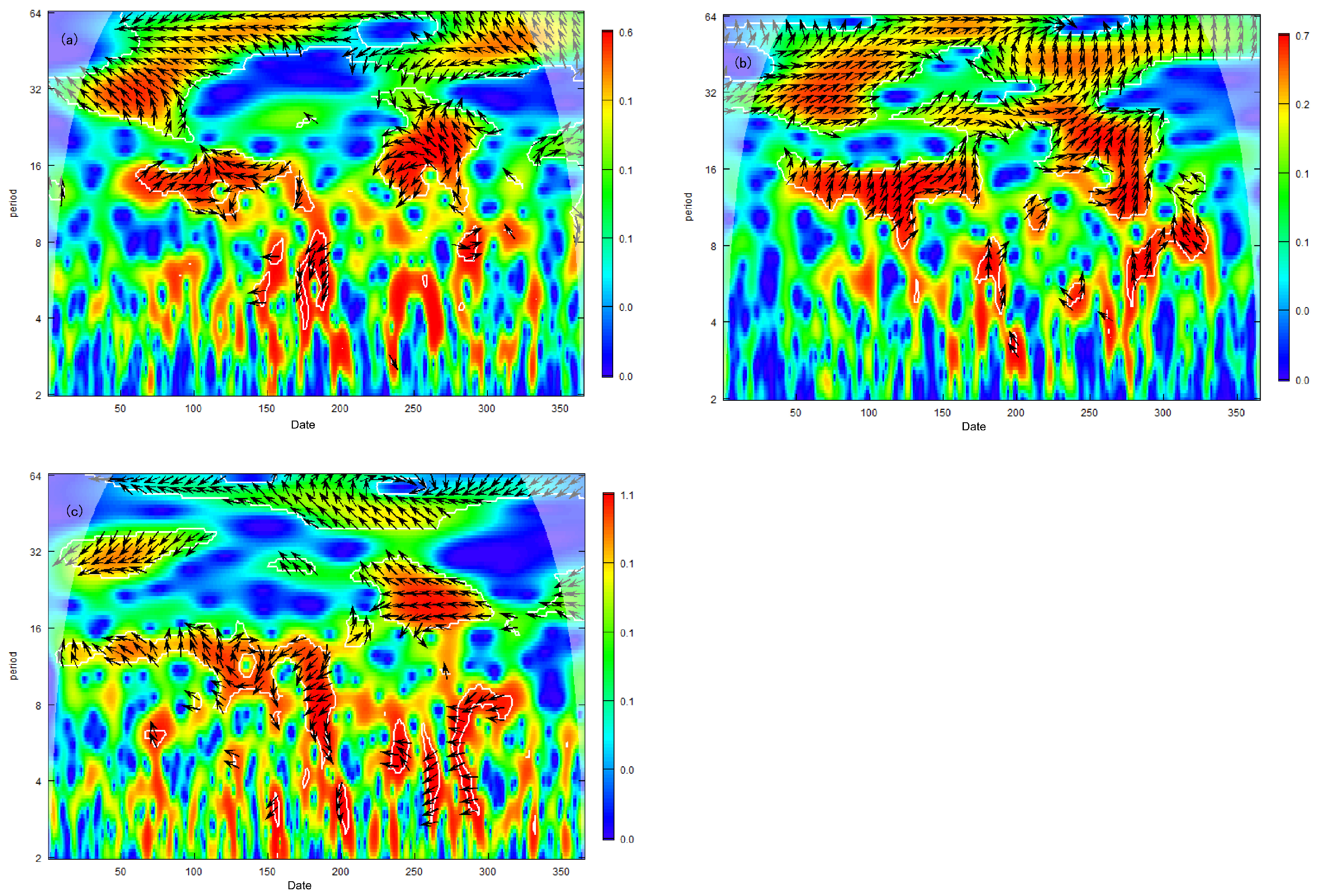
3.2.2. The Results of Time-Series Decomposition and Wavelet Transform

Time-series decomposition is a statistical method that breaks down time-series data into several basic components in order to better understand its intrinsic structure, trends, and periodicity. It is assumed that the time series of a given air pollutant is additive, consisting of long-term trends and seasonal and irregular short-term variables. Wavelet transform has the unique advantage of analyzing the correlation between atmospheric pollutant concentration and meteorological factors. It can simultaneously reveal the correlation features of the two on different time scales. Firstly, the wavelet coherence between pollutants and meteorological factors is calculated. It is a powerful tool for studying the correlation between two time series. The intensity of the correlation between pollutants and meteorological factors was explored through the coherence coefficient. The correlation between the two was explored from different time scales (short term/seasonal/long term). At the same time, this method can also be used to characterize the time change in correlation. The second step is to calculate the wavelet phase difference. The wavelet phase difference can be used to determine the corresponding time of pollutants to meteorological conditions and their lead–lag relationship.

Figure 9 shows the decomposition results of the periodic trend of PM_2.5 concentration in Zaozhuang City in 2022, that is, the original PM_2.5 concentration data are decomposed into seasonal components, trend components, and residual components. As shown in Figure 9, the original observation data show that the PM_2.5 concentration presents obvious fluctuation characteristics. PM_2.5 concentrations are generally in the range of 30–120 µg/m³. There are significant peaks around January and December, and lower levels around July. Seasonal trends show a steady cyclical pattern. Mainly due to the increase in heating emissions and unfavorable diffusion conditions, the peak occurred in winter (November–January). The summer trough (June–August) benefits from increased precipitation and improved atmospheric diffusion conditions. The spring and autumn transitional period shows moderate concentration levels. This annual cyclical fluctuation of about 50–60 µg/m³ is a significant feature of PM_2.5 variation. The trend item reveals the long-term direction of change throughout 2022. From January to March, there was a slow downward trend, which may reflect the reduction in emissions during the Spring Festival holiday. It remained relatively stable from April to September. It rose again in October, coinciding with the start of the heating season. The overall trend line indicates that the average annual PM_2.5 concentration in 2022 May improves slightly compared to previous years. The remainder term captures several unusual fluctuations: positive residual spikes in March and October, which may correspond to dust or straw-burning events.

Figure 10a shows a wavelet coherence map of PM_2.5 and relative humidity in Zaozhuang City, revealing the complex coupling relationship between the two on different time scales. From the short period (2–8 days), there is a significant coherence region (coherence coefficient > 0.8) in winter and autumn, which shows the in-phase change. This indicates that, when the relative humidity increases rapidly, the PM_2.5 concentration rises synchronously on the scale in the range of 2–8 days. This reflects the typical characteristics of high humidity promoting aerosol hygroscopic growth and secondary transformation under static and stable weather conditions in Zaozhuang City. From the perspective of the seasonal scale (16–32 days), a unique “coherent hole” appeared in spring, indicating that the humidity change from March to May had a weak effect on PM_2.5, which may be related to the frequent cold-air activities in Zaozhuang City in spring disrupting the local pollution accumulation process. In summer, it shows intermittent inverse-phase coherence, which reflects the dual effects of high humidity and PM_2.5 wet deposition. From the long-term trend (>32 days), it can be seen that the coherence of the year presents a “double-peak” structure. The first peak occurred in January–February, and the second, weaker peak occurred in October–November. It is worth noting that the coherence is generally weak from June to August.

Figure 10b shows the wavelet coherence map of PM_2.5 and temperature in Zaozhuang City. From the short period (2–8 days), it can be seen that the winter period presents a significant signal of strong coherence (coherence coefficient > 0.9), and the phase relationship shows that the decrease in temperature occurs simultaneously with the increase in PM_2.5 concentration. This reflects the dual role of the formation of the inversion layer and the increase in heating emissions during the transit of cold air in Zaozhuang City, especially in December. On the seasonal scale (16–32 days), a unique “coherent oscillation” pattern appears in spring, which is characterized by alternating changes in positive coherence in March–April and the negative interphase in April–May. This characteristic may be related to the frequent alternations in cold and warm air in spring in Zaozhuang City, which leads to the periodic change in pollutant diffusion conditions. From the long-term trend (>32 days), the year-round coherence showed significant seasonal differences, with winter and autumn maintaining a consistently high coherence values, while summer coherence significantly weakened.

Figure 10c shows the wavelet coherence diagram of PM_2.5 and wind speed in Zaozhuang City. A significant negative coherence band (coherence coefficient > 0.7) persists throughout the year. The phase arrows are consistent, indicating that there is an immediate response relationship between the increase in wind speed and the decrease in PM_2.5. The darkest coherent region is present in winter and autumn, indicating that, when the wind speed is lower than 2.5 m/s, it is easy to lead to a rapid accumulation of pollutants. In mid-April, there was a strong coherence period for 10 consecutive days, corresponding to the typical sand and dust transport process, and the increase in wind speed produced a special positive correlation with the temporary rise in PM_2.5. It is worth noting that the coherence range at the beginning of the heating season extended to a longer period, suggesting that the duration of static and stable weather was extended.

Figure 11 shows the time-series decomposition diagram of O₃ concentration, which clearly shows the seasonal component, trend component, and residual component of ozone variation. Seasonal components show strong cyclical patterns. O₃ concentrations peak in summer. The main reason is the strong sunshine and high-temperature conditions in summer, which accelerate the photochemical reaction of VOCs and NOx. O₃ concentrations reach a low point in winter, mainly due to reduced solar radiation and lower temperatures. Spring and autumn show a rapid rise and fall transition. The trend component reveals two important features. From April to September, the ozone showed a slow, rising trend. The overall trend line was stable throughout the year, indicating that short-term governance measures had a limited influence on O₃. Remainder captures several important exceptions. Positive residual spikes occurred in May and July, which may correspond to extreme hot weather or transmission pollution events.

Figure 12a shows the wavelet coherence between O₃ and relative humidity in Zaozhuang City. Intermittent positive coherence patches appear in spring and early autumn, indicating that moderate humidity (50–60%) is favorable for the secondary transformation of O₃ precursors under certain weather conditions. A “two-valley” coherent structure is observed throughout the year, and the first low coherence valley appears in January–March, when low-temperature conditions dominate the background concentration of O₃. The second valley value occurs in July–August, showing the extremely frequent wet weather that weakens the correlation between humidity and O₃.

Figure 12b shows the wavelet coherence between O₃ and temperature in Zaozhuang City. Strong positive coherence (coherence coefficient > 0.8) appears in summer. The phase arrows consistently point horizontally to the right, indicating that every 1 °C increase in temperature causes an 8–12 µg/m³ increase in O₃ concentrations over a 3-day period. Especially in the high-temperature season, from July to August, the coherent band presents a deep-red continuous distribution, showing that the temperature is the decisive control factor of the photochemical reaction rate.

Figure 12c shows the wavelet coherence between O₃ and wind speed in Zaozhuang City. During the medium period (16–32 days), multiple red and yellow regions appear in the figure, indicating that the coherence of O₃ concentration and wind speed is high in this period range, and there may be a strong interaction. However, the correlation is weak in short and long periods.

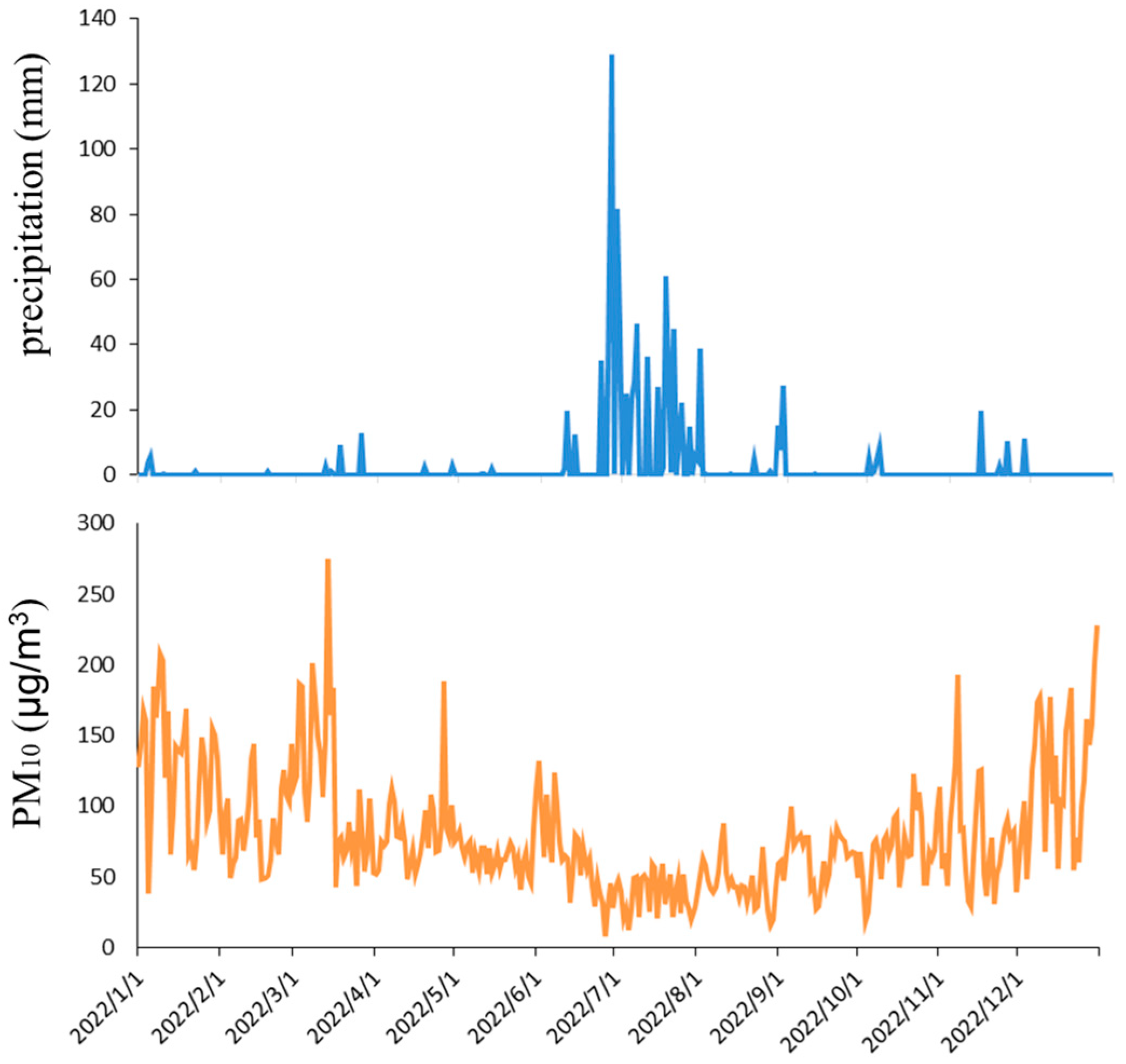
3.2.3. Correlation Between PM₁₀ and Precipitation

Relevant studies show that precipitation is an important factor affecting pollutant concentration when pollution sources are relatively stable. In the event of rainfall, raindrop adsorption and rain erosion under clouds have the most direct influence on the concentration of atmospheric pollutants, especially particulate matter [32,33,34]. In particular, rain erosion under clouds can effectively reduce the concentration of atmospheric pollutants [35,36]. The degree of improvement in air quality during precipitation is also related to the amount of precipitation and the atmospheric pollution before precipitation [37]. Therefore, this study explored the relationship between precipitation and PM₁₀ in Zaozhuang City.

The distribution of atmospheric pollutant PM₁₀ and precipitation in Zaozhuang City in 2022 is shown in Figure 13. As can be seen from Figure 13, the decrease in PM₁₀ is mostly accompanied by precipitation, and precipitation is proportional to the decrease in PM₁₀, that is, the greater the precipitation, the greater the decrease in PM₁₀, and the PM₁₀ concentration will rise rapidly at the end of the precipitation process.

In order to more accurately analyze the impact of precipitation on pollutants, the PM₁₀ value before and after the daily precipitation reaches 10 mm is selected for statistical analysis, and the results are shown in

Table 7. Comparison of PM₁₀ concentration before and after a precipitation level of more than 10 mm in Zaozhuang City in 2022.

Date	Precipitation/mm	PM10 of the Day (µg/m3)	PM10 of the Previous Day (µg/m3)	Rate of Change (%)
25 March 2022	12.9	44	82	53.6
9 June–10 June 2022	21.6	74	124	59.7
23 June 2022	35	29	44	65.9
26 June–30 June 2022	128.9	8	62	12.9
10 July 2022	36.5	13	32	40.6
28 August–30 August 2022	49.6	16	71	22.5
22 November–23 November 2022	10.5	31	78	39.7

. It can be seen from the table that precipitation has an obvious clearing effect on PM₁₀.

4. Conclusions and Prospect

4.1. Conclusions

(1)

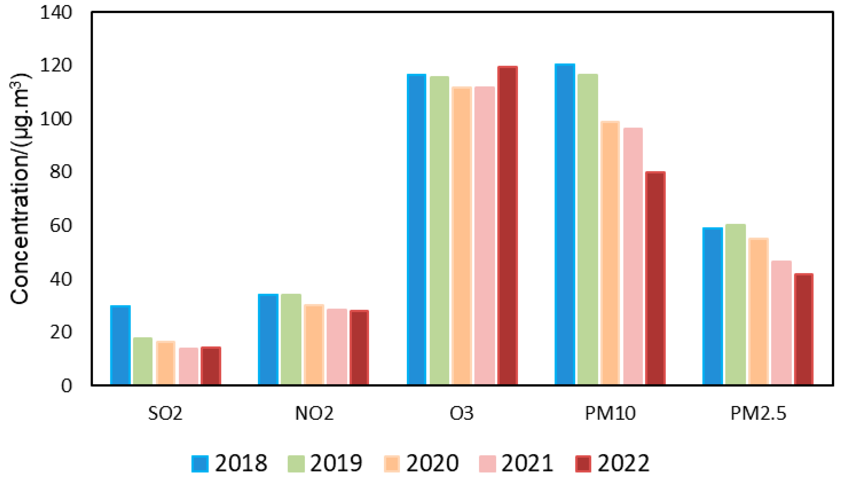
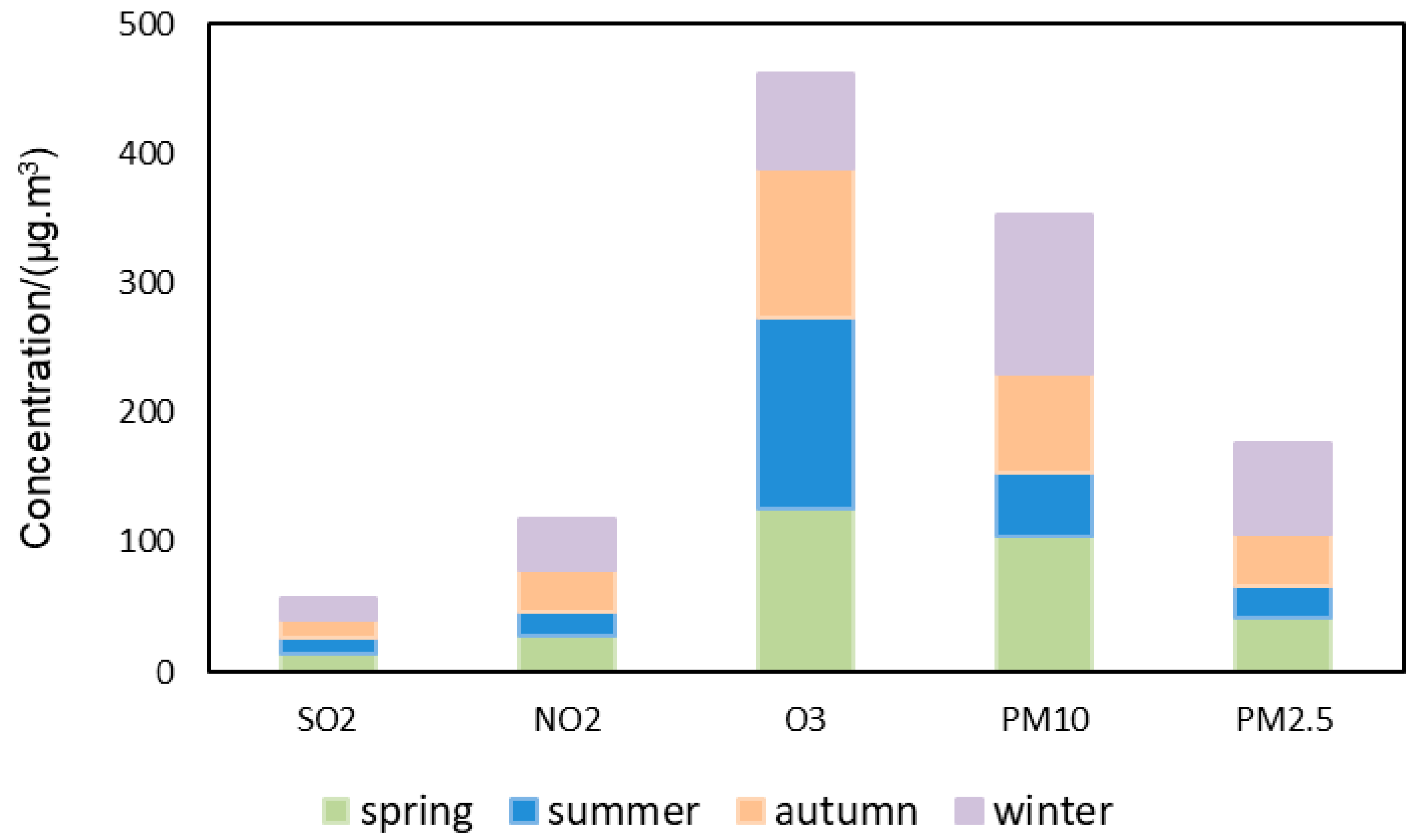
The concentration of air pollutants in Zaozhuang City generally showed a decreasing trend from 2018 to 2022. NO₂, SO₂, PM_2.5, and PM₁₀ concentrations decreased by 17.3%, 52.2%, 28.9%, and 33.6%, respectively, in 2022 compared with 2018, while the concentration of O₃ in 2022 was 2.5% higher than that in 2018. From the perspective of seasonal variation, the concentrations of SO₂, PM_2.5, PM₁₀, CO, and NO₂ were the highest in winter and the lowest in summer. The O₃ concentration is distributed from high to low in summer, spring, autumn, and winter.

(2)

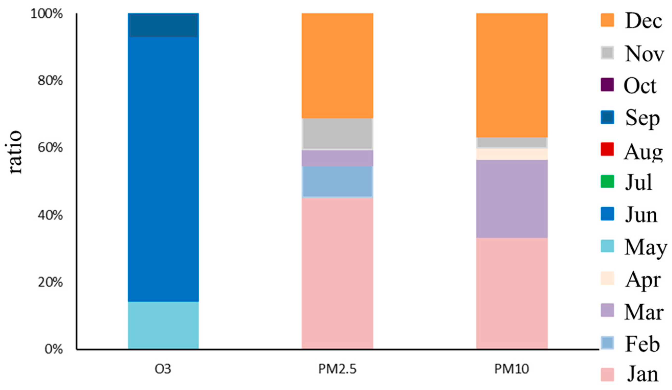
The monthly changes in SO₂, CO, NO₂, PM_2.5, and PM₁₀ were U-shaped. High values were concentrated in December and January, while low values were concentrated in June, July, August, and September. The monthly variation in O₃ showed a bimodal variation. It peaked in June and September. The maximum daily average concentrations of CO, NO₂, SO₂, PM_2.5, and PM₁₀ all appeared on Monday, and the daily average concentration was basically higher on weekdays than on weekends.

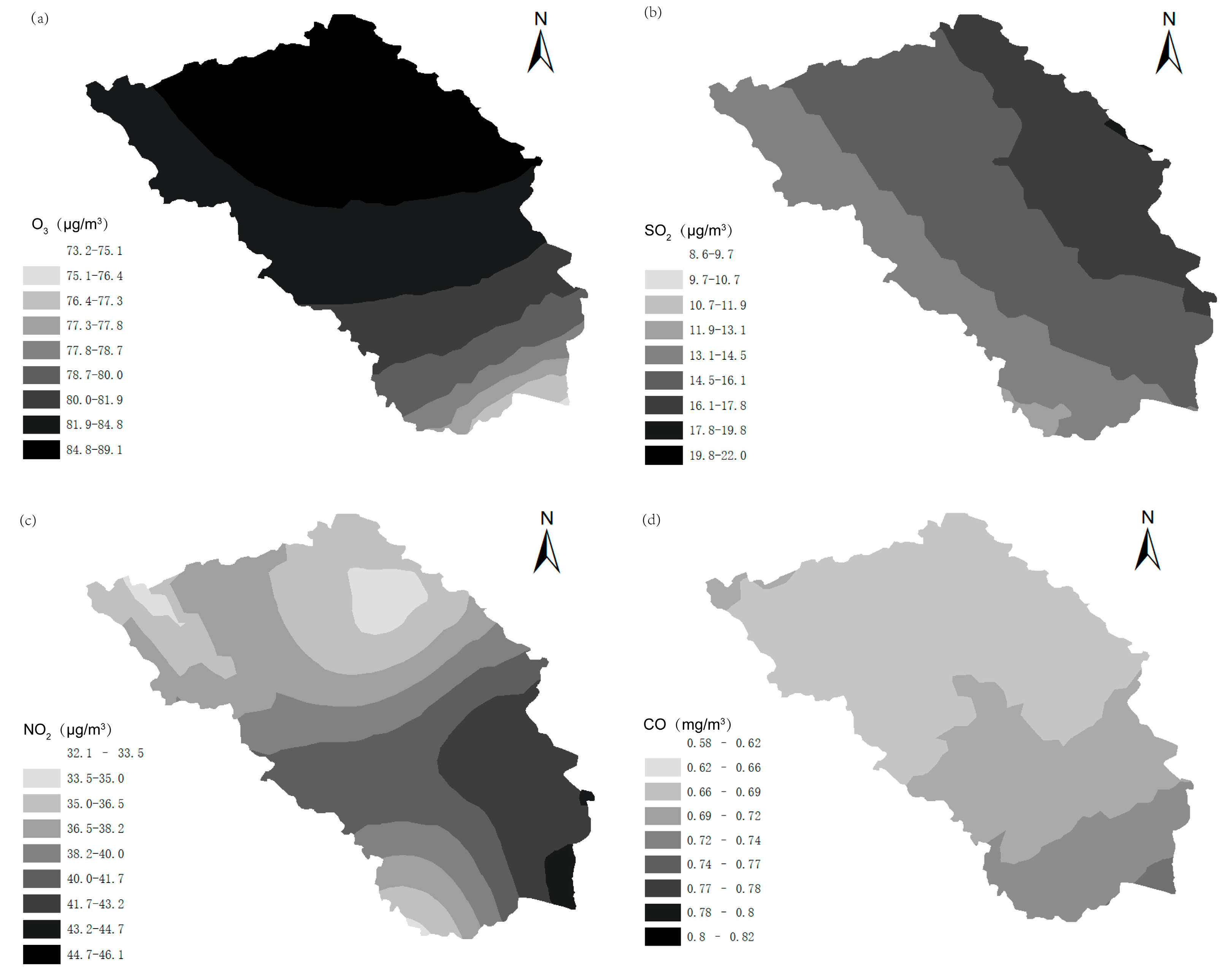
(3)

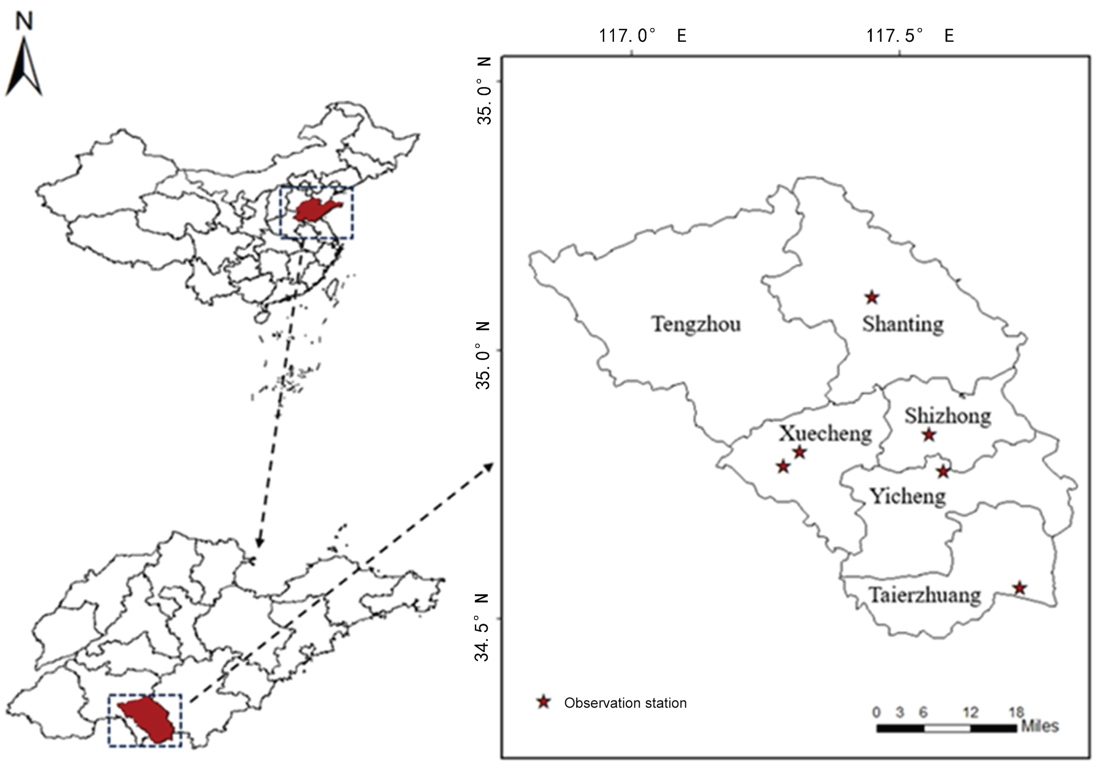
The spatial distribution characteristics of NO₂, CO, PM_2.5, and PM₁₀ were basically the same, that is, they gradually decreased from the south to the north, and the lowest values mostly appeared in the Shanting area. The high O₃ and SO₂ values were distributed in the economically developed and industrialized Shizhong District, Xuecheng District, and Tengzhou City.

(4)

All the pollutants were almost negatively correlated with the wind speed. The main reason is that, when the wind speed is high, it is conducive to the diffusion of pollutants.

4.2. Recommendations

(1)

Enhanced monitoring density and prediction accuracy

Real-time monitoring data of pollutant concentration and long-term and short-term concentration predictions are important bases to guide our planning and deployment. Therefore, it is very important to improve the monitoring accuracy and prediction accuracy. First of all, increase the monitoring stations as much as possible and make a reasonable distribution. At present, the monitoring stations in Shandong Province are relatively concentrated, and the state control stations in Jinan City are significantly greater than those in other cities. It is hoped that the monitoring of non-provincial cities will be strengthened. Secondly, more mobile monitoring vehicles can be used in appropriate areas to monitor the concentration distribution of pollutants in real time and accurately.

(2)

Strengthen early-warning publicity

Air pollutant warnings will be issued through multiple channels. The power of the Internet can be better utilized, combined with social media and short video platforms, to provide timely warnings during periods of high pollutant concentration, so that the public can be prepared for the situation. These should target June and September to strengthen the O₃ pollution early-warning publicity; January and December to strengthen PM_2.5 early-warning publicity; and January, March, and April to strengthen PM₁₀ early-warning publicity. Volunteers can be gathered to communicate with the community through the production of publicity banners, slogans, and other forms of warning, to publicize air pollutant-related knowledge to the community residents, so that more people consciously realize the significance of environmental protection and actively take environmental protection actions.

(3)

Call on enterprises to reduce emissions and strengthen supervision

O₃ and PM_2.5 are the main atmospheric pollutants in Zaozhuang City. Reducing VOCs and NOx, which are common precursors of O₃ and PM_2.5, is a basic measure to control secondary air pollutants. At present, there are many industries that emit VOCs and NO_X in Zaozhuang City, and the emissions are high. They have a significant impact on air quality in the region. Therefore, the government should strengthen supervision, implement regulatory policies, and urge enterprises with high emissions to rectify their behavior.

4.3. Prospect

This research has some limitations. The follow-up research work can be improved and overcome the following aspects.

The diffusion of air pollutants is a complicated process. If the chemical-change process of pollutants is considered in the analysis of air pollution diffusion, this error can be limited. The interpolation accuracy of the model can achieve better results. In the existing air-quality assessment system, only six kinds of pollutants are considered. With the improvement of people’s environmental-quality requirements and the intensification of environmental pollution, air-quality evaluations are no longer limited to the existing six pollutants, and new pollution elements will be added to the environmental-quality evaluation system. In addition, mitigation strategies or long-term impacts on health and the environment could be explored in future studies.

References

1. Wang, C.; Guo, J.; Liu, J. Green roofs and their effect on architectural design and urban ecology using deep learning approaches. Soft Comput. 2024, 28, 3667–3682. [Google Scholar] [CrossRef]
2. Yan, J.; Geng, J.; Su, F. Estimation of the Ecosystem Service Value of the Yellow River Delta-Laizhou Bay Coastal Zone Considering Regional Differences and Social Development. Environ. Manag. 2024, 74, 192–205. [Google Scholar] [CrossRef] [PubMed]
3. Bin, X.; Zhong, Y.; Bin, J.L. Research on the control of overburden deformation by filling ratio of cementing filling method with continuous mining and continuous backfilling. Environ. Sci. Pollut. Res. 2023, 30, 26764–26777. [Google Scholar] [CrossRef]
4. Shen, F.; Song, L.; Min, J.; He, Z.; Shu, A.; Xu, D.; Chen, J. Impact of assimilating pseudo-observations derived from the “Z-RH” relation on analyses and forecasts of a strong convection case. Adv. Atmos. Sci. 2025, 42, 1010–1025. [Google Scholar] [CrossRef]
5. Shu, A.; Shen, F.; Li, H.; Min, J.; Luo, J.; Xu, D. Impacts of assimilating polarimetric radar KDP observations with an ensemble Kalman filter on analyses and predictions of a rainstorm associated with Typhoon Hato (2017). Q. J. R. Meteorol. Soc. 2025, 17, e4943. [Google Scholar] [CrossRef]
6. Zheng, Y.; Kolditz, O.; Ma, K.Y. Environmental earth sciences: Advancing geosphereplus knowledge for environmental problem solving. Environ. Earth Sci. 2023, 82, 445. [Google Scholar] [CrossRef]
7. Guo, Q.; Wang, Y.; Zhang, Y.; Yi, M.; Zhang, T. Environmental migration effects of air pollution: Micro-level evidence from China. Environ. Pollut. 2022, 292 Pt A, 118263. [Google Scholar] [CrossRef]
8. Zhang, J.; Luo, L.; Chen, G.; Ai, B.; Wu, G.; Gao, Y.; Lip, G.; Lin, H.; Chen, Y. Associations of ambient air pollution with incidence and dynamic progression of atrial fibrillation. Sci. Total Environ. 2024, 951, 175710. [Google Scholar] [CrossRef]
9. Kara, Y.; Evik, S.E.Y.; Toros, H. Comprehensive analysis of air pollution and the influence of meteorological factors: A case study of Adiyaman province. Environ. Monit. Assess. 2024, 196, 525. [Google Scholar] [CrossRef]
10. Maltby, T.; Birch, S.; Fagan, A.; Subai, M. What is the role of activism in air pollution politics? understanding policy change in Poland. Environ. Plan. C Politics Space 2024, 42, 1332–1351. [Google Scholar] [CrossRef]
11. Shen, L.; Yang, Z.; Du, X.; Wei, X.; Chen, X. A health risk-based threshold method to evaluate urban atmospheric environment carrying capacity in Beijing-Tianjin-Hebei (bth) region. Environ. Impact Assess. Rev. 2022, 92, 106692. [Google Scholar] [CrossRef]
12. Liu, P.; Shao, L.; Li, Y.; Jones, T.; Cao, Y.; Yang, C.X.; Zhang, M.; Santosh, M.; Feng, X.; Bérubé, K. Microplastic atmospheric dustfall pollution in urban environment: Evidence from the types, distribution, and probable sources in Beijing, China. Sci. Total Environ. 2022, 838, 155989. [Google Scholar] [CrossRef] [PubMed]
13. Guo, J.; Li, Z.; Zhang, B. Interaction patterns between economic growth and atmospheric environment in China under the “carbon neutrality” target. Environ. Sci. Pollut. Res. 2023, 30, 98231–98245. [Google Scholar] [CrossRef] [PubMed]
14. Zhu, D.; Liang, G. Atmospheric pollution status quo and prevention proposals in Zaozhuang city. J. Environ. Manag. Coll. China 2014, 24, 18–20+45. [Google Scholar] [CrossRef]
15. Liu, Y.; Wang, M.; Gui, C. Spatial and temporal distribution characteristics and correlation analysis of PM2.5 in urban agglomeration of China’s industrial base. Sci. Technol. Eng. 2018, 18, 184–189. [Google Scholar] [CrossRef]
16. Ma, M.; Yang, X.; Ding, F. Spatial and temporal distribution of air pollutants in northern and southern China. Environ. Sci. Technol. 2018, 41, 187–197. [Google Scholar] [CrossRef]
17. Chen, S.; Wang, C.; Xie, T. Distribution characteristics of atmospheric particulate matter in cold and warm seasons in mainland China in 2014. J. Lanzhou Univ. 2018, 54, 167–174+183. [Google Scholar] [CrossRef]
18. Zang, X.; Lu, G.; Yao, H. Research on the spatiotemporal distribution characteristics of major atmospheric pollutants in China. J. Ecol. Environ. 2015, 24, 1322–1329. [Google Scholar] [CrossRef]
19. Li, X.; Abdullah, L.; Sobri, S.; Said, M.; Hussain, S.; Tan, P.; Hu, J. Long-term air pollution characteristics and multi-scale meteorological factor variability analysis of mega-mountain cities in the Chengdu-Chongqing economic circle. Water Air Soil Pollut. 2023, 234, 328. [Google Scholar] [CrossRef]
20. Zhang, L.; Xu, X.; Zhang, Y.; Zhang, X.; Wu, J.; Sheng, X.; Chen, F.; Chen, L.; Ge, X.; Wu, H. Characteristics of air pollution complex in a typical chemical industrial development zone in eastern China. Atmos. Environ. 2024, 319, 120274. [Google Scholar] [CrossRef]
21. Li, J. Structural characteristics and evolution trend of collaborative governance of air pollution in “2 + 26” cities from the perspective of social network analysis. Sustainability 2023, 15, 5943. [Google Scholar] [CrossRef]
22. Guan, J.; Geng, Z.; Yang, F.; Zhang, X.; Chen, S.; Guo, Y. Analysis on temporal variation law of ozone pollution and meteorological driving factors in pudong new area of Shanghai. Environ. Prog. Sustain. Energy 2023, 42, e14089. [Google Scholar] [CrossRef]
23. Wang, J.; Zhao, Y.; Xu, M. Distribution characteristics of six criteria air pollutants under different air quality levels in Cangzhou city, China. J. Health Environ. Res. 2022, 8, 9–15. [Google Scholar] [CrossRef]
24. Matheron, G. Principles of geostatistics. Econ. Geol. 1963, 58, 1246–1266. [Google Scholar] [CrossRef]
25. Hock, R.; Jensen, H. Application of kriging interpolation for glacier mass balance computations. Geogr. Ann. Ser. A Phys. Geogr. 1999, 81, 611–619. [Google Scholar] [CrossRef]
26. Zhang, S.; Wan, Z.; Wang, X.; Xu, A.; Chen, Z. Analysis of Flight Loads during Symmetric Aircraft Maneuvers Based on the Gradient-Enhanced Kriging Model. Aerospace 2024, 11, 334. [Google Scholar] [CrossRef]
27. Gocic, M.; Trajkovic, S. Analysis of changes in meteorological variables using Mann-Kendall and Sen’s slope estimator statistical tests in Serbia. Glob. Planet. Change 2013, 100, 172–182. [Google Scholar] [CrossRef]
28. Zhang, X.; Xu, D.; Shen, F.; Min, J. Impacts of offline nonlinear bias correction schemes using the machine learning technology on the all-sky assimilation of cloud-affected infrared radiances. J. Adv. Model. Earth Syst. 2024, 16, e2024MS004281. [Google Scholar] [CrossRef]
29. Zhang, X.; Xu, D.; Min, J.; Li, H.; Shen, F.; Lei, Y. A Machine Learning-based Bias Correction Scheme for the All-Sky Assimilation of AGRI Infrared Radiances in a Regional OSSE Framework. IEEE Trans. Geosci. Remote Sens. 2024, 62, 5407314. [Google Scholar] [CrossRef]
30. Kamińska, J. The use of random forests in modelling short-term air pollution effects based on traffic and meteorological conditions: A case study in Wrocaw. J. Environ. Manag. 2018, 217, 164–174. [Google Scholar] [CrossRef]
31. Kamińska, J.; Turek, T. Explicit and implicit description of the factors impact on the NO2 concentration in the traffic corridor. J. Environ. Sci. Eng. 2023, 12, 456–478. [Google Scholar] [CrossRef]
32. Bai, Y.; Qi, H.; Zhao, T.; Yang, H.; Liu, L.; Cui, C. Analysis of meteorological conditions and diurnal variation characteristics of PM2.5 heavy pollution episodes in the winter of 2015 in Hubei province. Acta Meteorol. Sin. 2018, 76, 803–815. [Google Scholar] [CrossRef]
33. Zhou, H.; Li, X.; Liu, Y.; Tian, X.; Wen, J. Wet Scavenging Effect of Precipitation on PM2.5 Concentration in Langfang of Hebei Province. Environ. Prot. Sci. 2020, 46, 70–75. [Google Scholar] [CrossRef]
34. Yu, C.; Deng, X. The scavenging effect of precipitation and wind on PM2.5 and PM10. J. Environ. Sci. 2018, 38, 4620–4629. [Google Scholar] [CrossRef]
35. Zhang, D. Study on Reducing Effect of Artificial Precipitation on Concentration of Atmospheric Particulate Pollutants. Environ. Sci. Manag. 2021, 46, 43–47. [Google Scholar] [CrossRef]
36. Liao, D.; Xiang, B.; Liu, Y. Study on the Correlation Between Meteorological Elements and Air Quality in Chongqing. Environ. Impact Assess. 2020, 42, 75–80. [Google Scholar] [CrossRef]
37. Luan, T.; Guo, X.; Zhang, T.; Guo, L. The scavenging process and physical removing mechanism of pollutant aerosols by different precipitation intensities. J. Appl. Meteorol. Sci. 2019, 30, 279–291. [Google Scholar] [CrossRef]
Figure 1. Location map of the Zaozhuang environmental monitoring station.
Atmosphere 16 00493 g001
Figure 2. The proportion of pollutants exceeding the standard in Zaozhuang City by month in 2022.
Atmosphere 16 00493 g002
Figure 3. Annual changes in pollutants from 2018 to 2022.
Atmosphere 16 00493 g003
Figure 4. Seasonal changes in pollutants from 2018 to 2022.
Atmosphere 16 00493 g004
Figure 5. Monthly changes in pollutants in Zaozhuang from 2018 to 2022.
Atmosphere 16 00493 g005
Figure 6. Changes in pollutants on weekdays and weekends in 2022.
Atmosphere 16 00493 g006
Figure 7. Spatial distribution of O3 (a); SO2 (b); NO2 (c); CO (d); PM2.5 (e); PM10 (f) in Zaozhuang City in 2022.
Atmosphere 16 00493 g007aAtmosphere 16 00493 g007b
Figure 8. The analysis result based on DBSCAN.
Atmosphere 16 00493 g008
Figure 9. Time-series decomposition of PM2.5 concentration in 2022.
Atmosphere 16 00493 g009
Figure 10. Wavelet coherence spectra of PM2.5 with relative humidity (a), temperature (b), and wind speed (c). (The direction of the arrow indicates the phase difference between two signals, that is, the leading or lagging relationship in time. An arrow pointing to the right indicates that the two signals are in phase, that is, they change synchronously on this time scale. The arrow to the left indicates that the two signals are in opposite phases, that is, their changing trends are opposite. An upward arrow indicates that PM2.5 lags behind meteorological elements. The downward arrow indicates that the change of PM2.5 occurs earlier than that of meteorological elements. The area surrounded by white contour lines indicates that the coherence has passed the significance test (p < 0.05). That is, the coherence result within the white line is statistically significant).
Atmosphere 16 00493 g010
Figure 11. Time-series decomposition of O3 concentration in 2022.
Atmosphere 16 00493 g011
Figure 12. Wavelet coherence spectra of O3 with relative humidity (a), temperature (b), and wind speed (c). (The direction of the arrow indicates the phase difference between two signals, that is, the leading or lagging relationship in time. An arrow pointing to the right indicates that the two signals are in phase, that is, they change synchronously on this time scale. The arrow to the left indicates that the two signals are in opposite phases, that is, their changing trends are opposite. An upward arrow indicates that O3 lags behind meteorological elements. The downward arrow indicates that the change of O3 occurs earlier than that of meteorological elements. The area surrounded by white contour lines indicates that the coherence has passed the significance test (p < 0.05). That is, the coherence result within the white line is statistically significant).
Atmosphere 16 00493 g012
Figure 13. Time series of PM10 and precipitation in Zaozhuang City in 2022.
Atmosphere 16 00493 g013