Ionospheric Anomaly Identification: Based on GNSS-TEC Data Fusion Supported by Three-Dimensional Spherical Voxel Visualization

Abstract

Ionospheric tomography, an effective method for reconstructing 3-D electron density, is traditionally pictured by 3-D IED (ionospheric electron density) slices to express ionospheric disturbances, which may overlook the critical information in 3-D spherical manifold space. Here, we develop a novel visualization framework that integrates tomography reconstruction with a spherical latitude–longitude grid system, enabling the comprehensive characterization of 3-D IED dynamic evolution in 3-D manifold spherical space. Through this method, we visualized two cases: the Hualien earthquake on 2 April 2024 and the geomagnetic storm on 24 April 2023. The results demonstrate the evolution of the electron density during earthquake and geomagnetic storms in the real 3-D space, showing that seismic events induce bottom-up IED negative anomalies localized near epicenters, while geomagnetic storms trigger top-down depletion processes, with IED propagating from higher altitudes in the real 3-D manifold space. Compared to the conventional slice, our visualization model can visualize the characteristics, with the coverage area being observed to increase with the altitude within the same geospatial coordinates. This framework can advance the identification of ionosphere anomalies by enabling the precise differentiation of anomaly sources. This work bridges gaps in geospatial modeling by harmonizing ionospheric tomography with Earth system grids, offering a feasible solution for analyzing multi-scale ionospheric phenomena.

1. Introduction

The ionosphere is a 3-D shell-like manifold region located 60 to 1000 km above the Earth’s surface, containing a significant number of free electrons and ions [1,2]. Variations in the distribution of ions and electrons within the ionosphere result in a multi-layered structure, with primary activity concentrated in the F layer [3]. Activities within the Earth’s atmosphere, such as large-scale disasters (earthquakes, volcanic eruptions, etc.), as well as cosmic events like magnetic storms impact the electron density within the ionospheric structure, leading to changes in the electron density throughout this 3-D shell [4,5,6]. Therefore, monitoring the 3-D spatiotemporal dynamic changes that occur in the ionosphere is significant for providing early warnings of disasters.

Ionospheric tomography is an effective method for exploring 3-D variations in electron density, utilizing GNSS technology to reconstruct 3-D images of the IED (ionospheric electron density) [7,8,9]. This technique analyzes the signal delays experienced by GNSS signals as they propagate through the ionosphere [10]. Based on different basis functions, the tomographic models are primarily categorized into function-based and voxel-based models [11]. Function-based models simulate and express the spatial distribution of the IED using a set of functions; however, it is often challenging to identify suitable parameters in practical applications [12]. In contrast, voxel-based models typically discretize the ionosphere into numerous voxels using 3-D grids, each defined by latitude, longitude, and altitude, and assume homogeneity within each voxel [13]. This approach has been widely applied in the field of ionospheric anomaly monitoring. For instance, He [6] employs 3-D tomography to investigate the pre-seismic anomalies associated with the 2015 Illapel earthquake with a voxel grid of $1.5°\times 1.2°\times 100\mathrm{k}\mathrm{m}$. He demonstrates variations in the electron density at different altitudes, times, and locations using slices, revealing that negative electron density anomalies appear above positive anomalies prior to the earthquake. Similarly, Cahyadi [14] utilizes voxel-based 3-D tomography to reveal an amplitude of 0.4 TECU approximately 10–15 min after the 2018 Palu earthquake with a grid of $1°\times 1°\times 75\mathrm{k}\mathrm{m}$. In addition to ionospheric anomalies induced by terrestrial activities, anomalies caused by extraterrestrial events are also frequently analyzed using voxel-based 3-D tomography. Prol [15] constructs a global tomography to analyze the 2015 Geomagnetic Storm with a grid of $2°\times 2°\times 20\mathrm{k}\mathrm{m}$, depicting a phenomenon of equatorial ionization anomaly enhancements and depletion. These studies have established varying voxel unit dimensions according to their specific requirements, yet all uniformly presume intrinsic homogeneity within individual voxels. This assumption frequently results in voxel variations and consequential inaccuracies in analytical outcomes. Recently, Chen [4] proposed a node parameterization tomography that assumes an inhomogeneous distribution of IED in the space. This novel framework theoretically enables the construction of tomographic models at arbitrary spatial scales. Regarding 3-D ionosphere representation, the prevailing methodologies predominantly rely on the vertical stacking of two-dimensional planar electron density slices or the analysis of latitudinal/longitudinal cross-sections. Such conventional practices may overlook critical information regarding the actual morphology of the ionosphere in its 3-D context.

In recent years, significant advances have been made in 3-D representations of the Earth system through spatial grid frameworks, notably advancing the visualization of 3-D electron density distributions. These frameworks, collectively termed ESSG (Earth System Spatial Grids) or DGGS (Discrete global grid system), employ discrete grid-based methodologies for encoding, analyzing, and visualizing the objects or phenomena on the earth [16,17]. ESSG are primarily categorized into spherical polyhedral models and latitude–longitude grid systems [18,19]. Spherical polyhedral models are constructed through the spherical projection of regular polyhedron edges, forming great circle arcs that generate global coverage through recursive subdivision [20,21,22]. While effective for managing multi-resolution spatial data sets, these models exhibit limitations in direct correlation with conventional latitude–altitude coordinate systems. Conversely, latitude–longitude grids partition space into volumetric units defined by longitudinal, latitudinal, and altitudinal dimensions, demonstrating superior compatibility with voxel-based tomographic modeling [23]. While most existing methods focus on the representation of 3-D spherical surfaces, the expression of 3-D spheroids has not been adequately addressed. Previous implementations by Wu and He have successfully demonstrated 3-D ionospheric electron density visualization using SDOG (spheroid degenerated octree grid) within the 3-D spheroids. However, their study predominantly emphasizes global-scale visualization patterns while lacking the analysis of local cases. In addition, the complex grid and structure also make it difficult to reproduce the visualization process [24,25].

Therefore, this study proposes a visualization modeling framework employing spherical latitude–longitude grid systems that can correspond well with the voxel grid. Furthermore, two case studies are conducted through this framework to visualize the ionospheric anomalies: the geomagnetic storm ionosphere anomaly on 20 April 2023, and the 2024 Hualien earthquake ionosphere anomaly.

2. Datasets and Methods

2.1. Materials

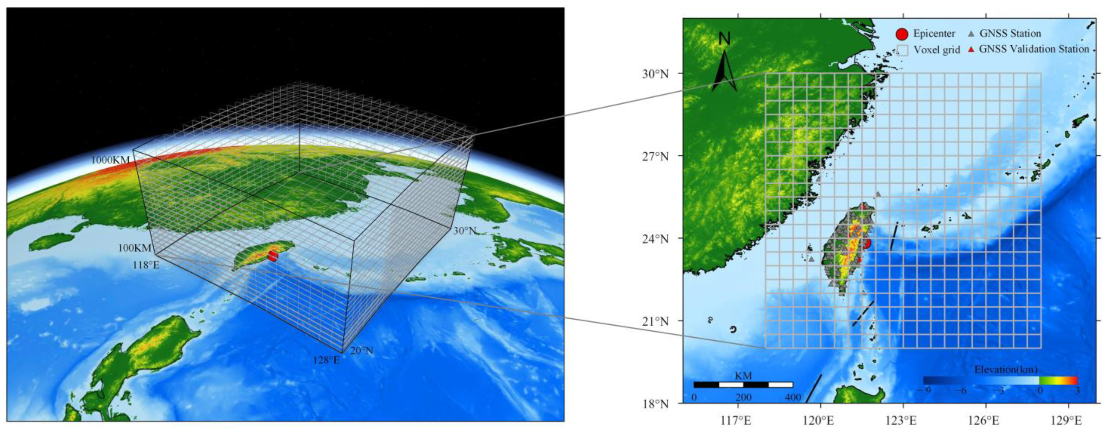
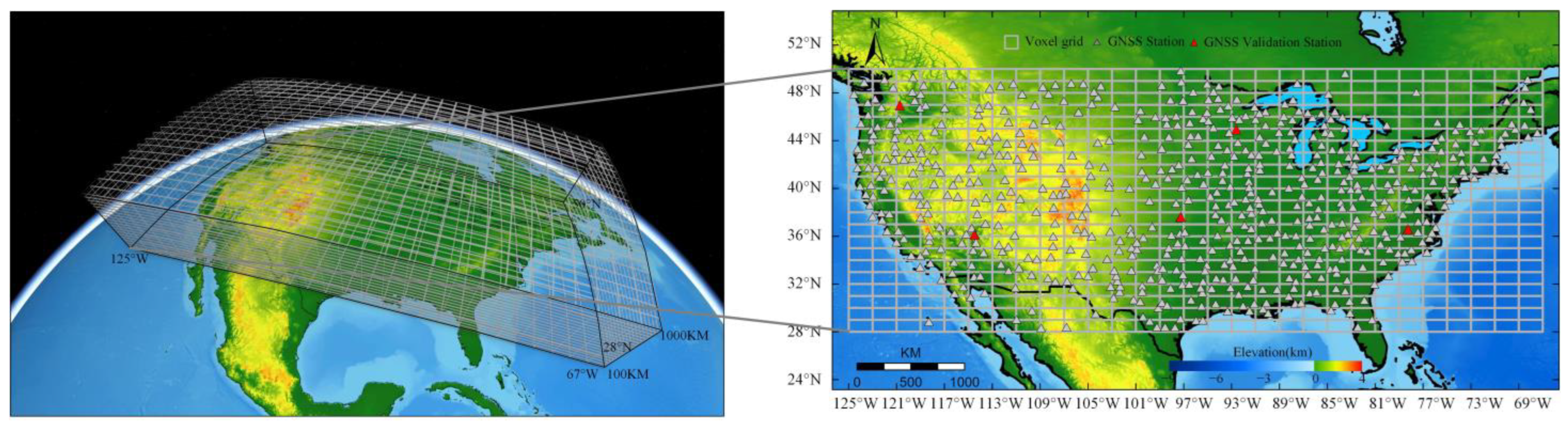
2.1.1. GNSS Data

To demonstrate the 3-D variation in ionosphere anomalies, this study selected two typical cases: the M7.4 Taiwan Earthquake that occurred within the Earth’s magnetosphere on 2 April 2024 and the outer space geomagnetic storm that occurred in the United States on 20 April 2023. As for earthquake, this study utilized GNSS data from the ground stations of the Taiwan Seismological and Geophysical Data Management System. To identify anomalies, 127 GNSS station data from 15 days before the earthquake to 2 days after the earthquake, from 18 March to 4 April 2024, were selected to create the ionosphere tomography, with three stations used for self-consistency validation (https://dmc.earth.sinica.edu.tw/index.html, accessed on 1 October 2024) [5]. Similarly, 629 stations of the National Oceanic and Atmospheric Administration (NOAA) Continuously Operating Reference Stations (CORSs) Network in America were used to monitor magnetic storm anomalies from 20 to 29 April 2023, with five stations used for self-consistency validation [4] (https:/geodesy.noaa.gov/corsdata/, accessed on 20 January 2025). The total electron content (TEC) was extracted from GNSS stations by processing dual-frequency carrier and code observations. Ionospheric delays were calculated using frequency dispersion between L1/L2 signals, followed by DCB correction for satellites and receivers, which can be separated by the product of hardware delays released by IGS at the satellite end; then, the DCB at the receiver end was removed using a single-station model [26,27]. Subsequently, the STEC of each signal at each epoch was derived from ionospheric observation. Through colocation experiments, Ren [28] demonstrated that the undifferenced PPP method achieves a single-difference mean error in STEC estimation below 0.6 TECU. To detect the 3-D IED anomalies, the sliding interquartile range (IQR) method was used for analysis. The values x ± 1.5 IQR were defined as the upper and lower bounds, and values exceeding these bounds were considered abnormal values [29].

2.1.2. IRI-2020 Model

IRI-2020 is the latest model of the International Reference Ionosphere released by the Committee on Space Research (CO-SPAR) and the International Union of Radio Science (URSI). Compared to the previous model, IRI-2020 has optimized physical mechanisms and expanded data sources, achieving a spatial resolution of 1° × 1° degrees and a temporal resolution of 15 min. Compared to the NeQuick model and GNSS-GIM, IRI-2020 can provide relatively accurate ionospheric electron density estimates for specific times and locations, making it a widely used reference for ionospheric tomography [30,31] (https://irimodel.org/IRI-2020/, accessed on 20 January 2025).

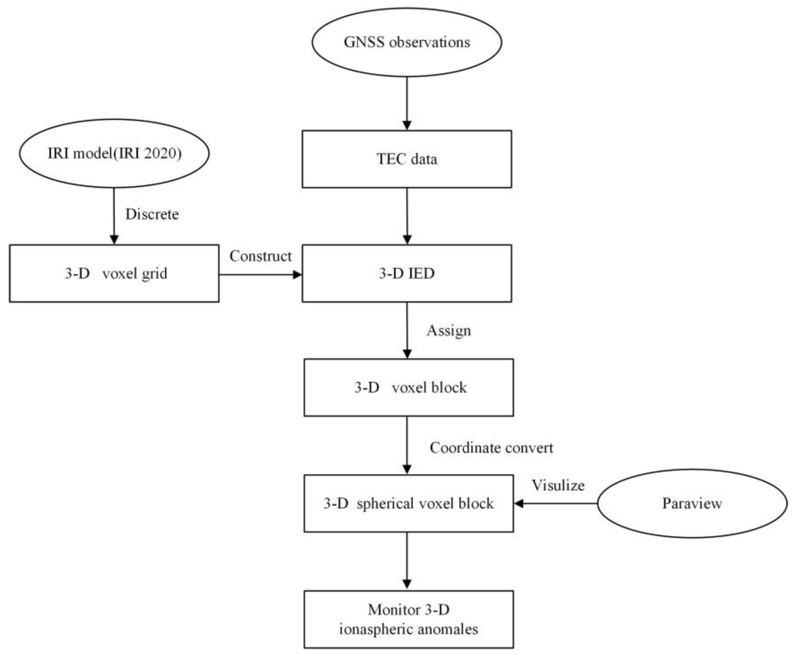
2.2. Method

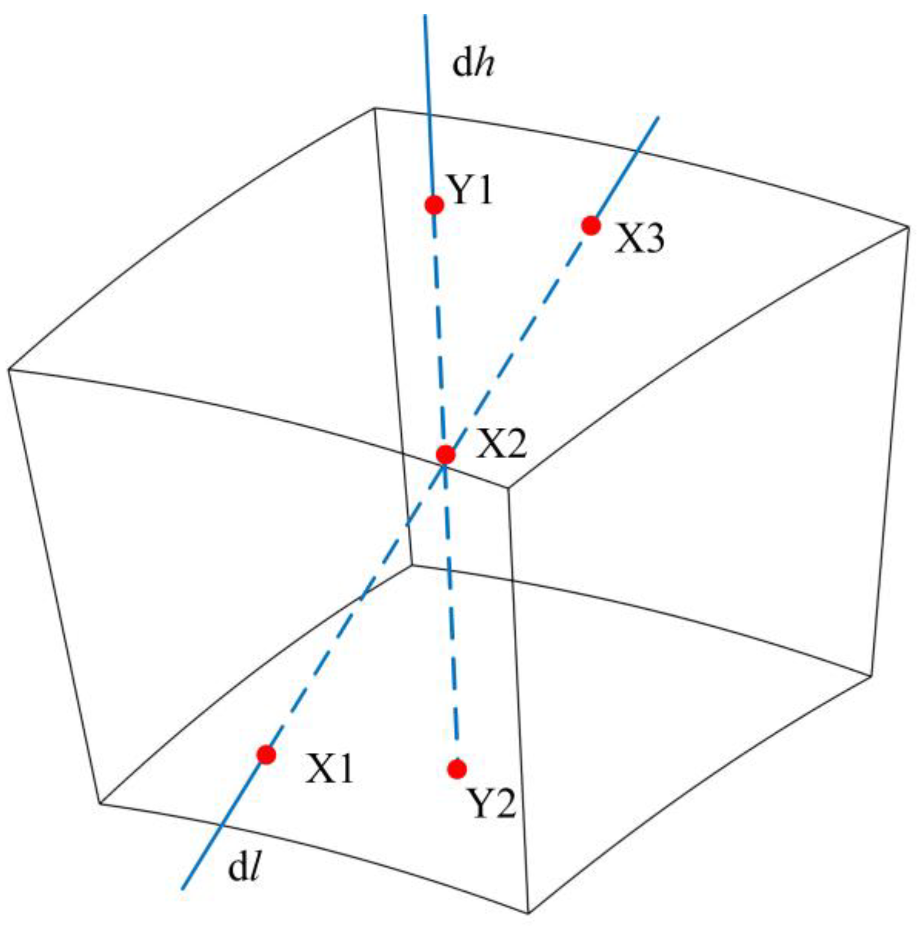
2.2.1. Node-Based Parameterization Tomography

The fundamental relationship between the total electron content (TEC) and electron density in ionospheric tomography is mathematically represented as follows:

$${\mathrm{S}\mathrm{T}\mathrm{E}\mathrm{C}}_{X_1{X}_3}={\int }_{X_1}^{X_3}{N}_e·dl$$

(1)

where $N_e$ denotes the electron density along the signal propagation path $dl$ through the ionosphere. Conventional voxel-based reconstruction methodologies presume a homogeneous electron density distribution within the discrete voxel grid. The direct evaluation of this integral proves computationally prohibitive, necessitating numerical approximation techniques such as the Newton–Gauss algorithm, which require significant computational resources. To overcome these limitations, Chen introduced an improved approach [4]. As illustrated in Figure 1, through the integration of $N_e$ along the ray path $X_1-X_3$ intercepted by voxels, the ${\mathrm{S}\mathrm{T}\mathrm{E}\mathrm{C}}_{X_1{X}_3}$ can be reformulated as follows:

$${\mathrm{S}\mathrm{T}\mathrm{E}\mathrm{C}}_{X_1{X}_3}={\int }_{X_1}^{X_3}{\displaystyle \frac{d\mathrm{V}\mathrm{T}\mathrm{E}\mathrm{C}}{\mathrm{c}\mathrm{o}\mathrm{s}\left(\mathrm{e}\mathrm{l}\mathrm{e}\right)}}$$

(2)

where $d\mathrm{V}\mathrm{T}\mathrm{E}\mathrm{C}$ denotes the vertical total electron content (VTEC) and $\mathrm{e}\mathrm{l}\mathrm{e}$ denotes the elevation angle of $dl$.

After decomposing $d\mathrm{V}\mathrm{T}\mathrm{E}\mathrm{C}$, it can be observed that the horizontal component value is zero, while the vertical component value corresponds to the integral over the height from the lower limit $Y_2$ to the upper limit $Y_1$. Assuming minimal elevation angle variation within individual voxels and that its value can be defined as the elevation angle of $X_2$, Equation (2) reduces to the following:

$${\mathrm{S}\mathrm{T}\mathrm{E}\mathrm{C}}_{X_1{X}_3}={\displaystyle \frac{1}{\mathrm{c}\mathrm{o}\mathrm{s}\left(\mathrm{e}le\right)}}{\int }_{Y_2}^{Y_1}\rho ·dh$$

(3)

Here, $Y_1$ and $Y_2$ correspond to orthogonal projections of observation point $X_2$ onto the voxel’s bounding ellipsoid surfaces, and $dh$ represents the propagation direction of VTEC. In this formulation, ${\mathrm{S}\mathrm{T}\mathrm{E}\mathrm{C}}_{X_1{X}_3}$ can be interpreted as the projection of ${\mathrm{V}\mathrm{T}\mathrm{E}\mathrm{C}}_{Y_1{Y}_2}$ along path $X_1$ to $X_3$. Accounting for the quasi-exponential altitude dependence of IED profiles, the vertical electron density distribution is modeled as follows:

$$Ne={Ne}_{Y_2}·e^{\alpha (h-h_{Y_2})}$$

(4)

where ${Ne}_{Y_2}$ and $h_{Y_2}$ denote the electron density and altitude at $Y_2$, respectively, with α representing the voxel’s exponential IED variation parameter, which is estimated for each voxel from the IRI 2020 IED field [32]. Substitution into Equation (3) yields the following altitude–integrated expression:

$${STEC}_{X_1{X}_3}={\displaystyle \frac{{Ne}_{Y_2}}{\alpha ·\mathrm{c}\mathrm{o}\mathrm{s}\left(\mathrm{e}\mathrm{l}\mathrm{e}\right)}}({Ne}_{Y_2}·(e^{\alpha \left(h_{Y1}-h_{Y_2}\right)}-1)$$

(5)

Through analogous derivation using $Y_1$ as a reference, we obtain the following:

$${STEC}_{X_1{X}_3}={\displaystyle \frac{{Ne}_{Y_1}}{\alpha ·\cos \left(\mathrm{e}\mathrm{l}\mathrm{e}\right)}}(1-{Ne}_{Y_2}·(e^{\alpha \left(h_{Y2}-h_{Y_1}\right)})$$

(6)

Averaging Equations (6) and (7) produces the following:

$${STEC}_{X_1{X}_3}=\left[{Ne}_{Y_2}·e^{\alpha \left(h_{Y1}-h_{Y_2}\right)}-{Ne}_{Y_1}·e^{\alpha \left(h_{Y2}-h_{Y_1}\right)}+{Ne}_{Y_1}-{Ne}_{Y_2}\right]/2·\alpha ·\mathrm{c}\mathrm{o}\mathrm{s}\left(\mathrm{e}\mathrm{l}\mathrm{e}\right)$$

(7)

The electron density (${Ne}_{Y_1}$, ${Ne}_{Y_2}$) is determined through combined vertical exponential and horizontal bilinear interpolation from eight nodal values (${Ne}_{Dk}$, $k$ = 1, …, 8). For instance, ${Ne}_{Y_1}$ is computed as follows:

$${Ne}_{Y_1}=V_1·\sum _{k=1}^4{H}_k{Ne}_{Dk}+V_2·\sum _{k=5}^8{H}_k{Ne}_{Dk}$$

(8)

where $V_1$ and $V_2$ are the coefficients of the vertically exponential interpolation, and $H_k$ ($k$ = 1, 2, …, 8) is the coefficients of the horizontally bilinear interpolation. For details about the interpolation coefficients, refer to Chen. For a generic ray, its STEC can be expressed as a summation of all the intercepts’ STEC. By stacking all the possible STEC measurements together, the matrix form is established as follows:

$$\mathrm{Y}=\mathrm{A}·\mathrm{X}$$

(9)

where Y is the vector of observed STECs, A is the design matrix consisting of elements denoting the contributions of x to the STECs, and X is the vector containing the unknown IED of all voxel nodes. The elements in design matrix A are derived from Equations (7) and (8) and their linear relationship with the eight neighboring nodes. The A matrix is often not squared, ill posed and ill conditioned. In this study, the MART algorithm was used to solve the ill problem. For the $k$-th iteration, the ratio between the observed $\mathrm{Y}$ and reconstructed A, $x^{k-1}$, is calculated to derive corrections for voxel nodes. Specifically, the correction for the $j$-th voxel node from the $i$-th ray in the kth MART iteration is given by the following formula:

$$x_j^k=x_j^{k-1}·{\left({\displaystyle \frac{y_i}{A_i,x^{k-1}}}\right)}^{{\displaystyle \frac{\mu A_{ij}{x}^{k-1}}{{\sum }_{j=1}^n{A}_{ij}{x}^{k-1}}}}$$

(10)

where $\mu$ is the relaxation parameter that adjusts the update step size during each iteration and that is empirically set to 0.9 in our study since it converges efficiently within the short time [33]. This methodology eliminates the numerical integration requirements for tomography equation linearization, significantly reducing the computational complexity. For more details, refer to Chen [34].

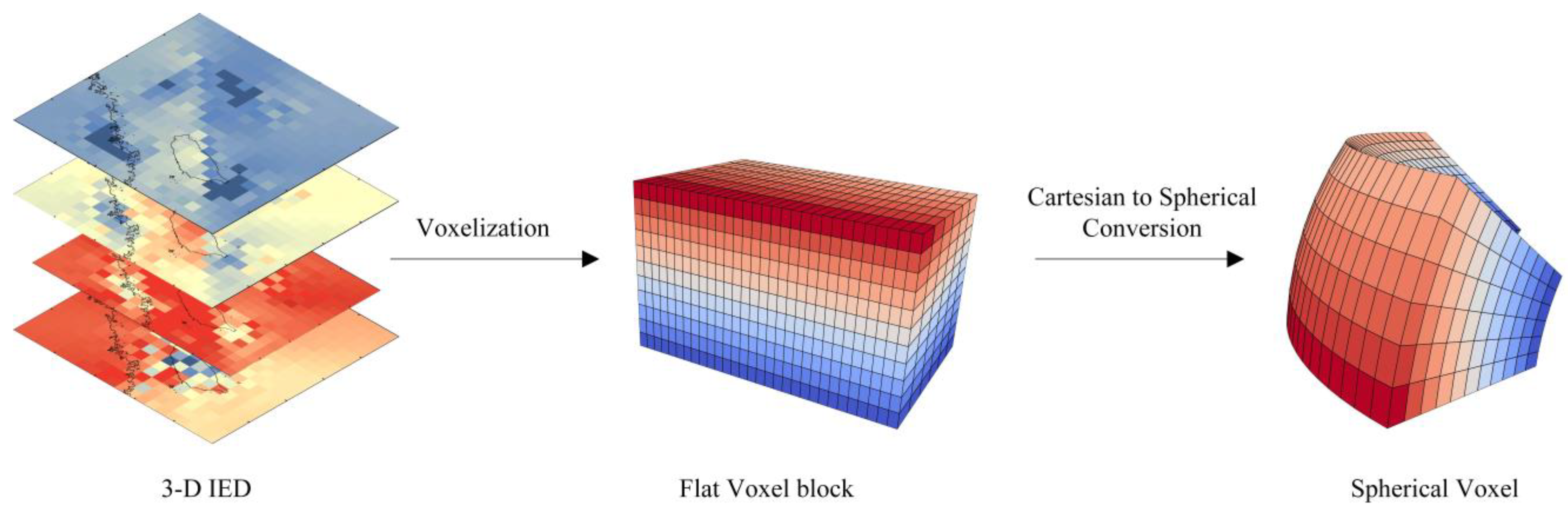
2.2.2. Visualization Model

Traditional mapping tools typically operate within Cartesian coordinate systems in Euclidean space. However, the ionospheric electron density distribution in the real atmosphere exists across curved spherical geometries, necessitating the use of spherical coordinate systems with arc characteristics for accurate 3-D representation. Building upon the concept of Earth system spatial grids (ESSGs), any terrestrial object or phenomenon can be conceptualized as information embedded within such grids [16].

These grids can be comprehensively represented either as an object-based model (left) or field-based model (right), with each grid cell containing spatiotemporal coordinates and associate attributes (Figure 2). The parameters L, T, and A, respectively, denote the location, time, and attributes of entities or phenomena. As for the object model, it abstracts geographic entities into discrete “objects” (points, lines, faces, volumes), each with independent attributes and spatial relationships. Meanwhile, the field model regards geographic space as a continuously distributed “field”, with each location corresponding to an attribute value (such as temperature, electron density, geostress, etc.). Through temporal and spatial resampling aligned with the remote sensing data resolution, all geospatial data can be demonstrated at appropriate levels through the triple elements: location (L), time (T), and attribute (A) [35]. The framework demonstrates the ability to characterize 3-D variations in large-scale Earth system phenomena, making it particularly well suited to modeling the spatiotemporal dynamics of the ionosphere electron density, which can be effectively represented through the application of a field-based model.

The construction of ESSGs involves complex processes including discretization, encoding, coordinate transformation, and visualization. This study employs a simplified longitude–latitude grid system with hexahedral representation. This approach offers computational advantages through its straightforward discretization, which maintains geometric consistency with longitude, latitude and elevation while achieving direct correspondence with a voxels-based grid in tomography. (For distinction, voxels in tomography models are referred to as voxel grids, and the voxel model used in visualization is voxel blocks). However, the method exhibits inherent limitations in polar regions where grid shrinkage leads to data redundancy.

The workflow comprises three primary phases: First, the ionospheric electron density is calculated through a node-based parameter model, where the spatial extent and granularity initial voxel blocks are determined through a tomographic voxel grid. Second, the 3-D ionospheric electron density (IED) data are subsequently mapped into structured 3-D voxel blocks through a voxelization process. Third, spherical coordinate transformation is applied to convert the flat voxel blocks into curvilinear spherical voxel blocks by using Formulas (11)–(13). The final outputs enable visualization and anomaly detection through standard scientific packages such as ParaView or VisIt, as illustrated in Figure 3.

$$x=dr·cos\left(lat\right)·cos\left(lon\right)$$

(11)

$$y=dr·cos\left(lat\right)·sin\left(lon\right)$$

(12)

$$z=dr·sin\left(lat\right)·cos\left(lon\right)$$

(13)

where $lon$, $lat$ and $dr$ are the longitude, latitude and altitude of each voxel. $x$, $y$ and $z$ are the spherical representation of latitude, longitude, and elevation in the Cartesian coordinate system of each voxel.

The flow chart of the visualization framework is shown in Figure 4. The 3-D voxel block is the basic unit in the visualization model, which is constructed based on the location of the voxel grid, representing the 3-D spatial embodiment of voxel grids in the tomography model. Each voxel block represents the electron density at a certain position corresponding to the voxel grid. Assign is the process of assigning electron density to these blocks according to the coordinates.

3. Result

In this study, the 2024 Hualien M7.4 earthquake and the 2023 geomagnetic storm are selected for visualization analysis. The spatial and temporal resolutions are set according to the specific research requirements for each event. For the Hualien earthquake, a geographical domain spanning 118–128° E, 20–30° N, and 100–1000 km is established. Considering an analysis of the fine variations in ionospheric disturbances at a scale of 50–100 km in the epicenter area, the tomographic model is constructed using 0.5° × 0.5° × 50 km grids, resulting in 8379 discrete voxels. Considering the lagged effects associated with lithospheric rupture-induced ionospheric variations, the temporal resolution is maintained at 30 min intervals to effectively capture such ionospheric anomalies. As for the geomagnetic storm, a study area covering 125–66° W and 28–50° N and 100–1000 km is established. A coarser grid of 2° × 1° × 50 km is implemented because IED displays greater variability in the longitude direction than in the latitude direction to accommodate larger-scale ionospheric variations, generating 11,484 discrete voxels. With regard to the temporal resolution, because the rapid electron density variations induced by solar flare disturbances during magnetic storms may occur within minutes to tens of minutes, a 5 min resolution is selected to effectively monitor such dynamic processes [36].

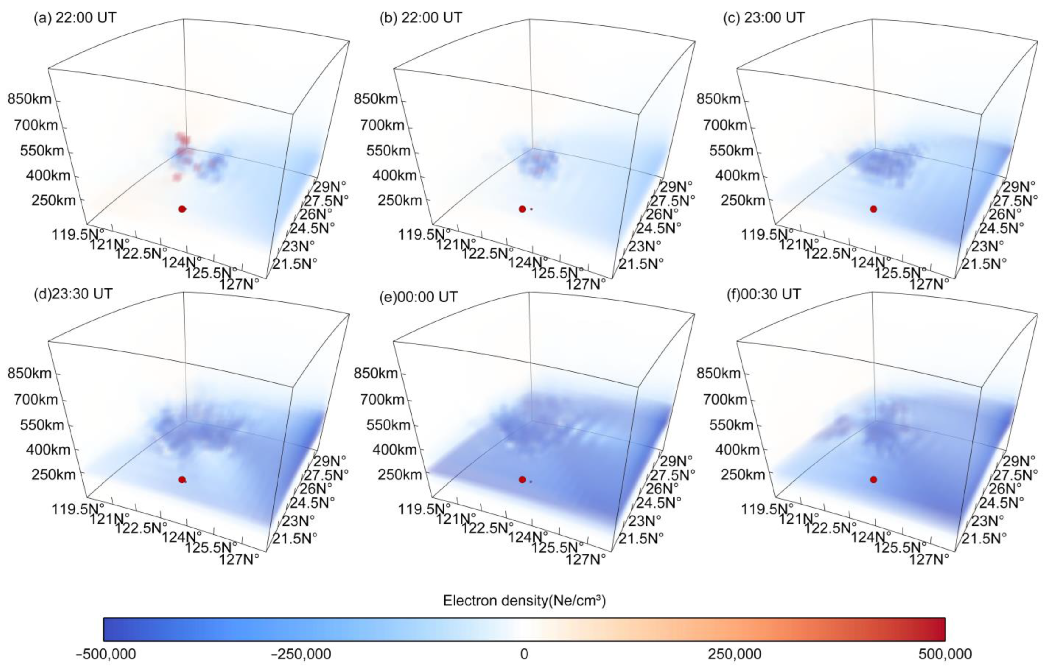
3.1. Case 1: Earthquake Anomaly Analysis via Spherical 3D Tomographic Ne Visualization

A 7.4 magnitude earthquake at a depth of 40 km occurred off the eastern coast of Taiwan, China, at 23:58:12 UTC on 2 April 2024, with the epicenter located at 23.832° N, 121.604° E (Figure 5). Previous studies utilizing multi-source data (ground-based, satellite, and aerial observations) have revealed distinct ionospheric disturbances associated with this seismic event [5]. Here, we employ the anomalous variations in the ionospheric electron density as a case study. The 3-D visualization model of the ionosphere is conducted through tomographic inversion results.

The 3-D ionospheric electron density distribution within the voxel block and slices are presented in Figure 6 and Figure S1, respectively. The results demonstrate a distinct electron density depletion process. A westward-propagating depletion region emerges at a ~200 km altitude across the entire longitudinal sector, persisting throughout the observation period. Simultaneously, a concentrated depletion zone is identified between altitudes of 200 and 400 km above the seismic epicenter (approximately 121–124° E, 23–25° N). This depletion intensifies progressively, reaching maximum severity at 24:00 UT before subsequent attenuation. Specifically, at 22:00 UT (Figure 6a), extensive contiguous positive anomalies with an average of $4.18\times {10}^4\mathrm{N}\mathrm{e}/{\mathrm{c}\mathrm{m}}^3$ are observed southwest of the epicenter at a 200 km altitude. Simultaneously, large-scale negative anomalies dominate the eastern sector between altitudes of 250 and 400 km, with an average of $-1.99\times {10}^5\mathrm{N}\mathrm{e}/{\mathrm{c}\mathrm{m}}^3$. Discontinuous positive anomalies with an average of $6.78\times {10}^5\mathrm{N}\mathrm{e}/{\mathrm{c}\mathrm{m}}^3$ are detected at varying altitudes in the northwest of the epicenter, concurrent with emerging negative anomalies. From 22:30 to 23:30 UT (Figure 6b–d), the northwest positive anomalies transition to negative anomalies (−9.2 $\times {10}^4$ to −1.54 $\times {10}^5\mathrm{N}\mathrm{e}/{\mathrm{c}\mathrm{m}}^3$). This newly formed negative anomaly cluster begin to spread to the surrounding area, while the eastern negative anomalies propagate westward with decreasing intensity gradients (higher values eastward, lower westward). The depletion process culminates with an average of −1.71 $\times {10}^5\mathrm{N}\mathrm{e}/{\mathrm{c}\mathrm{m}}^3$ at 24:00 UT on 2 April (Figure 6e), when both the negative anomaly cluster and the migrating eastern anomalies reach peak intensities, achieving near-complete spatial overlap. By 00:30 UT on 3 April (Figure 6f), the large-scale negative anomalies begin to disappear, accompanied by the weakening of the negative anomaly cluster at the same time.

3.2. Case 2: Geomagnetic Anomaly Analysis via Spherical 3D Tomographic Ne Visualization

The year 2023 demonstrated a period of elevated geomagnetic activity during the current solar cycle. Previous studies utilizing multi-source data analyses demonstrated that severe ionospheric disturbances induced by a geomagnetic storm occurred on 24 April 2024 (Figure 7) [4]. Therefore, the ionospheric perturbation results for 24 April 2024 were selected for visualization modeling analysis.

The three-dimensional IED distributions within spheroidal voxel blocks and slices are illustrated in Figure 8 and Figure S2, respectively. The results reveal a distinct electron density depletion process. The regional anomalies are classified into two distinct layers: a positive anomaly spanning a 200–500 km altitude, extending from 92° W to 68° W and 30° N–40° N. As for the negative anomaly, it almost covers the entire study area at an altitude of 200–250 km. Temporospatial analysis demonstrates southeastward migration and the gradual attenuation of positive anomalies, whereas negative anomalies exhibit a distinct southwestward propagation originating from the northeast. Specifically, the evolution of positive anomalies is categorized into three phases. Phase 1: from 00:00 to 00:30 UT, the initial decay of the positive anomaly intensity is accompanied by southeastward displacement with an average ranging from $5.99\times {10}^4\mathrm{N}\mathrm{e}/{\mathrm{c}\mathrm{m}}^3$ to $4.15\times {10}^4\mathrm{N}\mathrm{e}/{\mathrm{c}\mathrm{m}}^3$, decreasing quickly by about 30.7%. Phase 2: from 00:40 to 01:30, the positive anomalies gradually reduce, reaching their minimum at 1:30 with an average ranging from $3.12\times {10}^4\mathrm{N}\mathrm{e}/{\mathrm{c}\mathrm{m}}^3$ to $2.16\times {10}^4\mathrm{N}\mathrm{e}/{\mathrm{c}\mathrm{m}}^3$, dropping by about 30.8%. Phase 3: From 01:40 to 01:50, the localized resurgence of positive anomalies occurs near 84° W, 40° N, with an average ranging from $2.33\times {10}^4\mathrm{N}\mathrm{e}/{\mathrm{c}\mathrm{m}}^3$ to $2.64\times {10}^4\mathrm{N}\mathrm{e}/{\mathrm{c}\mathrm{m}}^3$, increasing by about 13.9%. Regarding negative anomalies, there are no distinct changes in the spatiotemporal distribution of IED. Negative anomalies demonstrate a small southwestward migration from northeast. At 00:00 UT, negative anomalies are concentrated in the northeastern region, with continued migration toward the southwestern sector from 00:00 to 01:50, accompanied by the enhancing negative anomalies ($-1.02\times {10}^5$ to $-1.34\times {10}^5\mathrm{N}\mathrm{e}/{\mathrm{c}\mathrm{m}}^3$).

4. Discussion

Compared to traditional ionospheric tomography methods, node-based parameterization can theoretically reconstruct the IED at any spatial scale. Quantitative analyses from prior research indicate that this methodology achieves a significant accuracy enhancement of 10–40% relative to traditional reconstruction approaches when addressing ionospheric structure characterization [4,34]. As for the results, there are negative anomalies advancing from northeast to southwest at an altitude of 200 km in both cases, accompanied by ionospheric disturbance appearing above the negative anomalies. It is obvious that the large-scale negative anomaly propagation is the change in the background field. In earthquakes, the changes in negative anomalies are bottom-up, and when they reach a height of almost 200 km, there is an overlap with the changes in the background field during the evolution process. On the contrary, in geomagnetic storms, anomalies are top-down, and always remain above the background field. This phenomenon suggests that ionospheric negative anomalies in earthquakes are attributed to internal Earth processes, whereas ionospheric disturbances associated with geomagnetic storms are predominantly induced by external solar activities in the space environment. A fundamental difference in the triggering mechanisms is observed: the former represents geophysical effects driven by endogenous forces, while the latter constitutes space weather phenomena resulting from exogenous perturbations. This differentiation provides critical evidence for explaining the genesis of various ionospheric anomalies, confirming that internal tectonic activities and external space environmental disturbances exhibit distinct driving mechanisms in ionospheric variations.

4.1. Analysis of Ionospheric Disturbance of the Earthquake Case

In the Hualien earthquake case study, a pronounced negative anomaly cluster exhibiting peak intensity at the seismic origin time was identified directly above the epicenter, gradually dissipating over time. Figure 6 illustrates the emergence of negative anomalies from the Earth’s surface, which subsequently propagate upward within the 200–400 km altitude range over time, while continuously diffusing laterally during their ascent. The observed vertical upward propagation of ionospheric depletion signatures, coupled with the spatiotemporal correlation with seismic precursors, could suggest that the persistent negative anomaly region originates from pre-seismic stress-induced lithosphere–atmosphere–ionosphere coupling (LAIC) mechanisms [37]. Tectonic plate movements and crustal stress accumulation constitute the fundamental causes of ionospheric negative anomalies [38], which may manifest through multiple geophysical interaction mechanisms, such as acoustic-gravity waves [39], atmospheric electric fields [40] and gas effects [41] (such as radon and carbon dioxide). In this study, it is inferred that the negative anomalies could be caused by the convergence of positive charge carriers and electrons. This is where crustal rupture releases positive charge carriers that subsequently penetrate into the ionosphere through atmospheric electric fields. The recombination of these positive charges with electrons ultimately leads to the observed reduction in electron density within the ionosphere [42].

In addition, the 3D model further demonstrates an enhanced ability to identify non-seismic anomalies. Figure 6 demonstrates that the negative anomaly at the altitude of ~200 km intensifies progressively from east to west over time, accompanied by a gradual east-to-west migration. In addition, three-dimensional modeling reveals a distinct formation between the previously described negative anomaly cluster and this evolving anomaly, with a high probability that this large-scale anomaly is not caused by the earthquake.

4.2. Analysis of Ionospheric Disturbance of the Geomagnetic Storm Case

The method depicts the large-scale electron density depletion processes associated with geomagnetic storms. Three distinct phases are observed in the temporal evolution of positive anomalies within the study region. During phase 1, the positive anomaly decreased rapidly, with a 30.6% density reduction within 30 min. This was followed by a protracted depletion phase 2, where the electron density gradually decreased by 30.7% over the subsequent hour. Phase 3 experienced a 13.9% increase in electron density within 10 min. With regard to the negative anomalies, the electron density continued to decrease throughout the stage. In general, both positive and negative anomalies exhibit a persistent reduction in electron density, which could be caused by geomagnetic storms. There are various physical mechanisms by which geomagnetic storms cause electron density decay [36], and generally speaking, in mid-latitude regions, they are highly likely to be affected by the effect of neutral composition changes [43,44]. The initiation of geomagnetic disturbances triggers the formation of molecular compositional bulge within the auroral oval, which is subsequently transported to lower latitudes by neutral winds. Such rapid neutral atmospheric expansion is hypothesized to induce upwelling, followed by a sharp decline in the neutral density ratios of O/N₂ and O/O₂. Consequently, this alteration results in the depletion of electron density [45].

5. Conclusions

In this article, a rapid visualization modeling framework employing the DGGS concept is developed to transform 3-D IED into spheroidal voxel representations, enabling the 3-D visualization and analysis of electron density variations across multiple altitudes. Compared with conventional ionospheric slice analyses, the proposed voxel-based approach effectively discriminates spatiotemporal variations in positive/negative anomalies at different altitudes, thereby facilitating the differentiation of ionospheric perturbations caused by major geophysical events (e.g., seismic activity) and space weather phenomena (e.g., geomagnetic storms). In addition, our visualization model demonstrates distinct propagation patterns across varying altitudes within identical geospatial coordinates. Notably, in practical situations, areas with higher elevations in the same geospatial coordinates occupy a larger area. This critical spatial characteristic is accurately captured by our visualization framework, whereas conventional slice-based approaches fail to adequately represent such three-dimensional features. Furthermore, due to the expression of the field model, the origin of ionospheric anomalies caused by large-scale events can be clearly distinguished, which may provide a solution for identifying ionosphere anomalies.

However, some limitations remain: (i)Although it is a 3-D model, the results are demonstrated through two-dimensional images, which may result in potential visual inaccuracies to some extent. (ii) Due to our 3-D model, the results from different positions in 3-D space may overlap and cause confusion. (iii) The latitudinal–longitudinal grid, though compatible with the voxel-based tomograph, suffers from progressive shrinkage in polar regions, reducing its efficacy for high-latitude applications. Future research should focus on the overlay problem associated with 3-D representation, which may be solved through visualization algorithms. As the shrinkage grid in polar regions, adaptively adjusting the grid size based on the research area may be a solution.

References

- Jin, X.; Song, S.; Zhou, W.; Cheng, N. Multi-GNSS global ionosphere modeling enhanced by virtual observation stations based on IRI-2016 model. J. Geod. 2022, 96, 81. [Google Scholar] [CrossRef]
- Yao, Y.; Kong, J.; Tang, J. A New Ionosphere Tomography Algorithm With Two-Grid Virtual Observations Constraints and Three-Dimensional Velocity Profile. IEEE Trans. Geosci. Remote Sens. 2015, 53, 2373–2383. [Google Scholar] [CrossRef]
- Yao, Y.; Zhai, C.; Kong, J.; Zhao, C.; Luo, Y.; Liu, L. An improved constrained simultaneous iterative reconstruction technique for ionospheric tomography. GPS Solut. 2020, 24, 68. [Google Scholar] [CrossRef]
- Chen, B.; Wang, X.; Zhang, Z.; Jin, L.; Yu, W. Time-Dependent Ionospheric Tomography Based on Two-Step Reconstruction and Node Parameterization Algorithm. IEEE J. Sel. Top. Appl. Earth Obs. Remote Sens. 2024, 17, 15789–15805. [Google Scholar] [CrossRef]
- Wu, D.; Xie, B.; Chen, B.; Rasheed, R.; Wu, L. Characteristics of Potential Ionospheric Anomalies Prior to the M7.4 April 2, 2024 Taiwan Earthquake Identified With Multiple Observations. IEEE Geosci. Remote Sens. Lett. 2024, 21, 1003605. [Google Scholar] [CrossRef]
- He, L.; Heki, K. Three-Dimensional Tomography of Ionospheric Anomalies Immediately Before the 2015 Illapel Earthquake, Central Chile. J. Geophys. Res. Space Phys. 2018, 123, 4015–4025. [Google Scholar] [CrossRef]
- Hu, T.; Xu, X.; Luo, J. Improving the Computerized Ionospheric Tomography Performance Through a Neural Network-Based Initial IED Prediction Model. IEEE Trans. Geosci. Remote Sens. 2024, 62, 5800117. [Google Scholar] [CrossRef]
- Kao, S.-P.; Chen, Y.-C.; Ning, F.-S.; Tu, Y.-M. An LS-MARS method for modeling regional 3D ionospheric electron density based on GPS data and IRI. Adv. Space Res. 2015, 55, 2256–2267. [Google Scholar] [CrossRef]
- Hirooka, S.; Hattori, K.; Takeda, T. Numerical validations of neural-network-based ionospheric tomography for disturbed ionospheric conditions and sparse data. Radio Sci. 2011, 46, RS0F05. [Google Scholar] [CrossRef]
- Yao, Y.; Zhai, C.; Kong, J.; Zhao, Q.; Zhao, C. A modified three-dimensional ionospheric tomography algorithm with side rays. GPS Solut. 2018, 22, 107. [Google Scholar] [CrossRef]
- Lu, W.; Ma, G.; Wan, Q. A Review of Voxel-Based Computerized Ionospheric Tomography with GNSS Ground Receivers. Remote Sens. 2021, 13, 3432. [Google Scholar] [CrossRef]
- Zhang, W.; Zhang, S.; Moeller, G.; Qi, M.; Ding, N. An adaptive-degree layered function-based method to GNSS tropospheric tomography. GPS Solut. 2023, 27, 67. [Google Scholar] [CrossRef]
- Haji-Aghajany, S.; Amerian, Y.; Verhagen, S.; Rohm, W.; Schuh, H. The effect of function-based and voxel-based tropospheric tomography techniques on the GNSS positioning accuracy. J. Geod. 2021, 95, 78. [Google Scholar] [CrossRef]
- Cahyadi, M.N.; Arisa, D.; Muafiry, I.N.; Muslim, B.; Rahayu, R.W.; Putra, M.E.; Wulansari, M. Three-Dimensional Tomography of Coseismic Ionospheric Disturbances Following the 2018 Palu Earthquake and Tsunami from GNSS Measurements. Front. Astron. Space Sci. 2022, 9, 890603. [Google Scholar] [CrossRef]
- Prol, F.S.; Kodikara, T.; Hoque, M.M.; Borries, C. Global-Scale Ionospheric Tomography During the March 17, 2015 Geomagnetic Storm. Space Weather 2021, 19, e2021SW002889. [Google Scholar] [CrossRef]
- Yu, J.Q.; Wu, L.X.; Jia, Y.J. ESSG-based global spatial reference frame for datasets interrelation. Int. Arch. Photogramm. Remote Sens. Spat. Inf. Sci. 2013, XL-4/W2, 57–62. [Google Scholar] [CrossRef]
- Goodchild, M.F. Reimagining the history of GIS. Ann. GIS 2018, 24, 1–8. [Google Scholar] [CrossRef]
- Ma, T.; Zhou, C.; Xie, Y.; Qin, B.; Ou, Y. A discrete square global grid system based on the parallels plane projection. Int. J. Geogr. Inf. Sci. 2009, 23, 1297–1313. [Google Scholar] [CrossRef]
- Li, Q.; Chen, X.; Tong, X.; Zhang, X.; Cheng, C. An Information Fusion Model between GeoSOT Grid and Global Hexagonal Equal Area Grid. ISPRS Int. J. Geo-Inf. 2022, 11, 265. [Google Scholar] [CrossRef]
- Wang, R.; Ben, J.; Du, L.; Zhou, J.; Li, Z. Code Operation Scheme for the Icosahedral Aperture 4 Hexagonal Grid System. Geomat. Inf. Sci. Wuhan Univ. 2020, 45, 89–96. [Google Scholar] [CrossRef]
- Li, M.; McGrath, H.; Stefanakis, E. Multi-resolution topographic analysis in hexagonal Discrete Global Grid Systems. Int. J. Appl. Earth Obs. Geoinf. 2022, 113, 102985. [Google Scholar] [CrossRef]
- Wagner, S.; Stenzel, F.; Krueger, T.; de Wiljes, J. Drivers of global irrigation expansion: The role of discrete global grid choice. Hydrol. Earth Syst. Sci. 2024, 28, 5049–5068. [Google Scholar] [CrossRef]
- Lu, F.; Konecny, M.; Chen, M.; Reznik, T. A Barotropic Tide Model for Global Ocean Based on Rotated Spherical Longitude-Latitude Grids. Water 2021, 13, 2670. [Google Scholar] [CrossRef]
- He, L.M.; Yang, Y.; Su, C.; Yu, J.Q.; Yang, F.; Wu, L.X. Grid-based representation and dynamic visualization of ionospheric tomography. Int. Arch. Photogramm. Remote Sens. Spat. Inf. Sci. 2013, XL-4/W2, 71–76. [Google Scholar] [CrossRef]
- Wu, L.X.; Yu, J.Q.; Yang, Y.Z.; Jia, Y.J. Spatial Big Data Organization, Access and Visualization with ESSG. Int. Arch. Photogramm. Remote Sens. Spat. Inf. Sci. 2013, XL-4/W2, 51–56. [Google Scholar] [CrossRef]
- Zhang, B.; Ou, J.; Yuan, Y.; Li, Z. Extraction of line-of-sight ionospheric observables from GPS data using precise point positioning. Sci. China Earth Sci. 2012, 55, 1919–1928. [Google Scholar] [CrossRef]
- Wang, J.; Huang, G.; Zhou, P.; Yang, Y.; Zhang, Q.; Gao, Y. Advantages of Uncombined Precise Point Positioning with Fixed Ambiguity Resolution for Slant Total Electron Content (STEC) and Differential Code Bias (DCB) Estimation. Remote Sens. 2020, 12, 304. [Google Scholar] [CrossRef]
- Ren, X.; Chen, J.; Li, X.; Zhang, X. Ionospheric Total Electron Content Estimation Using GNSS Carrier Phase Observations Based on Zero-Difference Integer Ambiguity: Methodology and Assessment. IEEE Trans. Geosci. Remote Sens. 2021, 59, 817–830. [Google Scholar] [CrossRef]
- Xie, T.; Chen, B.; Wu, L.; Dai, W.; Kuang, C.; Miao, Z. Detecting Seismo-Ionospheric Anomalies Possibly Associated With the 2019 Ridgecrest (California) Earthquakes by GNSS, CSES, and Swarm Observations. J. Geophys. Res. Space Phys. 2021, 126, e2020JA028761. [Google Scholar] [CrossRef]
- He, R.; Li, M.; Zhang, Q.; Zhao, Q. A Comparison of a GNSS-GIM and the IRI-2020 Model Over China Under Different Ionospheric Conditions. Space Weather 2023, 21, e2023SW003646. [Google Scholar] [CrossRef]
- JIN, L.; CHEN, B.; WANG, X.; WU, D. Global Accuracy Assessment and Analysis of the Ionospheric Model IRI-Plas 2020 and IRI-2020 Based on GNSS Observations. Chin. J. Space Sci. 2024, 44, 1031–1046. [Google Scholar] [CrossRef]
- Alizadeh, M.M.; Schuh, H.; Schmidt, M. Ray tracing technique for global 3-D modeling of ionospheric electron density using GNSS measurements. Radio Sci. 2015, 50, 539–553. [Google Scholar] [CrossRef]
- Chen, B.; Jin, L.; Wang, J.; Jin, W.; Wang, W. Wide-Area Retrieval of Water Vapor Field Using an Improved Node Parameterization Tomography. IEEE Geosci. Remote Sens. Lett. 2023, 20, 1001805. [Google Scholar] [CrossRef]
- Chen, B.; Wu, L.; Dai, W.; Luo, X.; Xu, Y. A new parameterized approach for ionospheric tomography. GPS Solut. 2019, 23, 96. [Google Scholar] [CrossRef]
- Yu, J.; Wu, L.; Li, Z.; Li, X. An SDOG-based intrinsic method for three-dimensional modelling of large-scale spatial objects. Ann. GIS 2012, 18, 267–278. [Google Scholar] [CrossRef]
- Afraimovich, E.L.; Boitman, O.N.; Zhovty, E.I.; Kalikhman, A.D.; Pirog, T.G. Dynamics and anisotropy of traveling ionospheric disturbances as deduced from transionospheric sounding data. Radio Sci. 1999, 34, 477–487. [Google Scholar] [CrossRef]
- Nayak, K.; Romero-Andrade, R.; Sharma, G.; Zavala, J.L.C.; Urias, C.L.; Trejo Soto, M.E.; Aggarwal, S.P. A combined approach using b-value and ionospheric GPS-TEC for large earthquake precursor detection: A case study for the Colima earthquake of 7.7 Mw, Mexico. Acta Geod. Geophys. 2023, 58, 515–538. [Google Scholar] [CrossRef]
- Sharma, G.; Nayak, K.; Romero-Andrade, R.; Aslam, M.A.M.; Sarma, K.K.; Aggarwal, S.P. Low Ionosphere Density Above the Earthquake Epicentre Region of Mw 7.2, El Mayor–Cucapah Earthquake Evident from Dense CORS Data. J. Indian Soc. Remote Sens. 2024, 52, 543–555. [Google Scholar] [CrossRef]
- Meng, X.; Verkhoglyadova, O.P.; Komjathy, A.; Savastano, G.; Mannucci, A.J. Physics-Based Modeling of Earthquake-Induced Ionospheric Disturbances. J. Geophys. Res. Space Phys. 2018, 123, 8021–8038. [Google Scholar] [CrossRef]
- Wu, L.; Wang, X.; Qi, Y.; Lu, J.C.; Mao, W. Characteristics and mechanisms of near-surface atmospheric electric field 1 negative anomalies preceding the 5 September, 2022, Ms6.8 Luding earthquake. Nat. Hazards Earth Syst. Sci. 2024, 24, 773–789. [Google Scholar]
- Liu, Y.; Wu, L.; Qi, Y.; Ding, Y. General features of multi-parameter anomalies of six moderate earthquakes occurred near Zhangbei-Bohai fault in China during the past decades. Remote Sens. Environ. 2023, 295, 113692. [Google Scholar] [CrossRef]
- Wu, L.; Qi, Y.; Mao, W.; Lu, J.; Ding, Y.; Peng, B.; Xie, B. Scrutinizing and rooting the multiple anomalies of Nepal earthquake sequence in 2015 with the deviation–time–space criterion and homologous lithosphere–coversphere–atmosphere–ionosphere coupling physics. Nat. Hazards Earth Syst. Sci. 2023, 23, 231–249. [Google Scholar] [CrossRef]
- Afraimovich, E.L.; Astafyeva, E.I.; Demyanov, V.V.; Gamayunov, I.F. Mid-latitude amplitude scintillation of GPS signals and GPS performance slips. Adv. Space Res. 2009, 43, 964–972. [Google Scholar] [CrossRef]
- Vijaya Lekshmi, D.; Balan, N.; Tulasi Ram, S.; Liu, J.Y. Statistics of geomagnetic storms and ionospheric storms at low and mid latitudes in two solar cycles. J. Geophys. Res. Space Phys. 2011, 116, A11328. [Google Scholar] [CrossRef]
- Feng, J.; Zhou, Y.; Zhou, Y.; Gao, S.; Zhou, C.; Tang, Q.; Liu, Y. Ionospheric response to the 17 March and 22 June 2015 geomagnetic storms over Wuhan region using GNSS-based tomographic technique. Adv. Space Res. 2021, 67, 111–121. [Google Scholar] [CrossRef]
Disclaimer/Publisher’s Note: The statements, opinions and data contained in all publications are solely those of the individual author(s) and contributor(s) and not of MDPI and/or the editor(s). MDPI and/or the editor(s) disclaim responsibility for any injury to people or property resulting from any ideas, methods, instructions or products referred to in the content. |
© 2025 by the authors. Licensee MDPI, Basel, Switzerland. This article is an open access article distributed under the terms and conditions of the Creative Commons Attribution (CC BY) license (https://creativecommons.org/licenses/by/4.0/).
Share and Cite
Peng, B.; Chen, B.; Xie, B.; Wu, L. Ionospheric Anomaly Identification: Based on GNSS-TEC Data Fusion Supported by Three-Dimensional Spherical Voxel Visualization. Atmosphere 2025, 16, 428. https://doi.org/10.3390/atmos16040428
Peng B, Chen B, Xie B, Wu L. Ionospheric Anomaly Identification: Based on GNSS-TEC Data Fusion Supported by Three-Dimensional Spherical Voxel Visualization. Atmosphere. 2025; 16(4):428. https://doi.org/10.3390/atmos16040428
Chicago/Turabian StylePeng, Boqi, Biyan Chen, Busheng Xie, and Lixin Wu. 2025. "Ionospheric Anomaly Identification: Based on GNSS-TEC Data Fusion Supported by Three-Dimensional Spherical Voxel Visualization" Atmosphere 16, no. 4: 428. https://doi.org/10.3390/atmos16040428
APA StylePeng, B., Chen, B., Xie, B., & Wu, L. (2025). Ionospheric Anomaly Identification: Based on GNSS-TEC Data Fusion Supported by Three-Dimensional Spherical Voxel Visualization. Atmosphere, 16(4), 428. https://doi.org/10.3390/atmos16040428