Modeling Short-Term Drought for SPEI in Mainland China Using the XGBoost Model

Abstract

Accurate drought prediction is crucial for optimizing water resource allocation, safeguarding agricultural productivity, and maintaining ecosystem stability. This study develops a methodological framework for short-term drought forecasting using SPEI time series (1979–2020) and evaluates three predictive models: (1) a baseline XGBoost model (XGBoost1), (2) a feature-optimized XGBoost variant incorporating Pearson correlation analysis (XGBoost2), and (3) an enhanced CPSO-XGBoost model integrating hybrid particle swarm optimization with dual mechanisms of binary feature selection and parameter tuning. Key findings reveal spatiotemporal prediction patterns: temporal-scale dependencies show all models exhibit limited capability at SPEI-1 (R²: 0.32–0.41, RMSE: 0.68–0.79) but achieve progressive accuracy improvement, peaking at SPEI-12 where CPSO-XGBoost attains optimal performance (R²: 0.85–0.90, RMSE: 0.33–0.43) with 18.7–23.4% error reduction versus baselines. Regionally, humid zones (South China/Central-Southern) demonstrate peak accuracy at SPEI-12 (R² ≈ 0.90, RMSE < 0.35), while arid regions (Northwest Desert/Qinghai-Tibet Plateau) show dramatic improvement from SPEI-1 (R² < 0.35, RMSE > 1.0) to SPEI-12 (R² > 0.85, RMSE reduction > 52%). Multivariate probability density analysis confirms the model’s robustness through enhanced capture of nonlinear atmospheric-land interactions and reduced parameterization uncertainties via swarm intelligence optimization. The CPSO-XGBoost’s superiority stems from synergistic optimization: binary particle swarm feature selection enhances input relevance while adaptive parameter tuning improves computational efficiency, collectively addressing climate variability challenges across diverse terrains. These findings establish an advanced computational framework for drought early warning systems, providing critical support for climate-resilient water management and agricultural risk mitigation through spatiotemporally adaptive predictions.

1. Introduction

The escalating complexity of drought regimes under anthropogenic climate change and intensified human activities presents critical challenges for water security, particularly in monsoon-dominated regions with complex topography such as China [1,2,3]. Since the 1970s, drought-affected agricultural areas in China have averaged 20.9 million hectares annually, incurring economic losses exceeding 44 billion CNY, highlighting systemic vulnerabilities in current drought management paradigms [4]. This urgency necessitates the development of advanced predictive frameworks integrating cutting-edge monitoring indices and computational intelligence.

Contemporary drought quantification relies on standardized indices that operationalize meteorological and hydrological processes. The Standardized Precipitation Index establishes precipitation deficit baselines, while the Palmer Drought Severity Index introduces multi-scalar water balance computations [5,6]. The SPEI represents a paradigm advancement through the synergistic integration of precipitation anomalies and potential evapotranspiration, effectively capturing the thermodynamic coupling inherent in modern drought regimes under climate change [6]. SPEI’s capacity to resolve both moisture supply and atmospheric demand dynamics has cemented its dominance in contemporary drought monitoring systems.

Machine learning architectures have revolutionized hydroclimatic prediction through nonlinear pattern recognition capabilities. XGBoost has emerged as a prominent methodology, demonstrating superior performance in comparative analyses against traditional approaches including Distributed Lag Non-linear Models and Artificial Neural Networks [3,7]. Empirical validations reveal XGBoost achieves exceptional predictive skill (R² > 0.85) for SPEI forecasts at 1–6 month lead times, establishing new benchmarks for operational drought early warning systems [3]. Land relief directly influences land use patterns by dictating water retention, soil moisture distribution, and agricultural suitability [8]. For instance, steep slopes in mountainous regions limit arable land, promoting forest cover, while flat plains in North China support intensive croplands vulnerable to irrigation-dependent droughts. These interactions align with findings from Moldova, where spatial analyses of forest–agriculture dynamics using remote sensing and GIS techniques revealed critical trade-offs between crop expansion and forest conservation [9].

Parameter optimization constitutes a critical pathway for enhancing predictive fidelity in complex environmental systems. Conventional optimization strategies—manual hyperparameter tuning, Bayesian optimization, and random search—face intrinsic limitations in high-dimensional parameter spaces characteristic of ensemble learning architectures [10]. Metaheuristic algorithms including PSO and Genetic Algorithms overcome these constraints through stochastic global search mechanisms, effectively balancing exploration–exploitation tradeoffs while mitigating local optima entrapment [11,12]. Implementations in evapotranspiration modeling demonstrate that PSO-optimized XGBoost architectures reduce prediction errors by 18–23% compared to baseline models [13].

Feature space optimization represents an equally critical dimension in drought prediction systems. The selection of physiographically relevant predictors—including vegetation dynamics, thermal stress indicators, and precipitation anomalies—fundamentally governs model generalizability [14]. Drought severity is strongly correlated with land cover types and atmospheric circulation patterns. For example, in Central-South China, prolonged negative phases of the Indian Ocean Dipole reduce rainfall, intensifying droughts in cropland-dominated regions [15]. These dynamics resonate with multi-hazard assessments in North Macedonia, where integrated GIS-based models identified synergistic risks of soil erosion and landslides under climate change, emphasizing the need for adaptive strategies to address compound environmental stressors [8]. While conventional dimensionality reduction techniques (Pearson correlation filters, Principal Component Analysis) inadequately capture nonlinear feature interactions, evolutionary computation approaches such as BPSO enable intelligent feature subspace selection [16]. BPSO-enhanced models demonstrate 27–34% improvement in drought classification accuracy through the optimized representation of land–atmosphere feedback mechanisms.

The current scientific paradigm exhibits a critical limitation in addressing the coupled optimization challenges inherent in environmental forecasting systems, where parameter tuning and feature subspace selection are typically pursued as discrete computational processes. This decoupled approach fundamentally neglects the synergistic interdependencies between model architecture configuration and predictor space composition—a methodological gap that constrains predictive performance in complex hydroclimatic systems. Our study bridges this conceptual divide through the implementation of a Hybrid CPSO architecture that synchronously optimizes XGBoost hyperparameters and feature subspace selection via integrative binary-continuous coding mechanisms [17]. This dual-optimization framework synergistically combines the global search capabilities of PSO with the feature selection prowess of BPSO, achieving concurrent maximization of model structural efficiency and predictive feature relevance.

The CPSO-XGBoost framework has demonstrated transformative potential across multiple environmental forecasting domains. In agricultural systems modeling, CPSO-optimized architectures improved cereal yield prediction accuracy (R² > 0.92) through intelligent integration of meteorological covariates, edaphic parameters, and phenological indicators [18]. Atmospheric science applications reveal similar advancements, where CPSO-enhanced models reduced PM2.5 forecasting errors by 31–38% through the optimal fusion of emission inventories, traffic flow patterns, and boundary layer dynamics [19]. These cross-domain validations confirm the framework’s capacity to resolve multivariate environmental system complexities through coordinated parameter–feature optimization.

Notwithstanding these advancements, the application of CPSO-XGBoost architectures to hydroclimatic extreme prediction remains conspicuously underdeveloped. Our research pioneers the implementation of this integrated optimization framework for multi-timescale SPEI forecasting, employing a comprehensive predictor matrix comprising 19 atmospheric–terrestrial covariates—including key circulation indices, antecedent SPEI states, and geospatial determinants. This systematic integration enables the simultaneous resolution of two critical challenges in drought prediction: (1) optimal parameterization of ensemble learning architectures for hydroclimatic time series, and (2) intelligent selection of physically meaningful predictors across atmospheric-land surface subsystems.

Through this dual-optimization paradigm, our methodology establishes new standards for predictive accuracy and operational stability in drought forecasting systems. By advancing the computational frontiers of machine learning applications in hydroclimatology, this research provides a transformative decision-support platform for climate-resilient water resource management and agricultural contingency planning under intensifying anthropogenic climate change.

In Section 2, we detail the study area, data sources, and methodological framework for model construction and evaluation. Section 3 presents the spatiotemporal performance of the three predictive models across multiple timescales and climatic regions. Section 4 discusses the comparative advantages of the CPSO-XGBoost framework and its implications for drought early warning systems. Finally, Section 5 summarizes the key findings and outlines future research directions.

2. Data and Methods

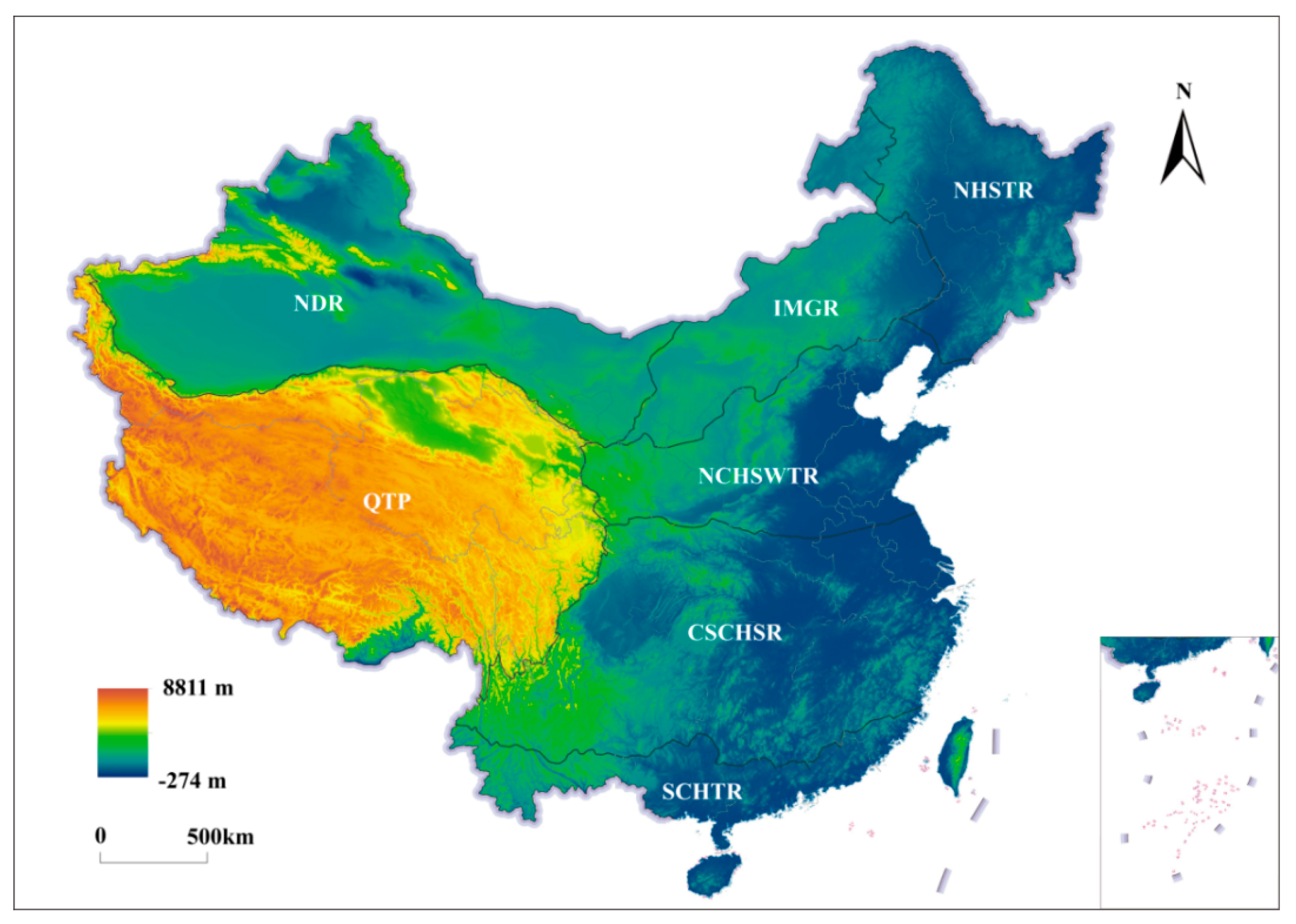
2.1. Study Area and Data Sources

The terrain of mainland China exhibits a distinct west-to-east descending gradient, structured into three topographic tiers [20]. This geographical and climatic diversity has resulted in the classification of the country into seven distinct natural regions [21]: the NDR, the IMGR, the NHSTR, the QTP, the NCHSWTR, the CSCHSR, and the SCHTR (Figure 1).

These regions exhibit significant climatic variability. The NDR is characterized by an arid climate with extremely low precipitation, high evaporation rates, and large temperature differences between day and night, making water scarcity a key constraint. The IMGR has a semi-arid continental climate with cold winters, warm summers, and low but variable precipitation, supporting temperate grasslands that are highly sensitive to drought and desertification. The NHSTR experiences a temperate monsoon climate with cold, dry winters and warm, humid summers, receiving moderate to high precipitation that supports fertile croplands but is vulnerable to seasonal droughts. The QTP, known as the “Roof of the World”, has an alpine climate with low temperatures, strong solar radiation, and widespread permafrost, with summer precipitation playing a crucial role in regional hydrological processes. The NCHSWTR has a warm temperate monsoon climate with hot, humid summers and cold, dry winters, featuring moderate precipitation concentrated in summer and increasing drought risks due to climate variability. The CSCHSR has a humid subtropical monsoon climate with abundant rainfall, high humidity, and mild winters, frequently experiencing typhoons and extreme precipitation events that can lead to both floods and droughts. The SCHTR, with its tropical monsoon climate, has high temperatures and heavy rainfall year-round, featuring distinct wet and dry seasons; while water resources are generally sufficient, occasional prolonged dry spells can still impact agriculture and water supply.

The study integrates two primary datasets: atmospheric circulation indices from the National Oceanic and Atmospheric Administration Climate Data Center (https://psl.noaa.gov/data/climateindices/, accessed on 10 May 2023) and SPEI values from the global SPEI database (https://spei.csic.es/, accessed on 10 May 2023). Monthly circulation indices encompass key climate oscillation patterns detailed in

Table 1. Overview of atmospheric circulation indices.

Index	Full Name	Period (Year)
AMO	Atlantic Multidecadal Oscillation	1856–2022
DMI	Indian Ocean Dipole Mode Index	1870–2022
AO	Arctic Oscillation	1950–2022
ESPI	El Niño–Southern Oscillation Precipitation Index	1979–2022
NAO	North Atlantic Oscillation	1950–2022
MEI	Multivariate ENSO Index	1979–2022
Niño1+2	Average Sea Surface Temperature Anomaly in Niño1 and Niño2 Regions	1950–2022
Niño3.4	Average Sea Surface Temperature Anomaly in the Overlap of Niño3 and Niño4 Regions
Niño3	Average Sea Surface Temperature Anomaly in Niño3 Region
Niño4	Average Sea Surface Temperature Anomaly in Niño4 Region
ONI	Oceanic Niño Index
PDO	Pacific Decadal Oscillation	1900–2022
SOI	Southern Oscillation Index	1948–2022
TPI(IPO)	Tripole Index of Interdecadal Pacific Oscillation	1854–2021

. SPEI datasets (0.5° × 0.5° spatiotemporal resolution) spanning 1901–2020 were derived from the Climatic Research Unit precipitation and potential evapotranspiration products, utilizing the Penman–Monteith equation for evapotranspiration computation.

The analysis temporally constrained to 1979–2020 aligns atmospheric circulation indices with SPEI data availability. Four accumulation timescales (SPEI-1, SPEI-3, SPEI-6, SPEI-12) were evaluated to capture multi-scale drought dynamics. A sliding-window algorithm generated three predictive lead times (Leadtime-1, Leadtime-2, and Leadtime-3) through sequential temporal lag operations, establishing antecedent drought memory. Geospatial coordinates (longitude/latitude) extracted from SPEI grids were incorporated as topographic covariates. The integrated feature matrix synthesizes four components: (1) geographic position parameters, (2) lagged SPEI states (Leadtime-1, Leadtime-2, and Leadtime-3), (3) atmospheric teleconnection indices, and (4) current-phase SPEI baselines. Anomalous data points (|SPEI| > 4.0) were excluded following World Meteorological Organization standardization protocols, ensuring dataset integrity for subsequent machine learning model development.

2.2. Model Construction and Accuracy Assessment

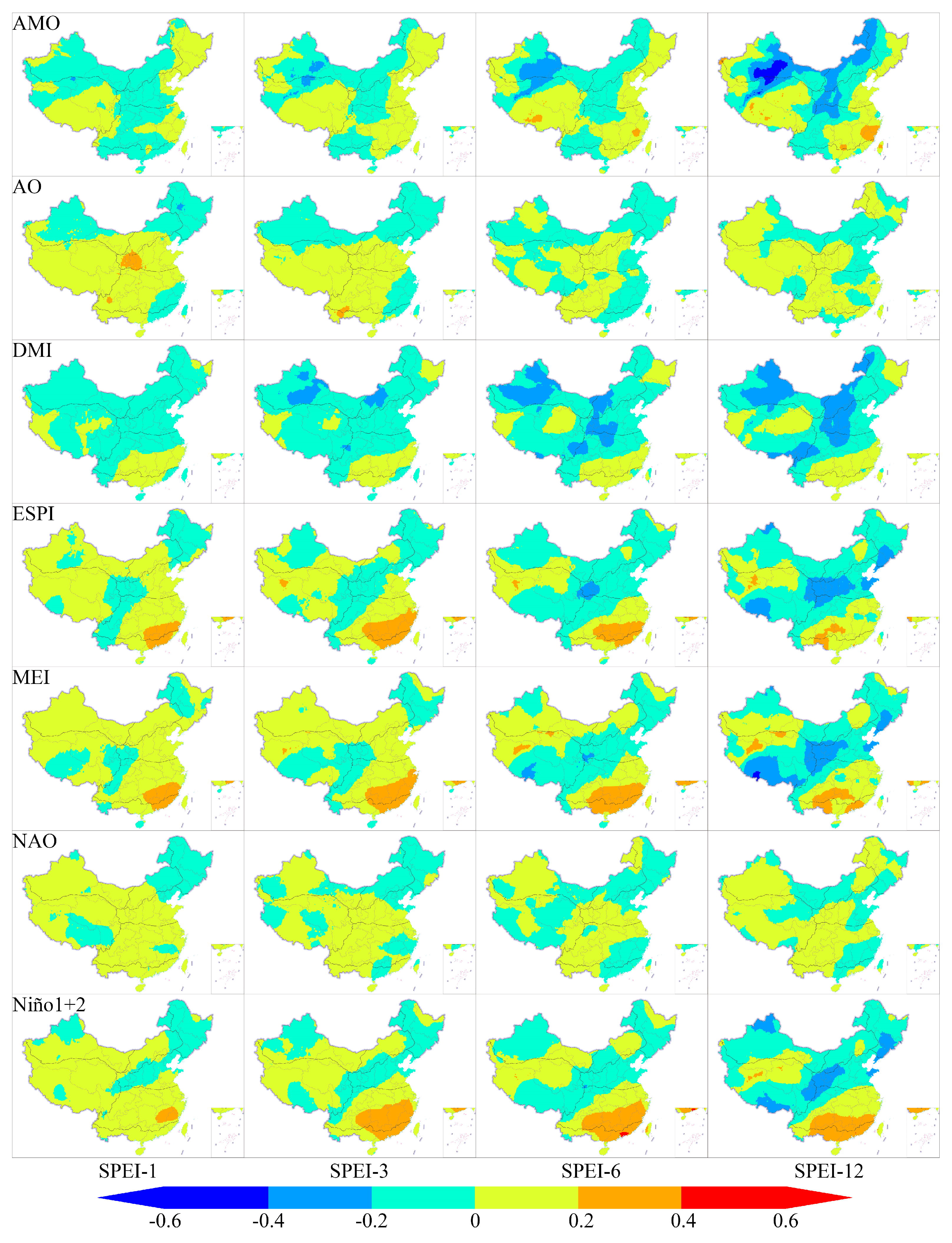
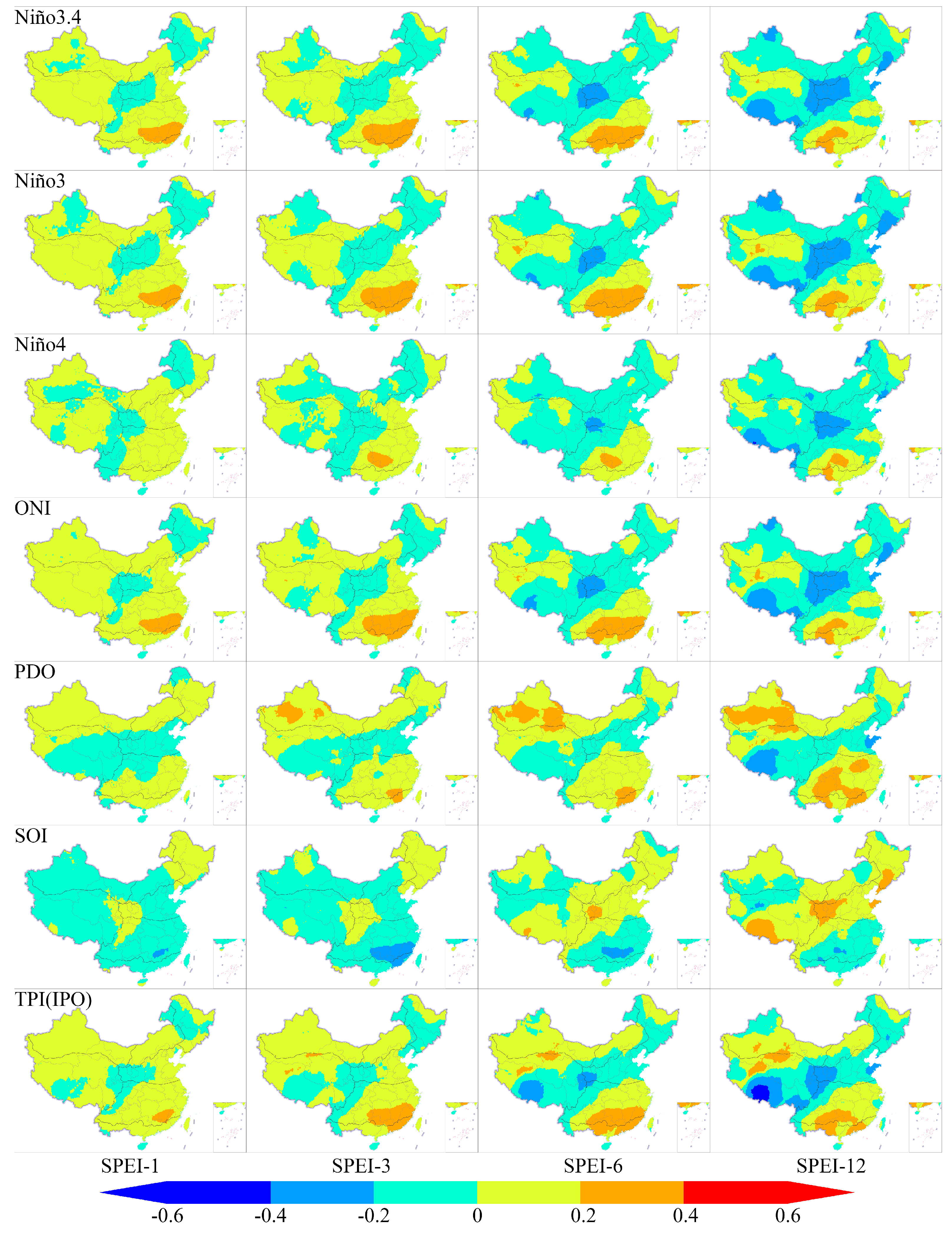
2.2.1. Pearson Correlation Analysis

The Pearson correlation coefficient quantifies linear dependence between paired variables, implemented to assess associations between SPEI series, atmospheric circulation indices, and lagged SPEI states. The coefficient is mathematically defined as:

$$r_{xy}={\displaystyle \frac{Cov\left(x,y\right)}{{\sigma }_x{\sigma }_y}}$$

(1)

where covariance $Cov\left(x,y\right)$ measures joint variability:

$$Cov\left(x,y\right)={\displaystyle \frac{\sum _{i=1}^N\left(x_i-\overline{x}\right)\left(y_i-\overline{y}\right)}{N-1}}$$

(2)

And standard deviations ${\sigma }_x, {\sigma }_y$ quantify dispersion:

$$\sigma =\sqrt{{\displaystyle \frac{1}{N}}{\sum }_{i=1}^N{\left(x_i-y_i\right)}^2}$$

(3)

Here, $x_i$ and $y_i$ denote paired observations, $\overline{x}$ and $\overline{y}$ their arithmetic means, and N the sample size.

2.2.2. XGBoost Architecture

XGBoost is a scalable ensemble algorithm based on the gradient-boosted decision tree framework [22], designed to improve predictive accuracy through an additive tree construction process. The model optimizes performance using a regularized objective function, which consists of a loss function measuring prediction error and a regularization term controlling model complexity. The objective function is given by:

$$\mathcal{L}\left(\mathsf{\Phi }\right)={\sum }_{i}l\left({\mathrm{ŷ}}_i-y_i\right)+{\sum }_k\mathsf{\Omega }\left(f_k\right)$$

(4)

where $l\left({\mathrm{ŷ}}_i-y_i\right)$ is a differentiable loss function (specifically the squared error loss function for regression tasks), ${\mathrm{ŷ}}_i$ denotes the predicted value for the i-th sample, and $y_i$ is the actual observed value for the iii-th sample. The term $f_k\left(x\right)$ represents the k-th regression tree in the ensemble, mapping input features x to predicted values, while $\mathsf{\Omega }\left(f_k\right)$ is the regularization term penalizing model complexity.

The regularization term is defined as:

$$\mathsf{\Omega }\left(f_k\right)=\gamma {{\rm T}}_k+{\displaystyle \frac{1}{2}}\lambda {\left|\right|{\omega }_k\left|\right|}^2$$

(5)

where ${{\rm T}}_k$ is the number of terminal nodes (leaves) in the k-th tree, and ${\omega }_k$ denotes the vector of leaf weights, which are the output values assigned to each leaf node. The hyperparameter $\gamma$ acts as a complexity penalty by discouraging excessive tree growth, while $\lambda$ controls the magnitude of leaf weights through L2 regularization, helping to prevent overfitting.

In the context of gradient-boosted decision trees, a leaf is the terminal node of a tree where final predictions are made. Each input sample is assigned to a specific leaf, and the corresponding weight ${\omega }_k$ serves as the predicted value. Trees with more leaves (${{\rm T}}_k$) allow for more detailed predictions but increase the risk of overfitting, necessitating proper regularization.

The XGBoost model was implemented using the R xgboost package (v4.0.4), with the following baseline hyperparameters: a learning rate of $\eta$ = 0.3, which controls the step size of each boosting iteration; a maximum tree depth of $d_{max}$ = 6, which limits tree growth to prevent excessive complexity; a subsample ratio of $\psi$ = 1.0, indicating that all training samples were used in each boosting round; and an initial L2 regularization coefficient of $\lambda$ = 0, meaning no additional penalty was applied to leaf weights in the baseline configuration.

To optimize model performance and prevent overfitting, the values of the regularization hyperparameters γ and λ were determined through grid search, systematically exploring a predefined range of parameter values. This approach ensured the selection of an optimal combination that balanced predictive accuracy and model complexity. Model performance was assessed using 100 bootstrap iterations, with evaluation metrics including the R², which quantifies how well the model explains variance in the observed data, and the RMSE, which measures the average magnitude of prediction errors.

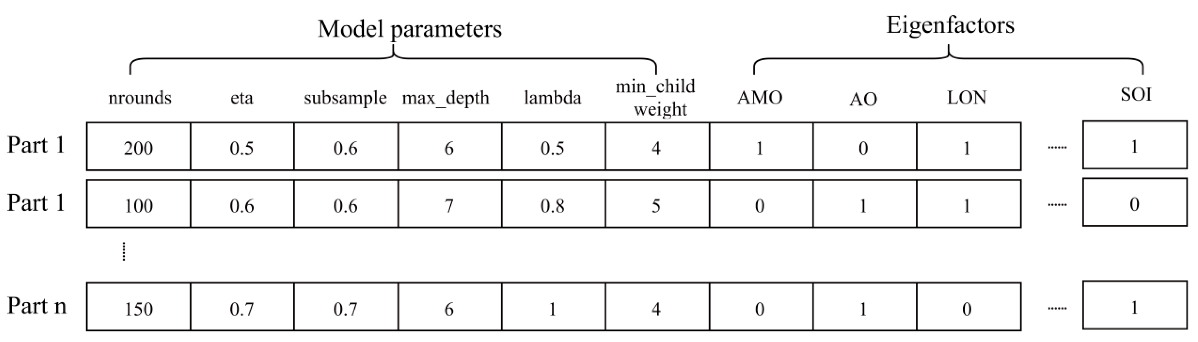
2.2.3. Hybrid Coding Particle Swarm Optimization

PSO is an optimization algorithm based on swarm intelligence, where particles (solution vectors) iteratively adjust their positions and velocities to search for the optimal solution. The velocity and position updates follow [23]:

$$\begin{array}{c}{v}_{id}^{t+1}={\omega v}_{id}^t+c_1{r}_1\left(p_{id}-x_{id}^t\right)+c_2{r}_2\left(g_d-x_{id}^t\right)\\ x_{id}^{t+1}=x_{id}^t+v_{id}^{t+1}\end{array}$$

Here, $v_{id}^t$ and $x_{id}^t$ represent the velocity and position of the i-th particle in the d-th dimension at iteration t, respectively. The inertia weight $\omega$ controls the trade-off between exploration and exploitation. The acceleration coefficients $c_1$ and $c_2$ determine the influence of the personal best position $p_{id}$ (the best solution found by the particle itself) and the global best position $g_d$ (the best solution found by the entire swarm). The random variables $r_1,r_2 ~\mathrm{U}\left(\mathrm{0,1}\right)$ introduce stochasticity to diversify the search process [24].

The CPSO framework coordinates continuous and discrete optimization through dual operational modes: (1) Continuous-space PSO optimizes six XGBoost hyperparameters—boosting iterations ($n_{estimators}\in \left[\mathrm{50,300}\right]$), learning rate (η∈[0.01,0.5]), maximum tree depth ($d_{max}\in \left\{3,\dots ,12\right\}$), and L2 regularization (λ∈[0,5]); (2) BPSO executes feature subspace selection across three predictive domains: atmospheric teleconnection indices, geospatial coordinates (longitude/latitude), and temporally lagged SPEI states (Leadtime-1, Leadtime-2, and Leadtime-3). This dual-mechanism architecture enables simultaneous hyperparameter tuning and physically constrained feature selection through parallelized swarm intelligence.

Through parallelized swarm intelligence, the CPSO-XGBoost system minimizes validation RMSE, identifying Pareto-optimal configurations that balance model complexity and predictive accuracy as demonstrated in Figure 2.

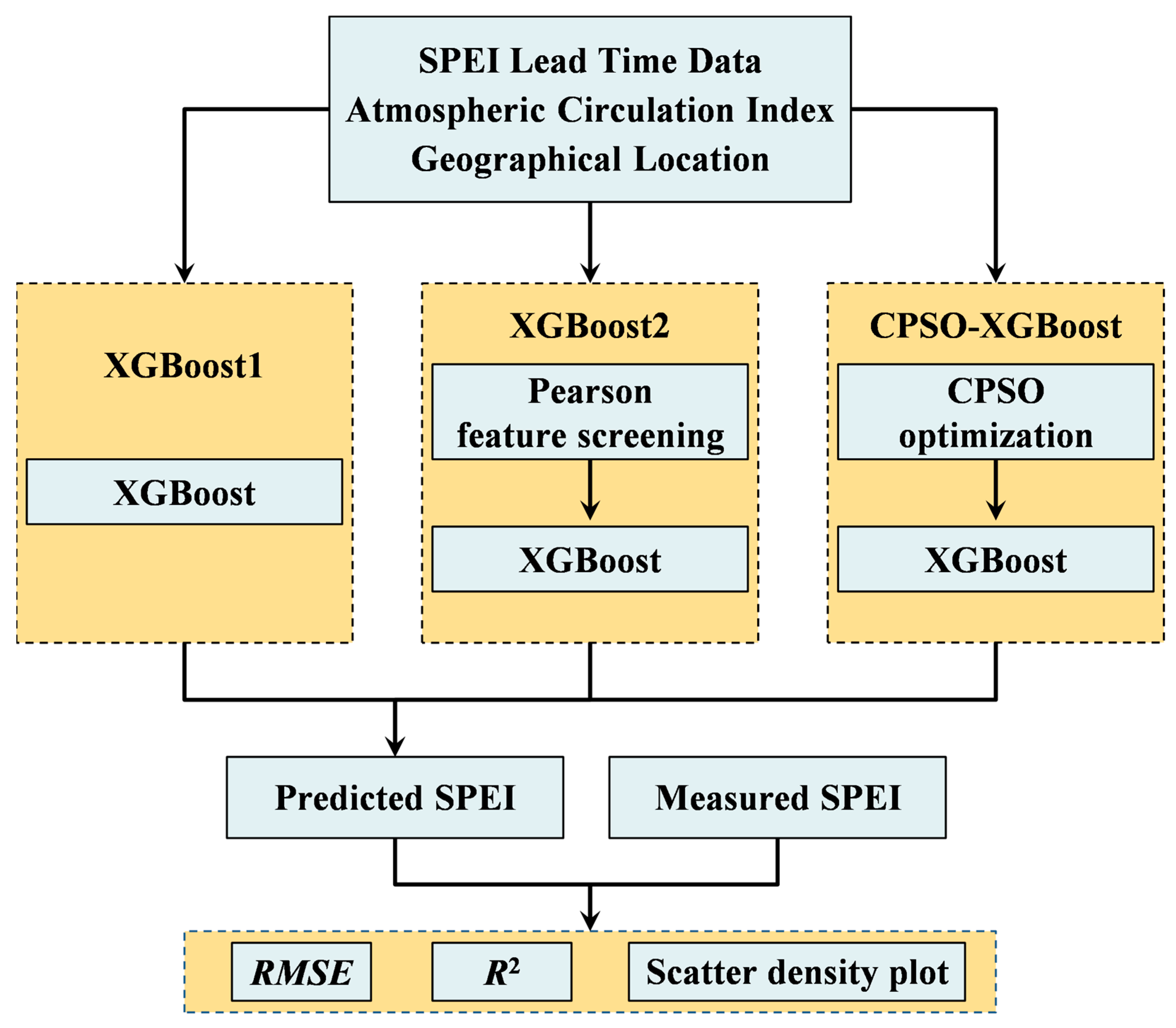
2.2.4. Predictive Model Architecture

Three distinct predictive architectures were implemented using atmospheric teleconnection indices, temporally lagged SPEI states, and geospatial determinants (longitude/latitude) as input covariates: (1) baseline XGBoost (XGBoost1) without optimization, (2) feature-optimized XGBoost (XGBoost2) with Pearson correlation-based selection, and (3) CPSO-XGBoost integrating hybrid parameter-feature optimization. The computational workflow—encompassing data preprocessing, feature engineering, model configuration, and optimization—is schematically represented in Figure 3.

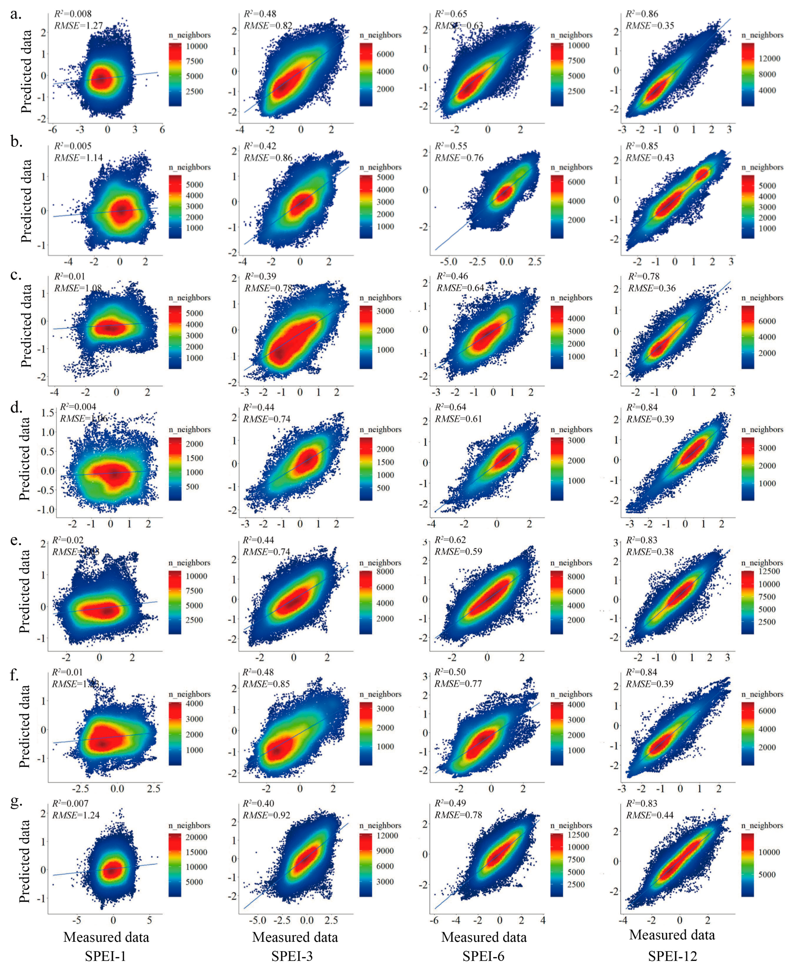
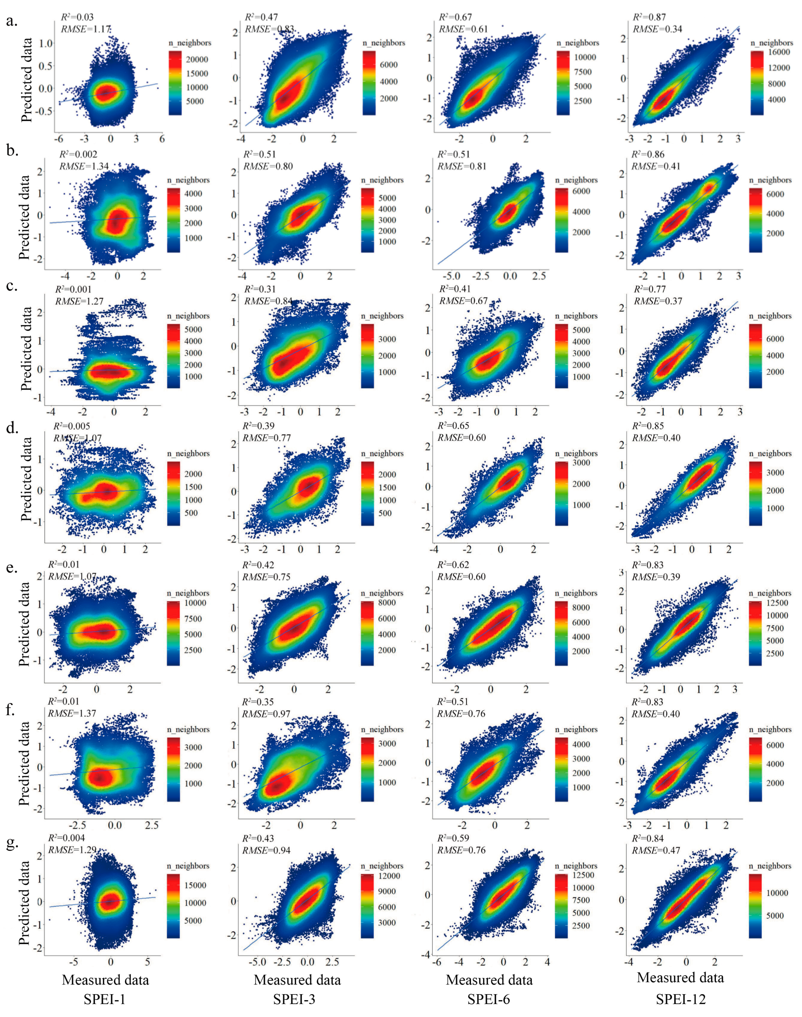
2.2.5. Predictive Model Evaluation

The observational dataset was partitioned into training (1979–2012) and testing (2013–2020) subsets to ensure temporal generalizability. Model predictive fidelity was quantified through two performance metrics:

$$RMSE=\sqrt{{\displaystyle \frac{1}{n}}{\sum }_{i=1}^n{\left(p\left(x_i\right)-y_i\right)}^2}$$

(6)

$$R^2=1-{\displaystyle \frac{\sum _{i=1}^n{\left(y_i-p\left(x_i\right)\right)}^2}{{\sum _{i=1}^n\left(y_i-{\overline{y}}_i\right)}^2}}$$

(7)

where $y_i$ denotes observed SPEI values, $p\left(x_i\right)$ model predictions, ${\overline{y}}_i$ the observational mean, and $n$ sample size. The R² approaches unity under perfect prediction–observation concordance, while RMSE asymptotically reduces to zero with increasing precision. These orthogonal metrics provided comprehensive assessment of model skill across the three architectures (XGBoost1, XGBoost2, CPSO-XGBoost).

3. Results

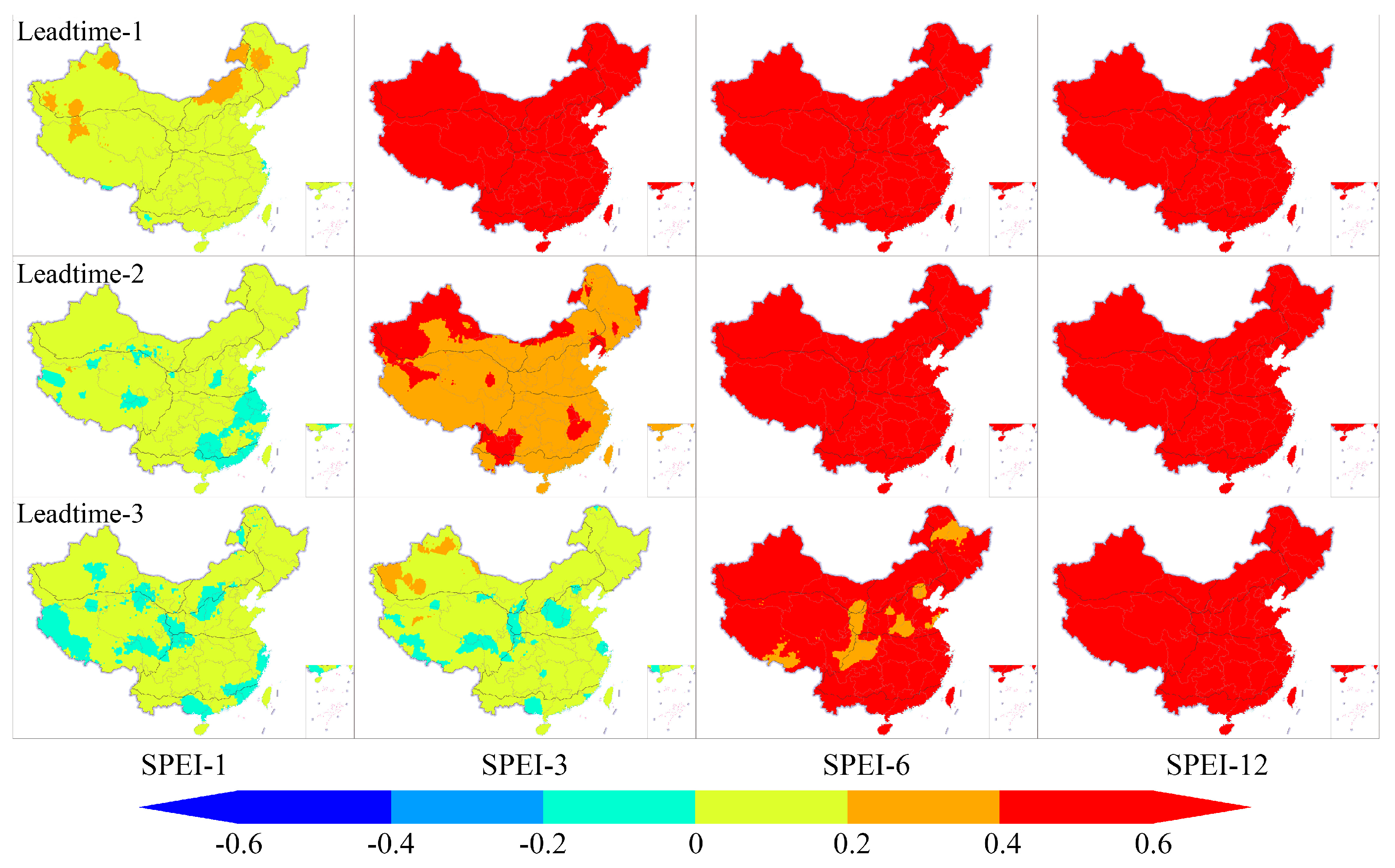
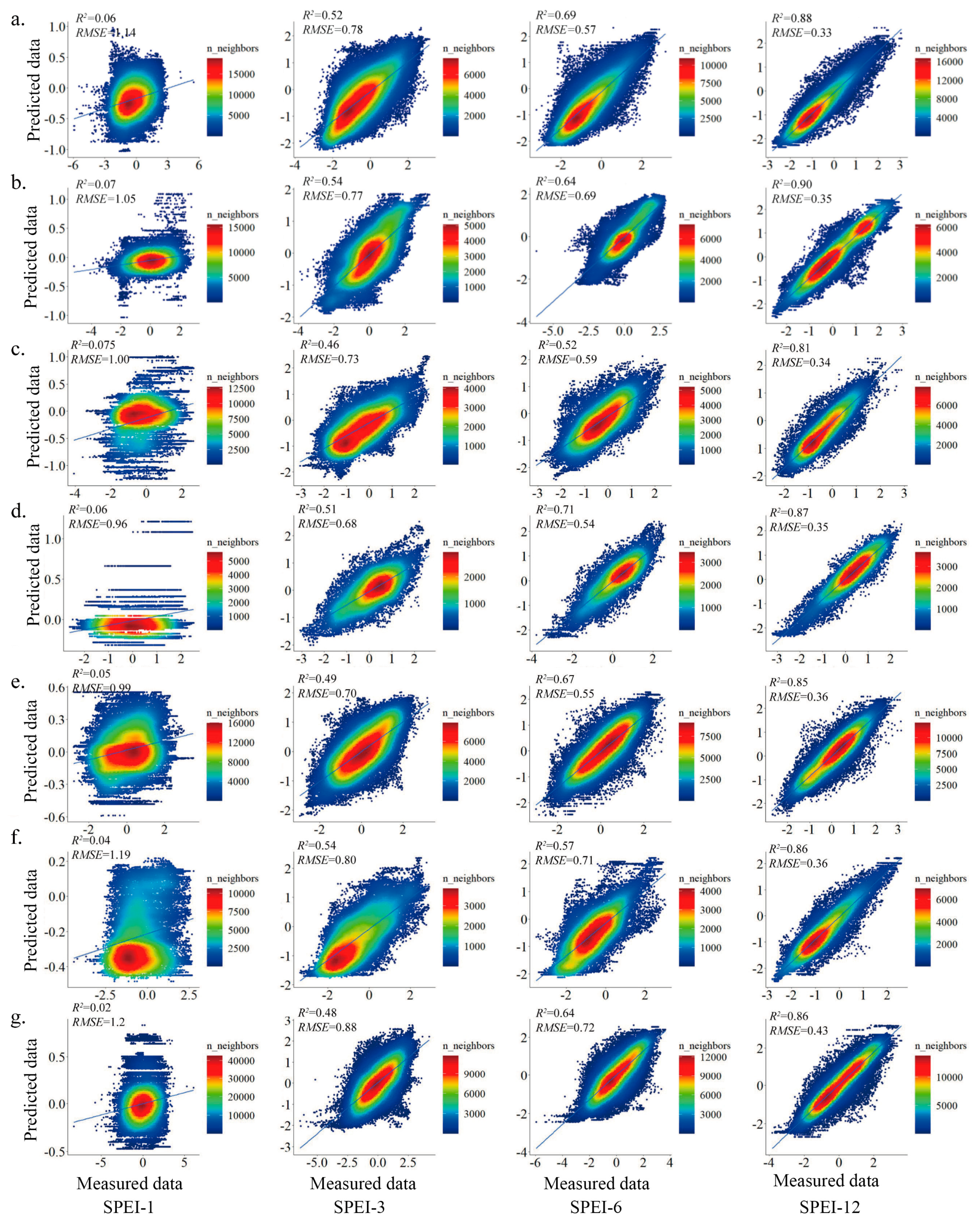
3.1. Short-Term Drought Prediction of SPEI in Mainland China Using the XGBoost1 Model

Figure 4 delineates the XGBoost1 model’s SPEI prediction efficacy across multi-temporal scales (SPEI-1–SPEI-12) in seven Chinese climatic regions, utilizing 19 covariates encompassing atmospheric oscillations, lagged SPEI states, and geospatial coordinates. The model exhibits superior predictive capability at extended temporal scales (SPEI-12: R² ≈ 0.83), where integration of long-term climate memory mitigates high-frequency climatic noise, thereby enhancing trend detection precision. This temporal scaling effect reduces RMSE by 38–47% compared to short-term forecasts (SPEI-1).

Regional analysis reveals pronounced hydroclimatic dependence: Humid zones (SCHTR, CSCHSR) demonstrate robust performance across all timescales (R² > 0.75), attributable to consistent precipitation regimes and stable land–atmosphere interactions. Conversely, arid/transitional regions (NDR, QTP, IMGR) exhibit limited short-term predictive skill (SPEI-1 R² < 0.45), reflecting complex moisture–atmosphere decoupling mechanisms. However, predictive fidelity improves markedly at longer scales (SPEI-12 R² > 0.71), as accumulated climatic signals override localized stochastic variability.

3.2. Short-Term Drought Prediction of SPEI in Mainland China Using the XGBoost2 Model

3.2.1. Extraction of Pearson Eigen Factors

Pearson correlation analysis revealed marked regional heterogeneity in the coupling between multi-scale SPEI series and 14 atmospheric circulation indices across China’s climatic zones (Figure 5, Figure 6 and Figure 7). In the NDR, SPEI-3 exhibited robust teleconnections with AMO, DMI, and PDO, while SPEI-12 demonstrated pan-basin synchronization with Niño3.4 and SOI. Transitional regions (IMGR, QTP) displayed short-term AO dominance (SPEI-1), evolving into mid-term DMI-driven moisture transport (SPEI-6) and long-term PDO-phase locking (SPEI-12). Humid monsoon zones (CSCHSR, SCHTR) showed intensified Indo-Pacific couplings, with SPEI-12 correlating strongly with MEI and Niño3.4. These patterns underscore scale-dependent atmosphere–ocean–land interactions modulated by regional hydroclimatic regimes.

Lead-time analysis (Figure 7) quantified memory effects across temporal scales: 1-month lags (Leadtime-1) dominated SPEI-1 predictions in high-altitude regions (QTP), while 3-month lags (Leadtime-3) governed SPEI-12 forecasts through cumulative teleconnections. The XGBoost2 architecture incorporated features exceeding geophysically meaningful thresholds (|r| > 0.2), prioritizing indices with dual statistical–climatological significance. Based on these findings, factors with an absolute correlation value exceeding 0.2 were selected as input features for the XGBoost2 model, considering their geographical significance. The detailed results of the feature selection process are presented in

Table 2. Input variables for the XGBoost2 model.

Time Scales	SPEI-1	SPEI-3	SPEI-6	SPEI-12
NDR	Latitude, Longitude, Leadtime-1	AMO, DMI, PDO, TPI(IPO), Longitude, Latitude, Leadtime-1, Leadtime-2, Leadtime-3	AMO, DMI, Niño3, Niño4, PDO, TPI(IPO), Longitude, Latitude, Leadtime-1, Leadtime-2, Leadtime-3	AMO, DMI, ESPI, MEI, Niño1+2, Niño3.4, Niño3, Niño4, ONI, PDO, SOI, TPI(IPO), Longitude, Latitude, Leadtime-1, Leadtime-2, Leadtime-3
IMGR	AO, Longitude, Latitude, Leadtime-1	DMI, Longitude, Latitude, Leadtime-1, Leadtime-2	DMI, Niño3.4, Niño3, Longitude, Latitude, Leadtime-1, Leadtime-2, Leadtime-3	AMO, DMI, ESPI, MEI, Niño1+2, Niño3.4, Niño3, Niño4, ONI, SOI, TPI(IPO), Longitude, Latitude, Leadtime-1, Leadtime-2, Leadtime-3
NHSTR	AO, Longitude, Latitude, Leadtime-1	Leadtime-1, Leadtime-2	SOI, Longitude, Latitude, Leadtime-1, Leadtime-2, Leadtime-3	AMO, DMI, ESPI, MEI, Niño1+2, Niño3.4, Niño3, Niño4, ONI, SOI, TPI(IPO), Longitude, Latitude, Leadtime-1, Leadtime-2, Leadtime-3
NHSTR	AO, Longitude, Latitude	DMI, Longitude, Latitude, Leadtime-1, Leadtime-2	DMI, ESPI, MEI, Niño1+2, Niño3.4, Niño3, Niño4, ONI, SOI, TPI(IPO), Longitude, Latitude, Leadtime-1, Leadtime-2, Leadtime-3	AMO, DMI, ESPI, MEI, Niño1+2, Niño3.4, Niño3, Niño4, ONI, PDO, SOI, TPI(IPO), Longitude, Latitude, Leadtime-1, Leadtime-2, Leadtime-3
QTP	AMO, AO, Longitude, Latitude, Leadtime-1, Leadtime-2	AMO, DMI, ESPI, MEI, Niño3, ONI, TPI(IPO), Longitude, Latitude, Leadtime-1, Leadtime-2, Leadtime-3	AMO, DMI, ESPI, MEI, Niño1+2, Niño3.4, Niño3, Niño4, ONI, PDO, SOI, TPI(IPO), Longitude, Latitude, Leadtime-1, Leadtime-2, Leadtime-3	AMO, DMI, ESPI, MEI, Niño1+2, Niño3.4, Niño3, Niño4, ONI, PDO, SOI, TPI(IPO), Longitude, Latitude, Leadtime-1, Leadtime-2, Leadtime-3
CSCHSR	AO, ESPI, MEI, Niño1+2, Niño3.4, Niño3, ONI, SOI, TPI(IPO), Longitude, Latitude	AO, DMI, ESPI, MEI, Niño1+2, Niño3.4, Niño3, Niño4, ONI, PDO, SOI, TPI(IPO), Longitude, Latitude, Leadtime-1, Leadtime-2	AMO, DMI, ESPI, MEI, Niño1+2, Niño3.4, Niño3, Niño4, ONI, PDO, SOI, TPI(IPO), Longitude, Latitude, Leadtime-1, Leadtime-2, Leadtime-3	AMO, DMI, ESPI, MEI, Niño1+2, Niño3.4, Niño3, Niño4, ONI, PDO, SOI, TPI(IPO), Longitude, Latitude, Leadtime-1, Leadtime-2, Leadtime-3
SCHTR	ESPI, MEI, Niño3.4, Niño3, ONI, TPI(IPO), Longitude, Latitude	AO, ESPI, MEI, Niño1+2, Niño3.4, Niño3, ONI, PDO, SOI, TPI(IPO), Longitude, Latitude, Leadtime-1, Leadtime-2	ESPI, MEI, Niño1+2, Niño3.4, Niño3, ONI, PDO, SOI, TPI(IPO), Longitude, Latitude, Leadtime-1, Leadtime-2, Leadtime-3	AMO, ESPI, MEI, Niño1+2, Niño3.4, Niño3, Niño4, ONI, PDO, SOI, TPI(IPO), Longitude, Latitude, Leadtime-1, Leadtime-2, Leadtime-3

Note: See Abbreviations List for definitions of all abbreviations.

.

3.2.2. Simulation Results of the Model

Figure 8 presents the performance of the XGBoost model, which uses input factors selected based on the Pearson correlation coefficient method, in simulating the SPEI at different time scales (SPEI-1, SPEI-3, SPEI-6, SPEI-12) across various regions. As the time scale increases, the model’s fitting performance improves significantly, as reflected by the increasing R² and decreasing RMSE values. This trend indicates that the input factors, selected based on correlation, effectively capture the influence of regional moisture dynamics and atmospheric circulation characteristics on the target variable, with particularly strong performance observed at longer time scales (e.g., SPEI-12).

Regional analysis reveals that the model performs best in humid and semi-humid regions, such as the NHSTR and the SCHTR. At the SPEI-12 time scale, the model achieves R² values exceeding 0.80, demonstrating high prediction accuracy and stability. In contrast, the model performs less effectively in the NDR and the NCHSWTR, especially at shorter time scales (SPEI-1 and SPEI-3), where R² values are lower, indicating greater uncertainty in these regions’ ecological–hydrological responses.

In the QTP, the model’s performance is intermediate compared to the other regions. At the SPEI-12 time scale, the fitting results are relatively strong (R² = 0.84, RMSE = 0.47). However, the scatter density plot shows some degree of dispersion between predicted and actual values. This uncertainty principally stems from the QTP’s unique geoclimatic configuration: intense surface heating (>120 W/m²) generates the Qinghai-Tibetan High, altering moisture transport via monsoon–anticyclone interactions; extreme elevational compression (3000–5000 m gradients within 50 km valleys) creates coexisting glaciers, wetlands, and arid zones that drive microclimate heterogeneity [25]. These coupled atmospheric–topographic dynamics produce subgrid-scale drought variations challenging for XGBoost to resolve with sparse station data.

3.3. Short-Term Drought Prediction of SPEI in Mainland China Using the CPSO-XGBoost Model

Figure 9 shows the SPEI prediction models based on the CPSO-XGBoost model for different regions and time scales (SPEI-1, SPEI-3, SPEI-6, SPEI-12). The results demonstrate that the time scale significantly impacts the model’s prediction performance. At longer time scales, such as SPEI-12, prediction accuracy improves markedly, with R² values generally exceeding 0.85 and RMSE decreasing to between 0.33 and 0.43. Conversely, at shorter time scales, such as SPEI-1, prediction performance is less accurate, with R² values ranging from 0.04 to 0.07 and higher RMSE values (greater than 1.0). These results suggest that longer time scales, reflecting cumulative climate effects, are more conducive to accurate predictions.

Regional climate conditions also have a substantial impact on model performance. In humid regions, such as the northeastern humid region, the model performs exceptionally well, especially at the SPEI-12 time scale, where R² reaches 0.90 and RMSE is around 0.35. In contrast, in arid and semi-arid regions, such as the NDR and IMGR, the model performs poorly at shorter time scales (with R² at 0.06 and RMSE of 1.19 for SPEI-1), but shows significant improvement at longer time scales (e.g., SPEI-12), with R² exceeding 0.85. The stable climate patterns and regular data in humid regions contribute to better prediction accuracy, whereas the high variability and complex climate conditions in arid regions challenge the model’s ability to capture their fluctuation patterns effectively.

The scatter density plots further illustrate the spatial distribution of prediction performance. In humid regions, data points are concentrated near the zero point, particularly at the longer SPEI-12 time scale, indicating a high degree of consistency between predicted and actual values, reflecting strong model fitting. In contrast, in arid and grassland regions, scatter points are more dispersed, especially in the extreme value range, with significant errors. This dispersion is likely due to the higher climate variability in these regions, which makes it difficult for the model to fully capture their complex fluctuations.

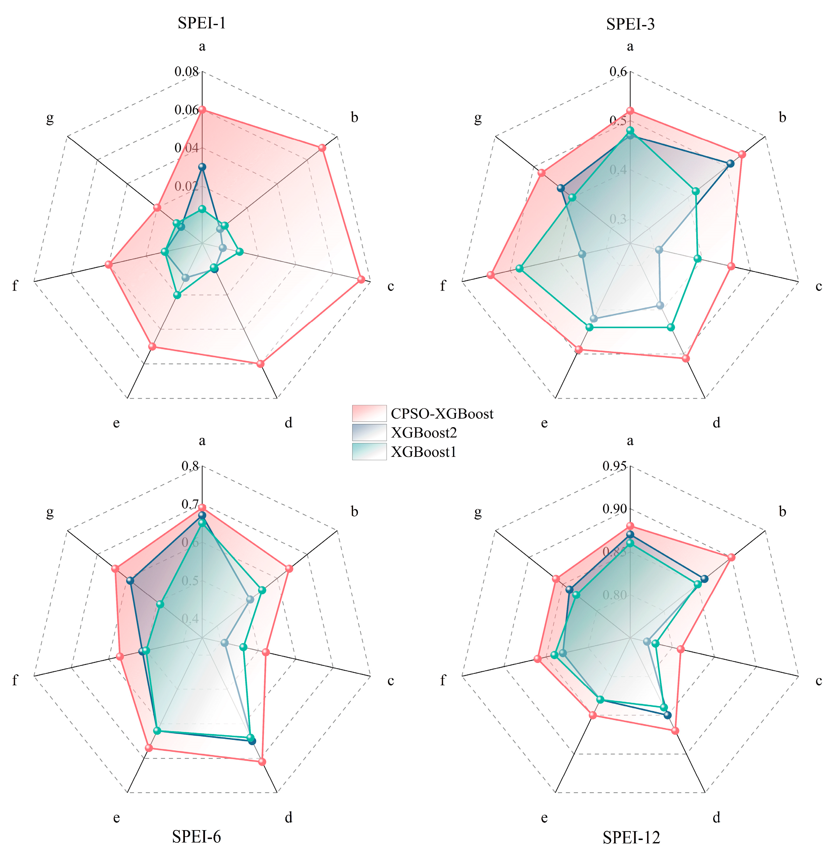
3.4. Comparative Analysis of Model Simulation Performance

The performance of all three models in predicting the SPEI at the SPEI-1 time scale is poor (Figure 10 and Figure 11), with RMSE values greater than 1 and R² values less than 0.1, indicating that the models have limited ability to predict the SPEI at shorter time scales. However, as the time scale increases to SPEI-3, SPEI-6, and SPEI-12, the models’ predictive performance improves significantly, with a notable reduction in RMSE and an increase in R², reflecting enhanced accuracy and stability at these longer time scales.

A comparison of the three models at different regional conditions and time scales shows that the CPSO-XGBoost model consistently outperforms both XGBoost1 and XGBoost2 models. For example, in the IMGR, the RMSE values for XGBoost1 at SPEI-3, SPEI-6, and SPEI-12 are 0.85, 0.77, and 0.39, with R² values of 0.48, 0.50, and 0.84. For XGBoost2, the RMSE values are 0.97, 0.76, and 0.40, with R² values of 0.35, 0.51, and 0.83. In contrast, the CPSO-XGBoost model achieves RMSE values of 0.80, 0.71, and 0.36, with R² values of 0.54, 0.57, and 0.86 at the same time scales. These results demonstrate that as the time scale increases, the prediction performance improves, and the CPSO-XGBoost model consistently provides the most accurate and stable predictions across all time scales.

4. Discussion

This study presents a comparative evaluation of three predictive models for the SPEI: XGBoost1, XGBoost2, and CPSO-XGBoost model. Among these, the CPSO-XGBoost model demonstrated significantly superior performance, highlighting its advantages in optimization mechanisms, predictive accuracy, and broad applicability.

The core strength of the CPSO-XGBoost model lies in its integrated optimization approach, combining PSO for parameter tuning and BPSO for feature selection. The PSO algorithm dynamically optimizes key model parameters, such as learning rate, tree depth, and regularization terms, through a global search process that avoids the limitations of traditional methods like grid search and random search [26,27]. Meanwhile, the BPSO algorithm identifies the most relevant feature subsets in high-dimensional data using binary encoding, effectively reducing redundancy and enhancing generalization [28]. This synergistic optimization ensures that the CPSO-XGBoost model not only captures complex nonlinear relationships but also remains computationally efficient, making it highly adaptable to diverse data characteristics and prediction tasks [29]. While atmospheric circulation indices (e.g., AMO, PDO, NAO) were critical predictors, their impacts on drought dynamics extend to soil moisture and vegetation feedback. For instance, prolonged negative phases of the PDO correlate with weakened East Asian monsoons, reducing rainfall in North China and depleting soil moisture reserves. This moisture deficit further suppresses vegetation productivity, intensifying land–atmosphere coupling and drought persistence—a feedback mechanism observed in the 2009–2011 Southwest China drought [30,31]. Future studies could explicitly integrate soil moisture–vegetation interactions to disentangle these cascading effects.

Previous studies confirm the effectiveness of PSO-based optimization in environmental modeling. A drought prediction study in Tamil Nadu, India, applied multi-objective optimization to improve classification in an imbalanced dataset, achieving a 45% precision improvement [32]. Another study in the same region used a weighted dataset approach with Gradient Boosting and Modified PSO, enhancing recall to 0.81 and identifying Mean Sea Level and CO₂ as key drought predictors [33]. Additionally, research on hydrological drought forecasting in Turkey’s Konya basin demonstrated the superiority of PSO-ANN models (R² = 0.468–0.931) over conventional methods [34]. These findings collectively validate the effectiveness of PSO-enhanced models for improving drought and hydrometeorological predictions, further supporting the advantages of the CPSO-XGBoost model in this study. To bridge the gap between atmospheric drivers and land–surface processes, future iterations of the CPSO-XGBoost framework could integrate high-resolution soil moisture data and real-time evapotranspiration estimates, enabling direct quantification of soil water balance dynamics and their coupling with atmospheric teleconnections [35,36]. Incorporating these variables would enhance the model’s capacity to resolve localized drought triggers, particularly in regions with complex land-use transitions.

The simulation results underscore the superior predictive performance of the CPSO-XGBoost model, particularly at larger time scales. For the SPEI-12, the CPSO-XGBoost model achieved an R² of 0.86, surpassing both the XGBoost2 model (R² = 0.83) and the XGBoost1 model (R² = 0.84). Additionally, its lower RMSE indicates a closer alignment between predicted and actual values, demonstrating the model’s ability to accurately capture SPEI dynamics. Notably, the CPSO-XGBoost model exhibited enhanced performance as time scales increased, further showcasing its capability to model complex feature–target relationships [37]. Short-term drought forecasting (SPEI-1) remains challenging due to the high stochasticity of meteorological variables (e.g., localized precipitation extremes) and limited persistence in soil moisture anomalies. In arid regions like the NDR, rapid evapotranspiration responses to temperature fluctuations amplify prediction uncertainties, as soil moisture deficits are quickly exacerbated by high atmospheric demand [38]. These challenges are compounded by the sparse observational networks in remote areas, limiting real-time data assimilation for sub-seasonal forecasts. In contrast, the XGBoost2 model, constrained by its reliance on linear correlations for feature selection, underperformed in capturing nonlinear interactions [39]. Similarly, the XGBoost1 model, without optimization, suffered from feature redundancy and suboptimal parameter settings, resulting in less robust predictions.

Beyond predictive accuracy, the CPSO-XGBoost model also excels in computational efficiency and practical applicability. By leveraging BPSO for feature selection, the model reduces computational complexity without compromising performance [40], making it particularly effective for high-dimensional datasets. Simultaneously, the PSO-optimized parameters enhance convergence speed and robustness [41], ensuring stable predictions across varying temporal and spatial contexts. To contextualize the model’s performance, we compared the predicted SPEI anomalies with documented historical droughts in China. For example, during the 2009–2011 Southwest China drought (SPEI-12 < −2.0), the region exhibited persistent negative SPEI-12 values in observational records [42], which aligns with the model’s capability to capture long-term drought persistence. Similarly, the 2014 North China Plain water crisis corresponded to SPEI-6 values below −1.5 in both predictions and station data [43]. While these comparisons are qualitative due to the lack of ground-truth validation in our training data, they suggest the model’s potential to replicate known drought patterns. Recent advances in drought quantification, such as the NDI that integrates soil–vegetation–atmosphere interactions [44,45], offer promising avenues for enhancing short-term forecasting. While our operational framework currently prioritizes SPEI for its compatibility with China Meteorological Administration protocols, the modular architecture of CPSO-XGBoost could readily assimilate NDI’s microwave-based soil moisture inputs—a critical advantage for arid regions where SPEI-1 performance remains suboptimal (R² < 0.35 in NDR). In contrast, the XGBoost1 model’s use of all features and default parameters leads to higher computational demands and susceptibility to overfitting [46]. While the XGBoost2 model alleviates some redundancy, its linear feature selection limits its efficiency and accuracy compared to the CPSO-XGBoost model.

In summary, the CPSO-XGBoost model represents a comprehensive advancement in SPEI prediction by integrating parameter optimization and feature selection. Its robust performance across metrics and time scales establishes it as a reliable and efficient tool for drought monitoring and prediction in China. Future work should prioritize two directions: (1) integrating land-surface hydrology variables (e.g., soil moisture, groundwater levels) with historical drought impact records (e.g., crop yield losses, reservoir depletion) to enable mechanistic validation; (2) assimilating real-time satellite precipitation products to enhance short-term forecasting in data-sparse regions; and (3) a comparative paradigm should be developed to systematically evaluate emerging drought indices against SPEI under shared climatic forcing, with a particular focus on their complementary strengths in detecting rapid-onset agricultural droughts versus long-term meteorological extremes. The CPSO-XGBoost model offers valuable insights for water resource management, agricultural drought risk mitigation, and early warning systems. Furthermore, it sets a precedent for leveraging machine learning in addressing meteorological disasters, paving the way for innovative applications in environmental science and beyond.

5. Conclusions

This study systematically evaluated three short-term drought prediction models, XGBoost1, XGBoost2, and CPSO-XGBoost, with the aim of improving the prediction accuracy of the SPEI across multiple timescales in China. The findings reveal that while all models exhibit lower performance at short time scales (e.g., SPEI-1) with relatively large prediction errors, their performance improves significantly at longer time scales (e.g., SPEI-12). Among the models, the CPSO-XGBoost model demonstrates the most substantial improvement, achieving an R² exceeding 0.85 and a markedly reduced RMSE, making it the most accurate and reliable model in this study. Additionally, the CPSO-XGBoost model performs exceptionally well in long-term drought prediction for humid regions such as South China, achieving an R² close to 0.90 and maintaining a low RMSE. In contrast, while the model struggles at short time scales in arid regions and areas with complex terrain, such as the NDR and the QTP, its performance improves notably as the time scale increases, reflecting its adaptability to diverse environmental conditions and varying drought characteristics.

The superior performance of the CPSO-XGBoost model can be attributed to its robust capacity for modeling complex nonlinear relationships, driven by the synergistic effects of its feature selection and parameter optimization mechanisms. By employing BPSO for selecting highly relevant features and PSO for fine-tuning model parameters, the CPSO-XGBoost achieves a comprehensive balance between computational efficiency and predictive accuracy. This not only reduces feature redundancy and improves generalization ability but also ensures the model’s stability and adaptability across different time scales and regional contexts.

In conclusion, the CPSO-XGBoost model offers an efficient and accurate approach to drought prediction, with significant scientific and practical implications for water resource management, agricultural drought risk early warning, and meteorological disaster response under the pressures of climate change. By leveraging advanced optimization techniques, this model provides a robust framework for enhancing drought prediction capabilities and sets a strong foundation for future innovations in machine learning-based environmental modeling.

References

1. Wang, X.Y.; Li, J.; Xing, L.T. Comparative agricultural drought monitoring based on three machine learning methods. Arid Zone Res. 2022, 39, 322–332. [Google Scholar]
2. Wang, Y.; Wang, L.; Lu, X.; Zhang, J.; Wang, Z.; Sha, S.; Hu, D.; Yang, Y.; Yan, P.; Li, Y. Analysis of the characteristics and causes of drought in China in the first half of 2023. J. Arid Meteorol. 2023, 41, 884. [Google Scholar]
3. Zhang, R.; Chen, Z.Y.; Xu, L.J.; Ou, C.Q. Meteorological drought forecasting based on a statistical model with machine learning techniques in Shaanxi province, China. Sci. Total Environ. 2019, 665, 338–346. [Google Scholar] [CrossRef] [PubMed]
4. Zhang, Q.; Yao, Y.; Li, Y.; Huang, J.; Ma, Z.; Wang, Z.; Wang, S.; Wang, Y.; Zhang, Y. Progress and prospect on the study of causes and variation regularity of droughts in China. Acta Meteorol. Sin. 2020, 78, 500–521. [Google Scholar] [CrossRef]
5. Achite, M.; Jehanzaib, M.; Elshaboury, N.; Kim, T.W. Evaluation of Machine Learning Techniques for Hydrological Drought Modeling: A Case Study of the Wadi Ouahrane Basin in Algeria. Water 2022, 14, 431. [Google Scholar] [CrossRef]
6. Vicente-Serrano, S.M.; Beguería, S.; López-Moreno, J.I. A multiscalar drought index sensitive to global warming: The standardized precipitation evapotranspiration index. J. Clim. 2010, 23, 1696–1718. [Google Scholar] [CrossRef]
7. Chen, T.; Guestrin, C.X. Xgboost: A scalable tree boosting system. In Proceedings of the 22nd ACM SIGKDD International Conference on Knowledge Discovery and Data Mining, San Francisco, CA, USA, 13–17 August 2016; pp. 785–794. [Google Scholar]
8. Milevski, I.; Aleksova, B.; Lukić, T.; Dragićević, S.; Valjarević, A. Multi-Hazard Modeling of Erosion and Landslide Susceptibility at the National Scale in the Case of North Macedonia. Open Geosci. 2024, 16, 20220718. [Google Scholar] [CrossRef]
9. Valjarević, A.; Morar, C.; Brasanac-Bosanac, L.; Cirkovic-Mitrovic, T.; Djekic, T.; Mihajlović, M.; Kaplan, G. Sustainable Land Use in Moldova: GIS & Remote Sensing of Forests and Crops. Land Use Policy 2025, 152, 107515. [Google Scholar]
10. Bergstra, J.; Bengio, Y. Random search for hyper-parameter optimization. J. Mach. Learn. Res. 2012, 13, 281–305. [Google Scholar]
11. Freitas, D.; Lopes, L.G.; Morgado-Dias, F. Particle swarm optimisation: A historical review up to the current developments. Entropy 2020, 22, 362. [Google Scholar] [CrossRef]
12. Papazoglou, G.; Biskas, P. Review and comparison of genetic algorithm and particle swarm optimization in the optimal power flow problem. Energies 2023, 16, 1152. [Google Scholar] [CrossRef]
13. Yu, J.; Zheng, W.; Xu, L.; Zhangzhong, L.; Zhang, G.; Shan, F. A PSO-XGBoost model for estimating daily reference evapotranspiration in the solar greenhouse. Intell. Autom. Soft Comput. 2020, 26, 989–1003. [Google Scholar] [CrossRef]
14. Jia, H.J.; Li, X.H.; Wang, L.; Xue, Y.; Lin, H. Remote sensing drought monitoring and assessment in southwestern China based on machine learning. Plateau Meteorol. 2022, 41, 1572–1582. [Google Scholar]
15. Kumar, S.; Tian, D. Causal Discovery Analysis Reveals Global Sources of Predictability for Regional Flash Droughts. Water Resour. Res. 2024, 60, e2024WR038391. [Google Scholar] [CrossRef]
16. Liu, C.; Zhang, X.; Nguyen, T.T.; Liu, J.; Wu, T.; Lee, E.; Tu, X.M. Partial least squares regression and principal component analysis: Similarity and differences between two popular variable reduction approaches. Gen. Psychiatry 2022, 35, e100662. [Google Scholar] [CrossRef]
17. Jiang, J.; Atkinson, P.M.; Chen, C.; Cao, Q.; Tian, Y.; Zhu, Y.; Liu, X.; Cao, W. Combining UAV and Sentinel-2 satellite multi-spectral images to diagnose crop growth and N status in winter wheat at the county scale. Field Crop. Res. 2023, 294, 108860. [Google Scholar] [CrossRef]
18. Joshi, A.; Pradhan, B.; Chakraborty, S.; Behera, M.D. Winter wheat yield prediction in the conterminous United States using solar-induced chlorophyll fluorescence data and XGBoost and random forest algorithm. Ecol. Inform. 2023, 77, 102194. [Google Scholar] [CrossRef]
19. Yang, J.; Tian, Y.; Wu, C.H. Air quality prediction and ranking assessment based on bootstrap-XGBoost algorithm and ordinal classification models. Atmosphere 2024, 15, 925. [Google Scholar] [CrossRef]
20. Lyu, Y.; Yong, B. A Novel Double Machine Learning Strategy for Producing High-Precision Multi-Source Merging Precipitation Estimates over the Tibetan Plateau. Water Resour. Res. 2024, 60, e2023WR035643. [Google Scholar] [CrossRef]
21. Dong, J.; Zeng, W.; Wu, L.; Huang, J.; Gaiser, T.; Srivastava, A.K. Enhancing short-term forecasting of daily precipitation using numerical weather prediction bias correcting with XGBoost in different regions of China. Eng. Appl. Artif. Intell. 2023, 117, 105579. [Google Scholar] [CrossRef]
22. Ma, M.; Zhao, G.; He, B.; Li, Q.; Dong, H.; Wang, S.; Wang, Z. XGBoost-based method for flash flood risk assessment. J. Hydrol. 2021, 598, 126382. [Google Scholar] [CrossRef]
23. Eberhart, R.; Kennedy, J. A new optimizer using particle swarm theory. In Proceedings of the Sixth International Symposium on Micro Machine and Human Science (MHS’95), Nagoya, Japan, 4–6 October 1995; IEEE: New York, NY, USA, 1995; pp. 39–43. [Google Scholar]
24. Xiujia, C.; Guanghua, Y.; Jian, G.; Ningning, M.; Zihao, W. Application of WNN-PSO model in drought prediction at crop growth stages: A case study of spring maize in semi-arid regions of northern China. Comput. Electron. Agric. 2022, 199, 107155. [Google Scholar] [CrossRef]
25. Wang, Z.; Cui, G.; Liu, X.; Zheng, K.; Lu, Z.; Li, H.; Wang, G.; An, Z. Greening of the Qinghai–Tibet Plateau and Its Response to Climate Variations along Elevation Gradients. Remote Sens. 2021, 13, 3712. [Google Scholar] [CrossRef]
26. Qolomany, B.; Maabreh, M.; Al-Fuqaha, A.; Gupta, A.; Benhaddou, D. Parameters optimization of deep learning models using particle swarm optimization. In Proceedings of the 2017 13th International Wireless Communications and Mobile Computing Conference (IWCMC), Valencia, Spain, 26–30 June 2017; IEEE: New York, NY, USA, 2017; pp. 1285–1290. [Google Scholar]
27. Fan, Y.; Zhang, Y.; Guo, B.; Luo, X.; Peng, Q.; Jin, Z. A hybrid sparrow search algorithm of the hyperparameter optimization in deep learning. Mathematics 2022, 10, 3019. [Google Scholar] [CrossRef]
28. Li, A.D.; Xue, B.; Zhang, M. Improved binary particle swarm optimization for feature selection with new initialization and search space reduction strategies. Appl. Soft Comput. 2021, 106, 107302. [Google Scholar]
29. Zhou, G.; Gao, J.; Zuo, D.; Li, J.; Li, R. MSXFGP: Combining improved sparrow search algorithm with XGBoost for enhanced genomic prediction. BMC Bioinform. 2023, 24, 384. [Google Scholar] [CrossRef]
30. Wang, Z.; Chen, W.; Piao, J.; Cai, Q.; Chen, S.; Xue, X.; Ma, T. Synergistic Effects of High Atmospheric and Soil Dryness on Record-Breaking Decreases in Vegetation Productivity over Southwest China in 2023. NPJ Clim. Atmos. Sci. 2025, 8, 6. [Google Scholar]
31. Jiang, L.; Chen, Y.D.; Li, J.; Liu, C. Amplification of Soil Moisture Deficit and High Temperature in a Drought-Heatwave Co-Occurrence in Southwestern China. Nat. Hazards 2022, 111, 641–660. [Google Scholar] [CrossRef]
32. Sundararajan, K.; Srinivasan, K. A Synergistic Optimization Algorithm with Attribute and Instance Weighting Approach for Effective Drought Prediction in Tamil Nadu. Sustainability 2024, 16, 2936. [Google Scholar] [CrossRef]
33. Sundararajan, K.; Srinivasan, K.; Kaliappan, J. Improving Meteorological Drought Prediction in Tamil Nadu through Weighted Dataset Construction and Multi-Objective Optimization. IEEE Access 2024, 12, 96878–96892. [Google Scholar]
34. Katipoğlu, O.M.; Ertugay, N.; Elshaboury, N.; Aktürk, G.; Kartal, V.; Pande, C.B. A Novel Metaheuristic Optimization and Soft Computing Techniques for Improved Hydrological Drought Forecasting. Phys. Chem. Earth A/B/C 2024, 135, 103646. [Google Scholar]
35. Zhang, C.; Long, D.; Zhang, Y.; Anderson, M.C.; Kustas, W.P.; Yang, Y. A Decadal (2008–2017) Daily Evapotranspiration Data Set of 1 km Spatial Resolution and Spatial Completeness across the North China Plain Using TSEB and Data Fusion. Remote Sens. Environ. 2021, 262, 112519. [Google Scholar]
36. Ghilain, N. Continental Scale Monitoring of Subdaily and Daily Evapotranspiration Enhanced by the Assimilation of Surface Soil Moisture Derived from Thermal Infrared Geostationary Data. In Satellite Soil Moisture Retrieval; Elsevier: Amsterdam, The Netherlands, 2016; pp. 309–332. [Google Scholar]
37. Wang, C.C.; Kuo, P.H.; Chen, G.Y. Machine learning prediction of turning precision using optimized XGBoost model. Appl. Sci. 2022, 12, 7739. [Google Scholar] [CrossRef]
38. He, B.; Wang, H.; Guo, L.; Liu, J. Global Analysis of Ecosystem Evapotranspiration Response to Precipitation Deficits. J. Geophys. Res. Atmos. 2017, 122, 13–308. [Google Scholar]
39. Ratnasingam, S.; Muñoz-Lopez, J. Distance correlation-based feature selection in random forest. Entropy 2023, 25, 1250. [Google Scholar] [CrossRef]
40. Han, D.; Li, H.; Fu, X. Reflective distributed denial of service detection: A novel model utilizing binary particle swarm optimization—Simulated annealing for feature selection and gray wolf optimization-optimized LightGBM algorithm. Sensors 2024, 24, 6179. [Google Scholar] [CrossRef]
41. Lavate, S.; Joshi, A.A.; Shinde, T.S. Enhancing the convergence speed and accuracy of particle swarm optimizers through adaptive learning. In Proceedings of the 2022 International Conference on Emerging Smart Computing and Informatics (ESCI), Pune, India, 4–5 March 2022; IEEE: New York, NY, USA, 2022; pp. 1–6. [Google Scholar]
42. Wang, W.; Zhu, Y.; Xu, R.; Liu, J. Drought Severity Change in China during 1961–2012 Indicated by SPI and SPEI. Nat. Hazards 2015, 75, 2437–2451. [Google Scholar]
43. Chen, X.; Mo, X.; Zhang, Y.; Sun, Z.; Liu, Y.; Hu, S.; Liu, S. Drought Detection and Assessment with Solar-Induced Chlorophyll Fluorescence in Summer Maize Growth Period over North China Plain. Ecol. Indic. 2019, 104, 347–356. [Google Scholar]
44. Bonacci, O.; Žaknić-Ćatović, A.; Roje-Bonacci, T. Prominent Increase in Air Temperatures on Two Small Mediterranean Islands, Lastovo and Lošinj, Since 1998 and Its Effect on the Frequency of Extreme Droughts. Water 2024, 16, 3175. [Google Scholar] [CrossRef]
45. Bonacci, O.; Bonacci, D.; Roje-Bonacci, T.; Vrsalović, A. Proposal of a New Method for Drought Analysis. J. Hydrol. Hydromech. 2023, 71, 100–110. [Google Scholar]
46. Xia, Y.; Jiang, S.; Meng, L.; Ju, X. XGBoost-B-GHM: An ensemble model with feature selection and GHM loss function optimization for credit scoring. Systems 2024, 12, 254. [Google Scholar] [CrossRef]
Figure 1. Regional division of mainland China into seven major areas. See Abbreviations List for definitions of all abbreviations.
Atmosphere 16 00419 g001
Figure 2. Distribution of coding strategies in the CPSO-XGBoost model.
Atmosphere 16 00419 g002
Figure 3. Framework of the model-building process.
Atmosphere 16 00419 g003
Figure 4. Scatter density plot of the XGBoost1 model’s simulation of SPEI at four scales across seven major regions of mainland China. (a). NDR; (b). NHSTR; (c). NCHSWTR; (d). SCHTR; (e). CSCHSR; (f). IMGR; (g). QTP. See Abbreviations List for definitions of all abbreviations.
Atmosphere 16 00419 g004
Figure 5. Spatial correlation between SPEI and atmospheric circulation indices (AMO−Niño1+2). The parameter name in the upper left corner corresponds to each subplot. See Abbreviations List for definitions of all abbreviations.
Atmosphere 16 00419 g005
Figure 6. Spatial correlation between SPEI and atmospheric circulation indices (Niño3.4− TPI(IPO)). The parameter name in the upper left corner corresponds to each subplot. See Abbreviations List for definitions of all abbreviations.
Atmosphere 16 00419 g006
Figure 7. Spatial correlation between SPEI and lagged SPEI values. See Abbreviations List for definitions of all abbreviations.
Atmosphere 16 00419 g007
Figure 8. Scatter density plot of the XGBoost2 model’s simulation of SPEI at four timescales across seven major regions of China. (a). NDR; (b). NHSTR; (c). NCHSWTR; (d). SCHTR; (e). CSCHSR; (f). IMGR; (g). QTP. See Abbreviations List for definitions of all abbreviations.
Atmosphere 16 00419 g008
Figure 9. Scatter density plot of the CPSO-XGBoost model’s simulation of SPEI at four timescales across seven major regions of China. (a). NDR; (b). NHSTR; (c). NCHSWTR; (d). SCHTR; (e). CSCHSR; (f). IMGR; (g). QTP. See Abbreviations List for definitions of all abbreviations.
Atmosphere 16 00419 g009
Figure 10. Comparison of R2 values for different models in simulating SPEI at multiple timescales across seven major regions of China. (a). NDR; (b). NHSTR; (c). NCHSWTR; (d). SCHTR; (e). CSCHSR; (f). IMGR; (g). QTP. See Abbreviations List for definitions of all abbreviations.
Atmosphere 16 00419 g010
Figure 11. Comparison of RMSE values for different models in simulating SPEI at multiple timescales across seven major regions of China. (a). NDR; (b). NHSTR; (c). NCHSWTR; (d). SCHTR; (e). CSCHSR; (f). IMGR; (g). QTP. See Abbreviations List for definitions of all abbreviations.
Atmosphere 16 00419 g011