Atmospheric Energetics of Three Contrasting West African Monsoon Seasons as Simulated by a Regional Climate Model

Abstract

The West African atmospheric energy budget is assessed for the first time across three contrasting monsoon seasons (dry, wet, and moderate) using the latest version of the Canadian Regional Climate Model (CRCM6/GEM5). The model is driven by ERA5 reanalysis from the European Centre for Medium-Range Weather Forecasts (ECMWF). A formalism appropriate for regional climate energetics is employed to quantify the primary physical processes occurring during the West African Monsoon, with the aim of highlighting those that exhibit significant inter-seasonal variability. The atmospheric energy path shows that the time-mean available enthalpy (A_M) reservoir, reflecting high surface temperatures and a lapse rate characteristic of a dry atmosphere, dominates other energy reservoirs. A_M is converted into the time-mean kinetic energy (K_M) and the time-variability available enthalpy (A_E) reservoirs, which are converted into a time-variability kinetic energy reservoir (K_E) through barotropic and baroclinic processes. A_E is the lowest energy reservoir, confirming smaller temperature variations in the tropics compared to higher latitudes. Kinetic energy reservoirs K_M and K_E have the same order of magnitude, suggesting that mean flow is as important as eddy activities during the season. The atmospheric energy cycle computed for three contrasting rainy seasons shows that time-variability energy reservoirs (A_E and K_E) and main terms acting upon them, are proportional to the rainfall activity, being higher (lower) during rainy (dry) years. It also reveals that, while C_A (conversion from A_M to A_E) and the generation term G_E feed wave’s development, the frictional term D_E counteracts the generation of K_E to dampen the creation of transient eddies. These findings suggest that the atmospheric energetic formalism could be applied on West African seasonal forecasts and future climate simulations to implement adaptation strategies.

1. Introduction

During the boreal summer, the northward shift in monsoon flow brings a huge amount of humidity over the West African hot continental surface, producing the rainy period of the year in the southern belt of the Sahara Desert, the Sahel. This phenomenon, known as the West African Monsoon (WAM), is the most important feature of the West African climate. The WAM exhibits large interannual variability in terms of rainfall occurrence, the amount, and geographic distribution. During wetter years, damaging rainfall and rain-induced flooding occur from time to time in the drought-prone Sahel savanna zone, but official records of these events and their socioeconomic impacts are meager. On the other hand, during dryer years, precipitation deficit leads to food insecurity and a decline in water resources for West African populations [1]. WAM plays an important role in the global climate as latent heat release in deep cumulonimbus clouds in the ITCZ over Africa represents one of the major heat sources on the planet [2].

Over the last two decades, many efforts have been made to improve the understanding of the physical mechanisms responsible for the WAM variability. The African Monsoon Multidisciplinary Analysis (AMMA, [2]) program was dedicated to providing a better understanding of the WAM. AMMA also provides WAM’s influence on the physical, chemical, and biological environment, as well as relating variability of this monsoon system to issues of health, water resources, food security, and demography for West African nations [3]. The AMMA Model Intercomparison Project (AMMA-MIP, [4]) was an evaluation exercise of both global and regional atmospheric model simulations. AMMA-MIP also focused on the study of the seasonal and intraseasonal variations in the climate and rainfall over the Sahel. The AMMA Land Surface Model Intercomparison Project (ALMIP, [5]) provided the best estimate of the land–surface processes over West Africa from 2004 to 2007. The West African Monsoon Modeling and Evaluation (WAMME, [6]) evaluated the general circulation model (GCM) performances in simulating variability of WAM precipitation, surface temperature, and major circulation features at seasonal and intraseasonal scales. Major progress has been achieved through these projects in the understanding of individual key features of the WAM, including the atmospheric boundary layer (ABL), the mid-level African easterly jet (AEJ), and the African Easterly Waves (AEWs) [7]. According to reference [8], using ten RCMs driven by ERA-Interim reanalyzes also showed that overall, the ensemble mean improves upon the individual model’s simulation of precipitation as several RCMs struggled to accurately represent the core of the African Easterly Jet. However, there is a need to further our understanding of interactions taking place between these individual features.

Atmospheric energetics serves as an alternative to classical analytical methods widely used in the literature. It is a powerful diagnostic tool that serves to analyze the model’s outputs to quantify the main energy sources in the atmosphere and physical processes responsible for the growth and decay of transient eddies. It is crucial to acknowledge that the results produced by this method will mirror the biases inherent in the simulation being analyzed. Therefore, it is recommended to identify the biases linked to the source model prior to employing this method and to integrate them into the analysis of the results. In the fifth generation of the Canadian Regional Climate Model (CRCM5) for example, the core of the African Easterly Jet is of the correct strength and almost at the correct height, but it is displayed slightly southward, as a consequence of the southward bias in the position of the Saharan Heat Low and the thermal wind relationship.

The seminal work described in reference [8] on global atmospheric energetics provided clarification of the energy transformation path within the atmosphere. It demonstrates that the general circulation is characterized by a conversion of zonal available potential energy, which is generated by low-latitude heating and high-latitude cooling, to eddy available potential energy, to eddy kinetic energy, and to zonal kinetic energy. A similar approach has also been useful for the evaluation of GCM simulation skills at replicating atmospheric behavior [9]. Atmospheric energy cycle formulations suitable for limited areas have also been developed. Reference [10] stablished a local energy cycle formulation, useful for understanding the transformations of energy occurring locally in the atmosphere. Reference [11] applied a variant of this formalism toward understanding internal variability in regional climate model (RCM) simulations, which facilitates some interpretations of their physical meaning. Some efforts have been made to investigate on energetics of African waves, but these studies focused on some components of the energy cycle instead of the full energy cycle. Reference [12] demonstrated that the conversions of barotropic and baroclinic energy are responsible for both the peaks and declines in eddy kinetic energy. Reference [13] examined the late 21st century changes (2080–2099) in the WAM features under two Representative Concentration Pathways (RCP4.5 and RCP8.5), and showed that lower AEWs activity projected are due to lesser baroclinic and barotropic instabilities; this implied that convective systems over West Africa will likely occur less by the end of the 21st century.

More recently, reference [10], hereafter NLN24, developed a detailed limited area atmospheric energy study suitable for both climate and weather studies. This new formulation is most suitable to understand terms responsible for the generation of kinetic energy in a regional budget. The main focus of this paper is to apply, for the first time, the climate energy cycle budget, to study the intraseasonal variability of the WAM. We assume that, by computing different energy reservoirs and terms acting on them during three contrasting summers, we will be able to see processes leading to increase (decrease) in rainfall. The paper is organized as follows: Section 2 presents equations suitable for the computation of climate atmospheric energy cycles. Section 3 presents CRCM6/GEM5 simulations to highlight it inherent bias, then we will analyze these simulations and finally, Section 4 summarizes and concludes the findings.

2. Methodology for the Computation of an Atmospheric Energy Cycle Suitable for Climate Studies

Following seminal references [8,14], the atmospheric energy budget focuses on the (smaller) part of the potential energy of the atmosphere that is available for contributing to the production of kinetic energy in storms; the other (larger) fraction corresponds to the mean atmospheric stratification. The two main energy reservoirs (kinetic and available enthalpy energy) are further decomposed into their time-mean and time-variability components as follows (see NLN24 Section 2 for details):

Here, $\overrightarrow{V_h}\left(u,v\right)$ is the horizontal wind vector, $\overrightarrow{V} \left(u,v,\omega \right)$ is the three-dimensional wind vector with $\omega =dp∕dt$ the vertical motion in pressure coordinate, f is the Coriolis parameter, Φ is the geopotential, $\overrightarrow{F_h}$ is the horizontal friction/diffusion force, C_p is the specific heat at a constant pressure, α is the specific volume, $T_r=275$ K is the reference temperature used here, Q is the total diabatic heating rate, $\overrightarrow{{\nabla }_h}=\left({\displaystyle \raisebox{1ex}{$\partial $}\!\left/ \!\raisebox{-1ex}{${\partial }_x$}\right.},{\displaystyle \raisebox{1ex}{$\partial $}\!\left/ \!\raisebox{-1ex}{${\partial }_y$}\right.}\right)$ and $\overrightarrow{\nabla }=\left({\displaystyle \raisebox{1ex}{$\partial $}\!\left/ \!\raisebox{-1ex}{${\partial }_x$}\right.},{\displaystyle \raisebox{1ex}{$\partial $}\!\left/ \!\raisebox{-1ex}{${\partial }_y$}\right.},{\displaystyle \raisebox{1ex}{$\partial $}\!\left/ \!\raisebox{-1ex}{${\partial }_p$}\right.}\right)$ are the horizontal and total gradients operators, 〈 〉 is the time-mean operator, and (’) is the time-deviation from the mean.

Energy reservoirs (in boxes) increase/decrease as a function of conversion and sources or sink terms. By definition, a source term brings energy to a reservoir. In Figure 1, the direction of the arrows is arbitrary and only reflects the choice of sign used in writing the equations; only numerical computations will determine whether a term acts as a sink or source of energy in the atmosphere.

Energy flux terms are classified into three categories:

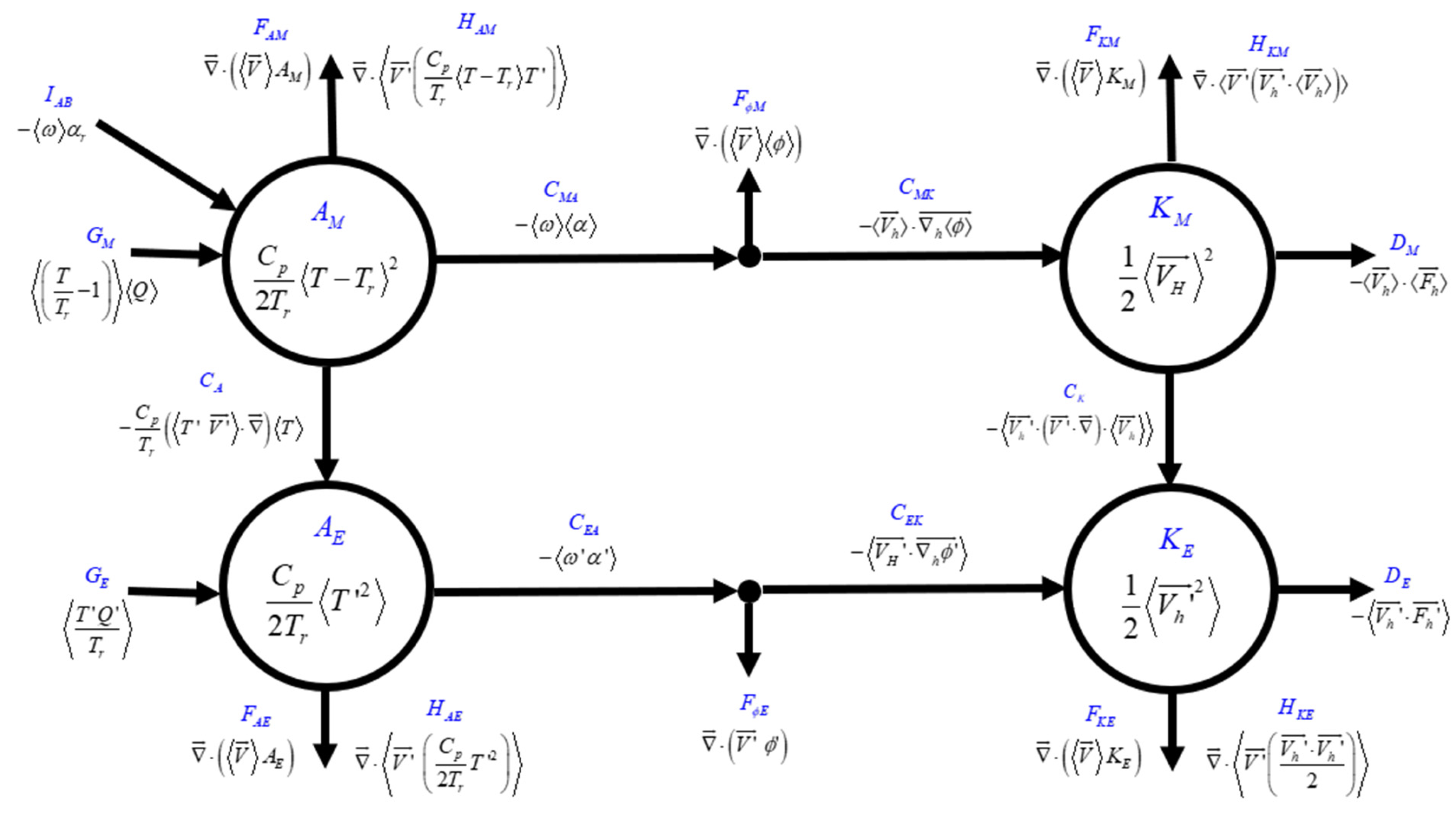
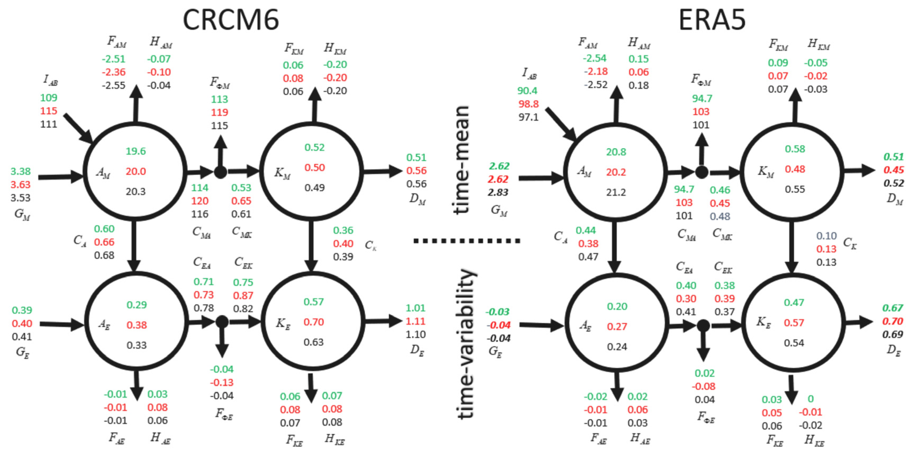
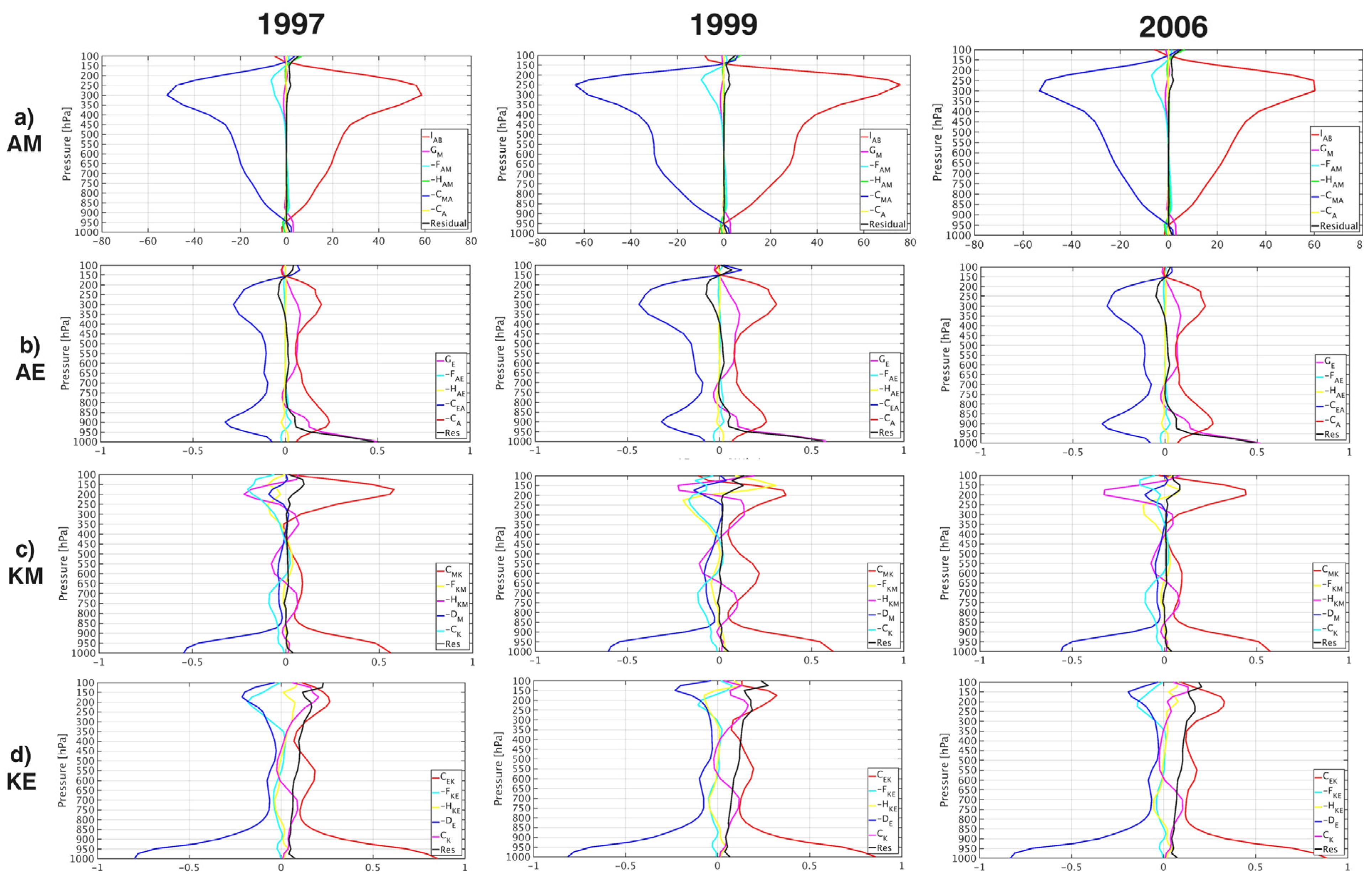
• Boundary flux terms starting with capital letters F or H represent the transport of the energy reservoirs by the time-mean and the time-variability wind (F_AM, H_AM, F_KM, H_KM, F_AE, H_AE, F_KE, H_KE).
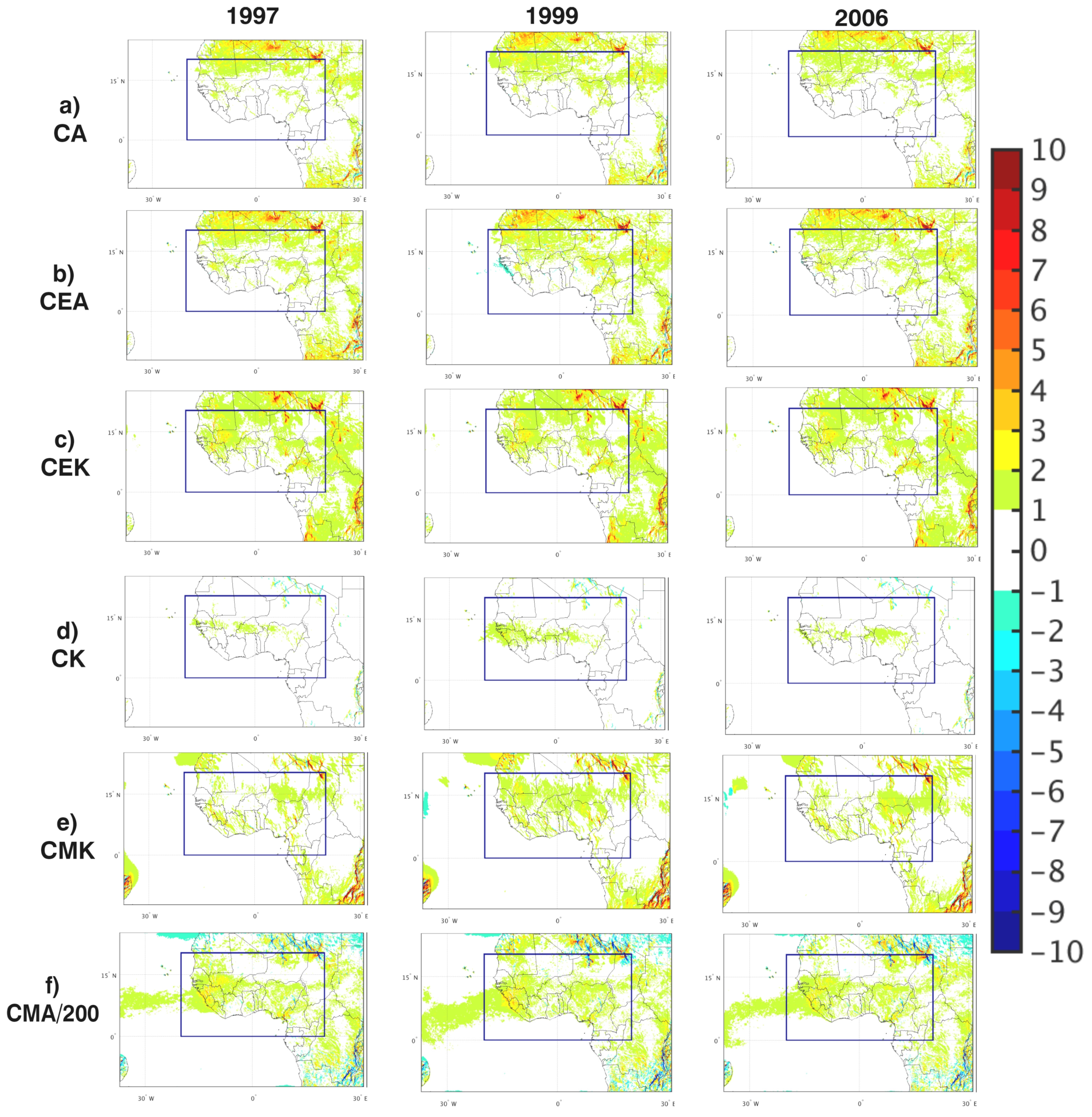
• Conversion terms starting with the capital letter C (C_A, C_K, C_MA, C_MK, C_EA, and C_EK) represent the conversion of energy from one reservoir to another. In regional energy budgets, the presence of lateral boundaries affects the direct conversion from one reservoir to another. As discussed in NLN24, the presence of zero-sum nodes between the available energy and kinetic energy reservoirs implies that the fluxes into kinetic energy C_MK and C_EK differ from the fluxes from available enthalpy C_MA and C_EA. I_AB is also a conversion term resulting from the splitting of the available enthalpy into temperature- and pressure-dependent components.
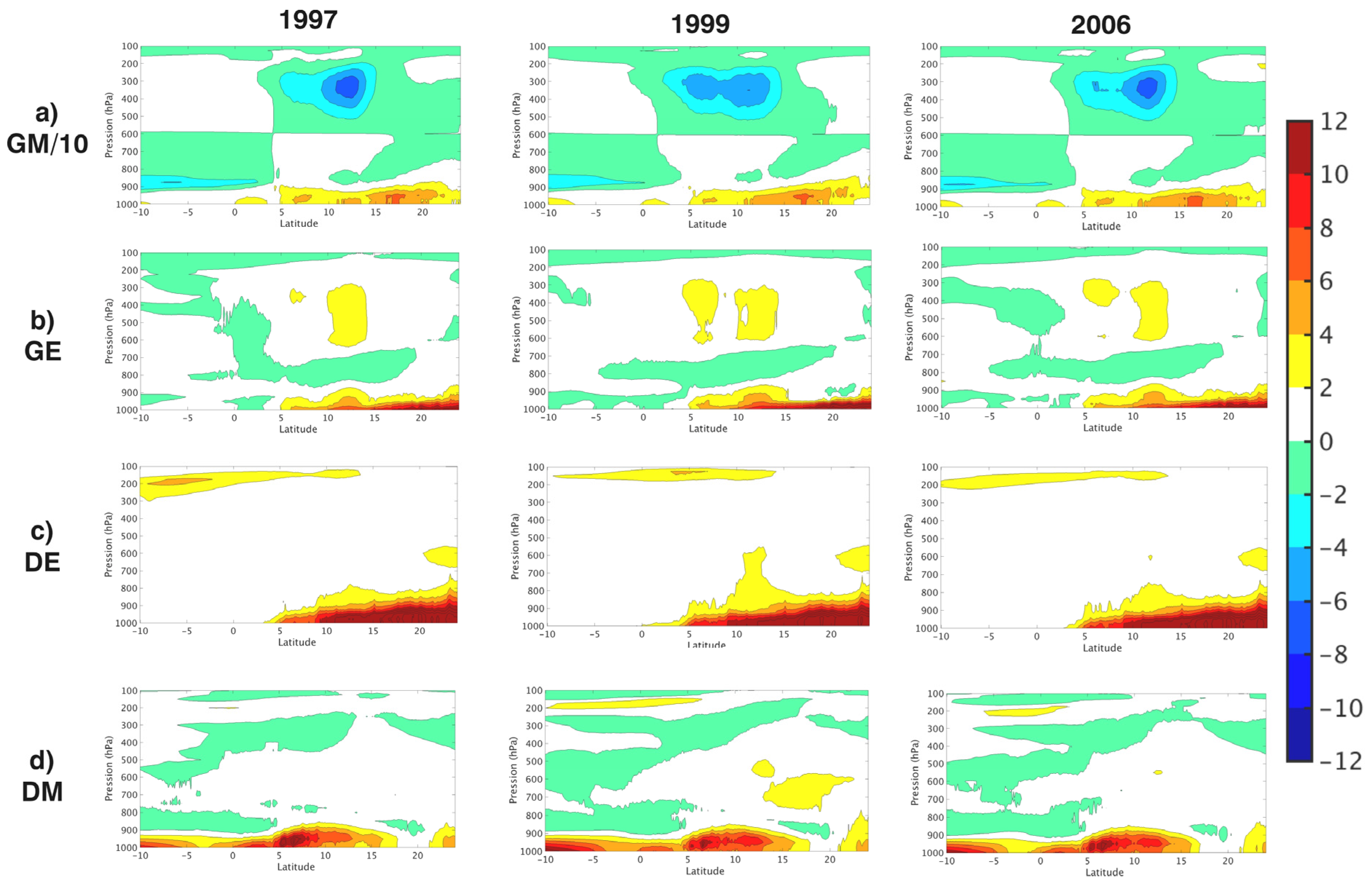
• Generation and dissipation terms start with capital letters G and D (G_M, G_E, D_M, and D_E), respectively. Generation terms are, in general, the main sources of the generation of available enthalpy, while dissipative terms are the main sinks of kinetic energy in the atmosphere.

3. Simulation Configuration and Climate Overview

3.1. Simulation Configuration

The study examines three years that exhibited substantial differences in rainfall amounts during the WAM: 1997 (dry), 1999 (rainy), and 2006 (near normal). A regional climate model (RCM) simulation driven by reanalysis provides high-resolution self-coherent fields required for detailed energetic calculations.

The employed RCM is the sixth-generation Canadian Regional Climate Model (CRCM6/GEM5, [15]) developed at Centre pour l’étude et la simulation du climat à l’échelle régionale of l’Université du Québec à Montréal (ESCER Centre, UQAM). CRCM6/GEM5 is an adapted version of the Global Environmental Multiscale model version 5 (GEM5) from the Meteorological Service of Canada (MSC-ECCC). GEM5 benefits from a major update to the package of physical parameterizations used in Canadian operational Numerical Weather Prediction (NWP), resulting in an improvement of the global energy budget and a reduced sensitivity to the vertical resolution [16]. Of the several horizontal grid options available in GEM5, CRCM6/GEM5 uses the limited-area grid with a rotated latitude–longitude projection. In the vertical, a hybrid hydrostatic pressure coordinate is used [17] with a staggered Charney–Phillips grid.

The subgrid-scale physical parameterization is identical to that used in the operational Canadian NWP Regional Dynamical Prediction System (RDPS, [18]), including the P3 microphysical scheme. The following additional changes were made in CRCM6/GEM5 for our African monsoon simulations. The CLASS land–surface scheme is used, and the thermodynamical column Flake module was used to account for lakes. The grid mesh was coarsened from 0.09° to 0.11° and the uppermost computational level was lowered from 0.1 hPa to 10 hPa. In order to reduce what was perceived as excessive dissipation, the off-centering coefficient of the semi-implicit scheme was reduced from 0.6 to 0.55, and the horizontal diffusion in ${\nabla }^4$ was changed to a ${\nabla }^6$ with a damping coefficient reduced from 0.1 to 0.04.

CRCM6/GEM5 was integrated over a domain comprising the whole West Africa, with a southwest extension to capture Bermuda-Azores anticyclone effect. The domain goes from 37° W to 31° E in longitude and from 12° S to 25° N in latitude (Figure 2). The entire computational domain comprised 660 × 380 points, including a 10-grid-point wide semi-Lagrangian halo and a 10-grid-point wide sponge zone around the 620 × 340 points free domain. In the vertical, 71 terrain-following levels were used, with a top level at 10 hPa. The timestep is 10 min. CRCM6/GEM5 atmospheric lateral boundaries conditions and sea surface temperatures came from the European Centre for Medium-Range Weather Forecasts (ECMWF) ERA5 reanalysis [19], which is based on the Integrated Forecasting System (IFS). ERA5 data are available on an hourly basis on a horizontal grid of 0.25°. In the vertical, there are 27 pressure levels with a finer resolution near the surface. To facilitate the simulation’s evaluation, the CRCM6/GEM5 outputs have been interpolated on the same pressure levels as ERA5. CRCM6/GEM5 simulations covered three sets of seven consecutive months (April to October) for 1997, 1999, and 2006.

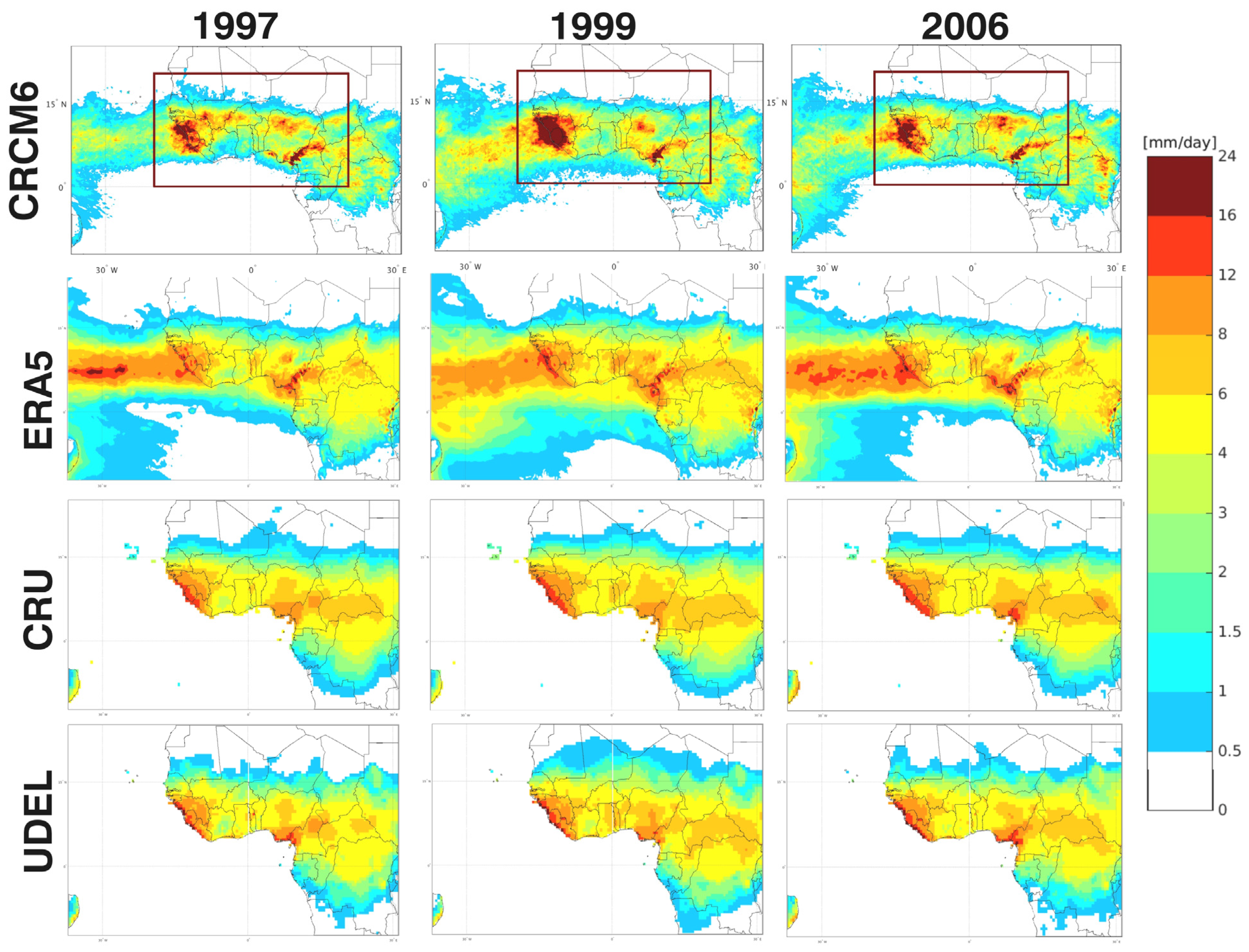
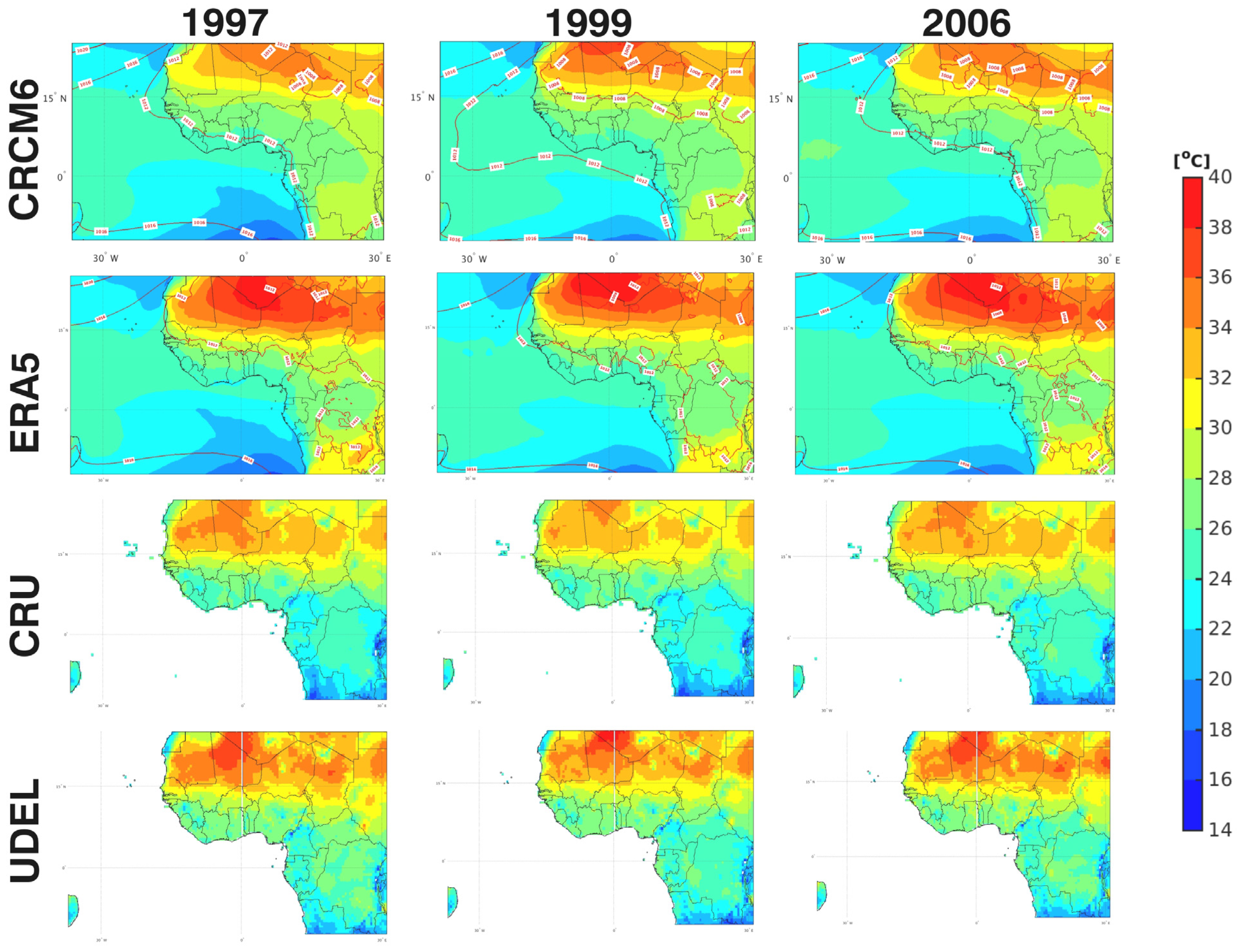
3.2. West African Climate Overview

Previous work performed for the current climate following the CORDEX experimental protocol [7] and for future projections using boundary conditions from a Coupled Global Climate Model (CGCM) [20] provided information on the ability of the model to reproduce the main features of the geographical distribution and seasonal cycle of temperature and precipitation, the diurnal cycle of precipitation, and the WAM. These CGCM-driven regional simulations showed that the model failed to represent properly the cold tongue and brought the WAM rainfall too late over the Sahel region.

In the following, we present an overview of the climate regime over West Africa during three contrasting years (1997/dry, 1999/rainy, and 2006/near normal) from May to September. This description is fundamental to provide a background to the following energetics study. The model simulated results, with a resolution of 0.11°, are compared to ERA5 reanalyzes and gridded analyses of observations such as Climatic Research Unit (CRU, [21]) and University of Delaware Terrestrial Precipitation (UDEL, [22]). May and June have been added to the classical July to September (JAS) monsoon season to capture the pre-onset of the summer monsoon [23].

Figure 3 shows seasonal-mean precipitation fields for each of the three years. Precipitation is an important surface variable in West Africa because of its impact on water resources and food production. In West Africa, precipitation above 4 mm/day is confined between the equator and 15° N. The model simulation overestimates the intensity of precipitation locally, but the overall geographical representation is quite similar to ERA5. There are three main precipitation maxima (above 16 mm/day) in ERA5 and CRCM6 occurring in the Cameroon and Nigeria highlands, the West African coast, and Cape Verde islands. In 1997 (dry), the rainbelt was narrower than in other years, even if precipitation between the equator and 15° N remains high; this confirms that the width of the rainbelt is a better indicator of the monsoon intensity than the annual mean precipitation in the rainbelt.

Figure 4 shows seasonal-mean 2 m surface temperature and mean sea level pressure fields (for ERA5 and the model only). The presence of the hot Sahara in the north of the domain reverses the meridional temperature gradient over West Africa, with lower temperatures located near the Gulf of Guinea and higher temperatures in the Western Sahara (close to the Saharan heat low). In the Gulf of Guinea, the temperature is the highest north of the equator (because of the summer solstice season) and decreases southward. The model simulation is cooler than ERA5 over the continent but is closer to gridded analyses of observations from CRU and UDEL databases over Western Africa. The overall geographical representation is quite similar in observations and simulations. The mean sea level pressure contours in ERA5 and CRCM6/GEM5 show that lower pressures (below 1012 hPa) are located over the continent, especially in the western Sahara. This West African heat low (WAHL) is a key element of the WAM system [24]. In the lower troposphere, the cyclonic circulation associated with the WAHL tends to increase both the southwesterly monsoon flow along its eastern flank and the north-easterly Harmattan flow along its western flank [25]. Over the ocean, Bermuda-Azores and South Atlantic anticyclones dominate, respectively, on the northern and southern sides of the equator.

Figure 5 shows the seasonal-mean vertical cross section of relative humidity and vertical velocity fields. Both ERA5 reanalysis and model simulation show more than 90% relative humidity at the surface from the Gulf of Guinea to 13° N, which coincides with the rainbelt presented in Figure 3. The 90% isohume (line of constant relative humidity) extends further south in 1999 (wet year) than in 1997 (dry year), especially in ERA5, which is in accord with precipitation above 4 mm/day (yellow color) in Figure 3 south of the coast in the Gulf of Guinea. The model simulation succeeds rather well in reproducing the vertical distribution of relative humidity in West Africa. The upper tropospheric maximum vertical velocity near 10° N corresponds to the upward branch of the Hadley cell that transports humidity in the high troposphere. The 1999 (moist year) vertical velocity is stronger than for the other two years. The Hadley cell is distinct from the lower tropospheric vertical velocity cell over the WAHL by its vertical extension. Compared to ERA5, the model simulation appears to overestimate the vertical velocity in both the Hadley cell and the WAHL. The model also underestimates the lower tropospheric rising motion between 15° N and 20° N, but it succeeds in distinguishing its latitudinal limits and vertical extension.

Figure 6 shows the seasonal-mean vertical cross-section of zonal winds. The African Easterly Jet (AEJ) is an important feature of the West African climate. According to the thermal wind relationship, the AEJ is a response to the low-level meridional temperature gradient that forms over West Africa in summer as a result of strong meridional soil moisture gradients [26]. Therefore, the AEJ axis is an indicator of the strong baroclinic zone separating moist and relatively colder Gulf of Guinea regions from dry and hot Saharan regions. Figure 6 shows that mid-tropospheric AEJ position and intensity are well reproduced in the model simulation. AEJ is overall less intense and located further south in 1997 (dry year) compared to 1999 and 2006. The model simulation overestimates the upper-level Tropical Easterly Jet (TEJ) intensity. While the TEJ is significantly correlated with summer Sahel rainfall, its relationship on synoptic to intraseasonal time scales is unclear [27]; hence despite the obvious connection between AEJ and TEJ, this study will focus on the AEJ level.

Figure 7 shows the seasonal-mean vertical cross-section of meridional winds in 1997, 1999, and 2006. Southerly monsoon flow and northerly Harmattan flow converge in the intertropical front (ITF). ITF seasonal-mean position indicates the penetration of the moist monsoonal southwesterlies onto the continent. The model simulation reproduces quite well ITF and the penetration of the monsoon flow in the continent. In the stratosphere, the model overestimates the meridional wind south of 15° N. During the dry year (1997), the monsoonal depth appears thinner and therefore, there is less precipitable water available in the Sahel.

These results show that the CRCM6/GEM5 simulation succeeds in reproducing the overall features of the West African climate. This lends confidence in the energetics calculations performed on the model-simulated fields in the following section.

4. West Africa Energy Budget

Next, we studied the energy cycle climatology of the WAM to unravel the dynamical and physical processes that sustain the summer West African climate. Figure 8 shows time- and domain-averaged values of terms of the energy budget for each of the contrasting years using the CRCM6/GEM5 and the reanalysis. Green, red, and black colors are assigned to the dry (1997), wet (1999) and normal (2006) years, respectively. To focus our analysis on the West Africa domain, terms are horizontally averaged over the sub-domain drawn in Figure 2, vertically integrated from the surface to 600 hPa (which is the mean reference level, where $T\approx T_r=$ 275 K, and time averaged over the period from May to September. With this choice of the vertical eNLxtent and reference temperature, generation term $G_M=〈\left({\displaystyle \frac{T}{T_r}}-1\right)〉 〈Q〉$ has the same sign as diabatic heating, which facilitates the physical interpretation of the energy budget.

An examination of Figure 8 indicates that the energy reservoir A_M is significantly larger than the other reservoirs, by two orders of magnitude. This is due to the effect of the mean stratification of the atmosphere contained in A_M (see [11] Section 6 for details). For this reason, various scales will be employed in the figures presented below to align the terms acting on A_M with those acting on other reservoirs. Both kinetic energy reservoirs K_E and K_M have the same magnitude, suggesting that transient eddy activity is as important as the time-mean for this region of the globe, unlike the case in mid-latitudes where K_M dominates due to the time-mean jet stream. Finally, A_E is the smallest energy reservoir, confirming smaller temperature variations observed in the tropics compared to higher latitudes (~3 × 10⁵ J/s, [28]).

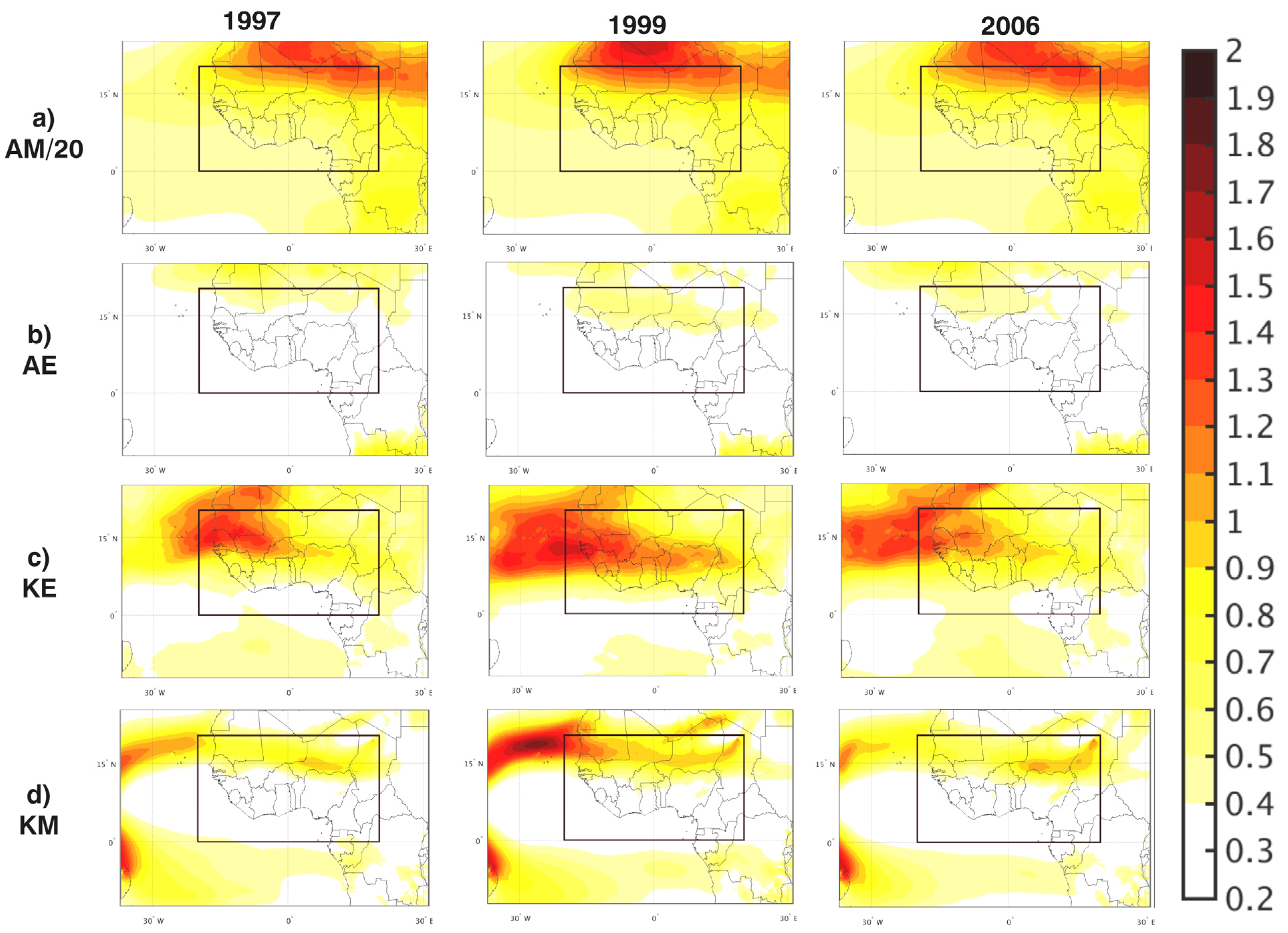
4.1. Analysis of Energy Reservoirs A_M, A_E, K_M, and K_E

Energy reservoirs, depicted by boxes, indicate the average quantity of energy stored within the diagnostic domain. The highest and lowest absolute values reflect more intense and less intense processes, respectively.

4.1.1. A_M

The time-mean available potential energy (A_M) is proportional to the temperature deviation from the reference temperature in the diagnostic domain. Consequently, since the highest values will be located where there is maximum temperature, it is essential to first examine the temperature distribution. Figure 4 shows the seasonal mean 2 m surface temperature. The presence of the hot Sahara in the north of the domain reverses the meridional temperature gradient over West Africa, with lower temperatures located near the Gulf of Guinea and higher temperatures in the Western Sahara (close to the Saharan heat low). In the Gulf of Guinea, the temperature is the highest north of the equator (because of the summer solstice season) and decreases southward. Figure 9a shows seasonal- and longitudinal-mean vertical-latitudinal cross-section of A_M. Values are influenced by the choice of the reference level temperature. In this paper, the reference level has been chosen at 600 hPa to focus on the lower troposphere. Then, there is a gradual increase of A_M away from the reference level. In low levels, there is a maximum of A_M located north of 15° N as a result of high surface temperatures over the Sahara. Note that although the vertical cross-section figures extend up to the 100 hPa level, only values below 600 hPa were taken into account in the energy budget shown Figure 8.

Figure 10a shows a horizontal map of a vertically integrated (from the surface to 600 hPa) A_M field (note the different scale with the other reservoirs). This map is coherent with Figure 9a. In the Sahara region, where the thermal depression is located, significant A_M values are observed, reflecting the high surface temperatures and large lapse rate characteristic of a dry atmosphere. The largest values of A_M over the Sahara were recorded during the wet year of 1999, thereby reinforcing the correlation between the high temperatures in the Saharan boundary layer and the overall WAM system [29]. In contrast, south of 10° N, A_M values are considerably lower, reflecting the smaller lapse rate characteristic of a moist atmosphere. To sum up, the Sahara Desert serves as the primary available enthalpy energy reservoir in West Africa.

4.1.2. A_E

The time-variability available potential energy A_E is proportional to the temperature departure from the time-mean. The seasonal- and longitudinal-mean vertical-latitudinal cross-section of A_E is shown in Figure 9b. The maximum A_E is observed near the surface in northern latitudes and negligible in upper levels. It represents the atmospheric layer where temperature variations are maximum within the season. During the dry year (1997), the maximum of A_E is located north of 20° N and A_E’s vertical penetration is weaker in the Sahel. This is confirmed by the energy budget (Figure 8), where A_E’s lowest values appear during the dry year 1997 and the largest values during the wet year 1999. Generally, during wetter years, the transient-eddy available enthalpy extends further south. Figure 10b shows the vertically integrated A_E map. There is a noteworthy land–sea contrast in the magnitude of A_E, with, in general, lower values over the ocean and larger values over the continent. A_E reflects temperature fluctuations caused by low-level monsoonal winds transporting cool air northward from the Gulf of Guinea and Harmattan winds transporting hot air southward from the Sahara. Over the continent, there is a northward shift of A_E in drier years. In the year characterized by higher precipitation (1999), a latitudinal band near 15° N displays peak values, stretching from Sudan, where AEW’s often originate [30], to the western coast of Africa. It is interesting to note in Figure 8 that contrary to A_M, A_E is higher (lower) in wetter (drier) years, as well in reanalysis as in the model. This clearly suggests that physical mechanisms responsible for the production of A_E are stronger in wetter years. These mechanisms are among the main terms acting on the reservoir A_E (C_A, G_E or C_EA) and will be analyzed in coming sections.

4.1.3. K_E

The time-variability kinetic energy is proportional to the horizontal wind departure from the mean. This term reflects regions where storms are more frequent and is the most interesting energy reservoir for storm studies. Figure 9c shows seasonal- and longitudinal-mean vertical-latitudinal cross-section of K_E. Two maxima are located around the tropopause, corresponding to the equatorial edge of subtropical jets, and another maximum around 650 hPa and 10° N corresponding to the AEJ. In the year characterized by higher precipitation (1999), subtropical wind variance maxima are closed, compared to other years. Figure 10c shows the vertically integrated (from the surface to 600 hPa) K_E field. Over the continent, maximum values near 10° N correspond to the AEJ, which is a response to the strong meridional temperature gradient at the surface. This maximum originates to South Sudan and intensifies westward off the west coast, especially during wetter years. It is interesting to note, as was the case with A_E, that maximum values over the continent start from Sudan, where AEWs often originate [30]. On the West coast, there is a mix between those values and systems coming from mid-latitudes. This supply of energy is important for the development of systems in tropical cyclones in the Atlantic.

Close to the equator, low values characteristics of doldrums are observed. In 1999, K_E maximum west of Cape Verde Islands confirms the intense Atlantic hurricane season reported in the literature, with five Category 4 hurricanes—the third largest number recorded in a single season in the Atlantic basin between 2005 and 2020. It is interesting to see how K_E values in the model and the reanalysis (Figure 8) are proportional to the precipitation activity despite the fact that K_M values are not. This once again suggests that the main physical processes acting on the generation of time-variability kinetic energy K_E (C_K, C_EK or D_E) are linked with the precipitation activity during the African monsoon. These terms will be investigated in the coming sections.

4.1.4. K_M

The time-mean kinetic energy is proportional to the mean horizontal wind. Figure 6 and Figure 7 illustrate, respectively, the seasonal-mean vertical cross-section of zonal and meridional winds. The African Easterly Jet (AEJ) is an important feature of the West African climate. According to the thermal wind relationship, the AEJ is a response to the low-level meridional temperature gradient that forms over West Africa in summer as a result of strong meridional soil moisture gradients [28]. Therefore, the AEJ axis is an indicator of the strong baroclinic zone separating moist and relatively colder Gulf of Guinea regions from dry and hot Saharan regions. Figure 6 illustrates that mid-tropospheric AEJ position and intensity are well reproduced in the model simulation. AEJ is overall less intense and located further south in 1997 (dry year) compared to 1999 and 2006. The simulation overestimates the upper-level Tropical Easterly Jet (TEJ) intensity. While the TEJ is significantly correlated with the summer Sahel rainfall, its relationship on synoptic to intraseasonal time scales is unclear [27]; hence despite the obvious connection between AEJ and TEJ, this study will focus on the AEJ level. That is why the vertical mean in the computation of terms in Figure 8 is from the surface to 600 hPa. Figure 9d shows seasonal- and longitudinal-mean vertical-latitudinal cross-section of K_M. Maximum time-mean energy is associated with the upper levels of jet streams. At 600 hPa, there is the AEJ, which is more intense and with a larger latitudinal extend during wetter years (1999 and 2006). At 200 hPa, near the tropopause, there is the TEJ in the center of the domain, which is clearly connected with the AEJ. It is particularly intense during the wetter year (1999) and would have obviously played a strong role in the development of the AEJ and precipitations. The zonal wind component dominates K_M energy reservoir, so that the distribution of K_M is not visibly affected by the maximum of the meridional wind near the surface and its minimum close to the tropopause. Figure 10d shows maps of vertically integrated (from the surface to 600 hPa) K_M field. Maximum values on the continent are located around 15° N, in the trajectory of the AEJ and are somewhat larger during the wet year of 1999. K_M magnitude increases westward from the coast to reach a maximum over the Atlantic. It is interesting to note that the time-mean kinetic energy is higher in both ERA5 and the model during the dryer year.

4.2. Conversion Terms

In this section, we analyze terms responsible for conversion between energy reservoirs. C_A converts available enthalpy energy from time-mean A_M to time-variability A_E. Figure 11a shows the seasonal- and longitudinal-mean vertical-latitudinal cross-section of C_A, where two distinct maxima are noticeable. One maximum is located near 12° N and extends up to the tropopause; it reflects the upward branch of the Hadley cell with deep moist convection. The other maximum extends from the surface up to 600 hPa north of the Sahel; it reflects the shallow dry convection that develops in the Sahara due to high insolation.

As to be expected, the latitudinal extent and intensity of the deep convection are larger during the wetter year (1999) than in other years, confirming that in the wet years, the rainbelt is markedly more intense and its core covers a wider latitudinal band [31]. The dry convection shows low interannual variability. The results confirm that, on a long-time scale, the time-mean feeds the eddies, the positive values of C_A indicate that the conversion goes from A_M to A_E. C_A is dominated by its vertical component due to the strong vertical temperature variations compared to horizontal temperature gradients in the tropical atmosphere.

Figure 12a shows a map of the vertically integrated (from the surface to 600 hPa) C_A field. Positive values occur over most of the domain, confirming that A_M is converted to A_E, with maximum conversion occurring over the Sahara. Note that the presence of stationary local hotspots for all three years suggests a numerical artifact due to the computation of the vertical motion near the surface. Figure 11a shows the seasonal- and longitudinal-mean vertical-latitudinal cross-section of C_A. The conversion within the Saharan boundary layer appears to be more pronounced during wetter years, explaining C_A’s values observed in Figure 8. C_A is also more intense in upper levels in the Hadley cell during wetter years, but it does not influence our results, due to our vertical integration limit set at 600 hPa.

C_EA is the flux of A_E that is offered for conversion into K_E, through rising (sinking) of warm (cold) anomalies in the atmosphere. It indicates the covariance of the temperature and the vertical motion. Figure 11b shows the seasonal- and longitudinal-mean vertical-latitudinal cross-section of C_EA. This field is quite similar to C_A, which should not be surprising given that it is proportional to C_A’s vertical component (see “Appendix A” for details). Figure 5 shows the seasonal-mean vertical cross-section of relative humidity and vertical velocity fields. We see an important upward vertical activity in the Hadley cell and subsidence elsewhere. We also confirm that the secondary maximum in the Sahara lower troposphere is the shallow dry convection that develops in the Sahara due to high insolation. Finally, it is interesting to note that in every year the model simulation overestimated the vertical motion compared to ERA5. This explains why in Figure 8, C_EA is systematically greater than C_A in the model and the reverse in reanalysis.

C_EK represents physically the horizontal ageostrophic term expressing local imbalances between time-variability pressure gradient and time-variability Coriolis force. In Figure 8, we see that the zero-sum node between C_EA and C_EK exhibits a very small contribution from boundary flux F_ϕE, which means that there is little overall pressure work acting at the lateral boundaries for transient eddies, and hence C_EA is nearly equal to C_EK. This implies that the loss of A_E contributes almost entirely to the gain in K_E, when integrated over the limited-area diagnostic domain. Figure 11c shows the seasonal- and longitudinal-mean vertical-latitudinal cross-section of C_EK. Despite the fact that C_EA is nearly equal to C_EK when integrated over the limited-area domain, their vertical-latitudinal cross-sections exhibit notable differences (Figure 11b,c). The large maximum C_EK located in the low levels north of 5° N reflects the fluctuations of the mass convergence toward the fluctuating SHL. Two secondary maxima are located on both sides of the Saharan desert, at around 600 hPa. This reflects the well-known structure of the Saharan circulation [32], where mass converges into the near-surface low, ascends, and diverges out of the lower mid-tropospheric high in an ageostrophic overturning circulation; this shallow overturning extends across the entire Sahara desert [33]. Figure 12c shows a map of the vertically integrated (from the surface to 600 hPa) C_EK field; we can see that C_EK is nearly equal to C_EA. It is interesting to see in Figure 8, both in the model simulation and reanalyzes, how boundary fluxes contribute to C_EK during wet years. This indicates that the ageostrophic term is linked to the mean precipitation.

C_K is the conversion flux between K_M and K_E. A positive value of C_K implies a barotropic conversion from the time-mean state to transient eddies. Figure 11d shows seasonal- and longitudinal-mean vertical-latitudinal cross-section of C_K. In the lower part of the troposphere, C_K is mostly positive, with two distinct maxima. The strongest one is located near 800 hPa and 12° N, below the AEJ level; it therefore indicates that the AEJ plays a key role in the development and maintenance of AEWs. The second weaker maximum is just above the Sahara’s surface, north of 15° N, related to the heat low during the summer season [34]. Other maxima occurring near the tropopause are related to transient eddies around subtropical jets in the southern and northern hemispheres; being above 600 hPa, these will not be considered in the computation of the energy budget. Figure 12d shows the vertically integrated (from the surface to 600 hPa) C_K map. Values are positive in almost all the domains, with maximum values on the West African coast in the trajectory of AEWs and in the Sahara, as illustrated in vertical cross-section maps. Despite the fact that time-mean kinetic energy is higher in reanalysis, conversion from K_M to K_E is higher in the model simulation, with maximum (minimum) values in wetter (dryer) years.

C_MK is the energy flux affecting the time-mean kinetic energy K_M from available enthalpy A_M. Physically, C_MK represents the horizontal ageostrophic term expressing any local imbalances between the time-mean pressure gradient and Coriolis force. Figure 11e shows seasonal- and longitudinal-mean vertical-latitudinal cross-section of C_MK. Positive conversions (meaning contribution to increase K_M) occur near the surface, in mid- and upper levels. Surface maxima are related to the monsoonal flow activity, with southerlies bringing humidity in the Sahel. Mid-level and upper maxima are associated with the ageostrophic circulations around, respectively, the AEJ, the TEJ and mid-latitudes jets. It is interesting to see the similarity between the time-mean and the time-variability production of kinetic through C_MK and C_EK, respectively (Figure 8); this confirms the relevance of the time-mean ageostrophic circulation to understand the variability of the jet and how it is maintained [26]. Figure 12e shows the vertically integrated C_MK map; due to the vertical integration limits from the surface to 600 hPa, only the AEJ ageostrophic circulation appears. There is a maximum conversion during the wetter years, with a larger latitudinal extent around the AEJ mean position at 15° N.

We note in Figure 8 that in the zero-sum node between C_MA and C_MK, the boundary flux F_ϕM is very large, probably due to the increase in the geopotential with height as a consequence of the stratification of the atmosphere; this means that only a very small fraction of the conversion C_MA from time-mean available enthalpy A_M contributes to increasing the time-mean kinetic energy K_M through C_MK. C_MA converts A_M into K_M by upward transport of warm and humid air from the surface to the top of the troposphere. As shown in Figure 11f (note the different scale of this panel), this phenomenon is particularly strong in the ITCZ. Positive values from 3° N to 17° N delimitate the ascending branch of the Hadley cell, while negative values indicate the subsiding branch in southern and northern boundaries of the domain. North of 17° N there is a shallow meridional overturning cell—as described in [35]—with positive C_MA values due to the upward motion of warm and dry air in the thermal depression, and negative C_MA values due to the descending branch of the Hadley cell. Figure 12f shows the vertically integrated (from the surface to 600 hPa) C_MA map (note again the different scale of this panel). Over the continent, the calculation of C_MA is challenging, due to the presence of topography, which results in excessively large (unrealistic) fluctuations of alternating sign. Over the ocean, the Hadley cell contributes to positive values; it was narrower in 1997 compared to wetter years. However, it should be noted that because the boundary flux F_ϕM is very large at the zero-sum node (Figure 8), only a very small fraction of the conversion C_MA contributes to C_MK increasing K_M.

4.3. Energy Generation and Dissipation Terms

We now present the details of the physical terms contributing to the generation or dissipation of energy reservoirs. These terms are only available in the model simulation. A correct physical interpretation of generation terms depends on the knowledge of terms contributing to Q. Figure 13 and Figure 14 show, respectively, the vertical cross-section and vertically integrated maps of processes contributing to Q.

Figure 14 shows that convection is intense in the Hadley cell, especially in the oceanic boundary layer. Figure 13 shows that the condensation is intense and confined in the Sahel (between 5 and 15° N) in the upper levels, but this dominance is not visible on maps (Figure 14b) due to the upper limit fixed at 600 hPa. Radiation is dominant over the ocean and vertical diffusion is dominant on the continental surface, especially in the Sahara.

With this overview of contributing terms, we can now analyze generative and dissipative terms.

Because of the definition of $G_M=〈\left({\displaystyle \frac{T}{T_r}}-1\right)〉 〈Q〉$, the diabatic generation of A_M will be of the same sign as the diabatic heating rate Q below the reference level, and of different sign above the reference level. Figure 15a shows seasonal- and longitudinal-mean vertical-latitudinal cross-section of G_M. There is generation of A_M below 800 hPa in the boundary layer north of the equator. There is a maximum over the Sahara Desert, mainly due to sensible surface heat flux and vertical diffusion (Figure 13d). South of the equator and around 900 hPa, there is a dissipation of A_M as a consequence of the radiative cooling (Figure 13c). The dissipation of A_M at the tropopause near 10° N is a consequence of warming by condensation and convection (Figure 13a,b and Figure 14a,b).

Figure 16a shows the vertically integrated (below 600 hPa) G_M map. Over the continent, positives values over the Sahara (and to a lesser extent in the southern hemisphere) are due to sensible surface heat flux and vertical diffusion (Figure 13d). The maximum generation of A_M over the ocean off the West African coast is mostly the consequence of latent heat release (Figure 13b) associated with precipitation.

Figure 15b shows the seasonal- and longitudinal-mean vertical-latitudinal cross-section of G_E, the generation of A_E, which reflects the covariance of diabatic heating and temperature fluctuations. This component reflects regions where temperature variations are correlated with variations in diabatic heating rate. The low-level maximum G_E, north of 5° N, results from the positive covariance of perturbations of temperature and diabatic heating by radiation (Figure 13c) and vertical diffusion of heat (Figure 13d). Figure 16b shows the vertically integrated (below 600 hPa) G_E map; maximum values are noted in the continent where there is topography. This suggests an important role of the surface sensible heat flux and vertical diffusion of heat (Figure 13d). Due to the integration upper limit, the deep convection occurring above 600 hPa in (Figure 14b) does not contribute.

Figure 15c shows the seasonal- and longitudinal-mean vertical-latitudinal cross-section of D_E, the dissipation of K_E through friction stress at the surface, and turbulent diffusion above. The largest energy dissipation occurs near the surface north 8° N as the result of the covariance of perturbations of horizontal winds and surface stress. Figure 15c shows the vertically integrated D_E map. The values are particularly large north of 13° N, in the Sahara, where time fluctuations of surface stress and low-level winds associated with the heat low are maximum. South of 15° N, there is another maximum of D_E in the Cameroonian and Nigerian highlands.

Figure 15d shows the seasonal- and longitudinal-mean vertical-latitudinal cross-section of D_M, the dissipation of K_M through stress at the surface. The maximum D_M values are found in the low levels and their position coincides with low-level monsoon winds, as shown in Figure 7. This suggests that friction acting upon monsoon winds contributes to the dissipation of K_M. Figure 16d shows the vertically integrated D_M map. No clear maximum is noted, because of the lower magnitude of D_M compared to D_E.

4.4. Boundaries Fluxes Terms

In a regional energy budget, energy fluxes across the diagnostic domain perimeter need to be taken into account. Despite the use of the 600 hPa as the upper diagnostic domain limit, the boundary fluxes are dominated by horizontal transport rather than the vertical one. Figure 8 shows that the largest boundary fluxes are I_AB into A_M and F_ϕM out of the zero-sum node between A_M and K_M. In fact, these very large values are linked with similarly large C_MA conversion flux values. Hence, this part of the energy cycle diagram is of little interest because boundary fluxes largely dominate over processes occurring within the diagnostic domain. Other boundary flux terms are smaller than conversion or generation/dissipation terms, and hence will not be discussed further.

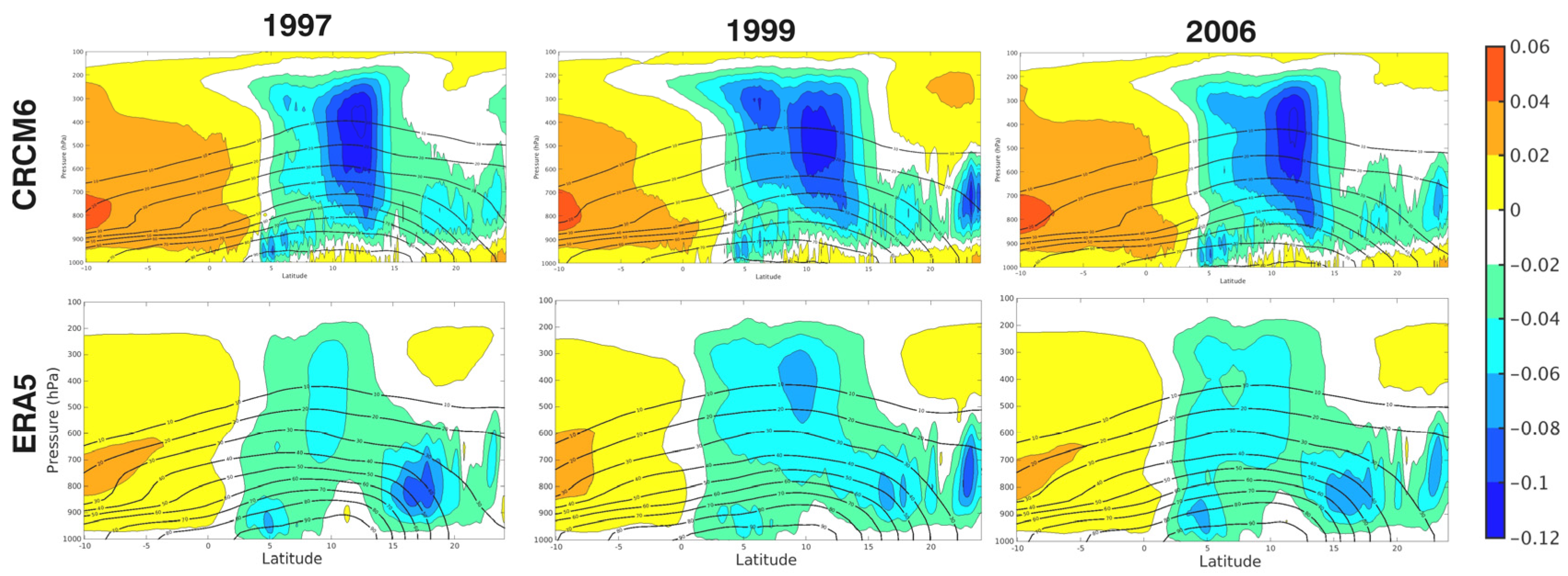
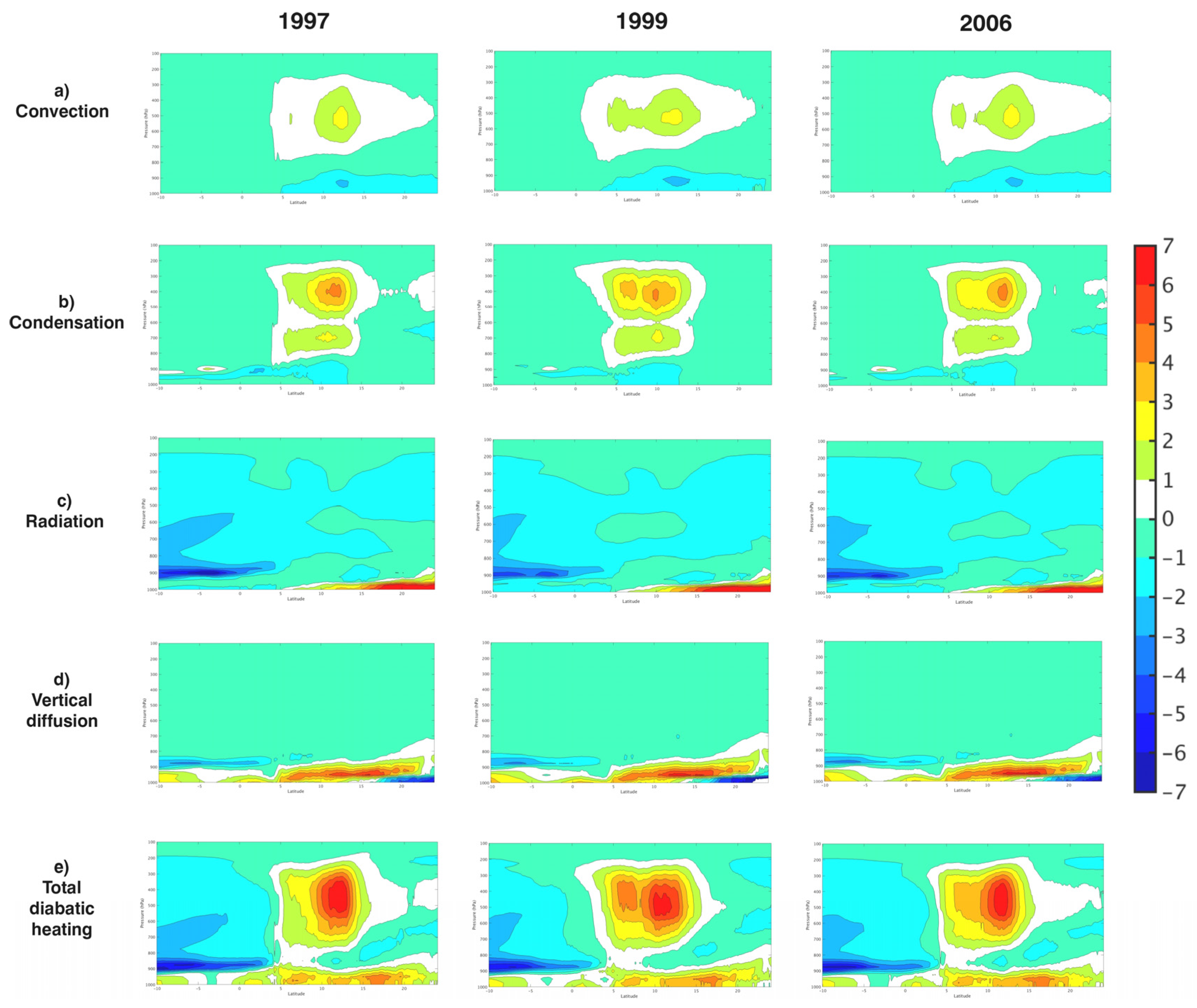
4.5. Vertical Profiles

Figure 17 shows the vertical profiles of time-mean (May–September) and horizontally averaged (20° W–20° E; 0–20° N) values of the four energy reservoirs, A_M, A_E, K_M, and K_E. Colored lines represent individual contributions acting upon each energy reservoir and black lines represent the residual, the sum of the contributions to reservoirs. The residual should, in theory, be nearly equal to zero; this is not the case due to numerical errors.

Figure 17a shows the various contributions to the time tendency of A_M (note the different scales used for A_M). Contributions I_AB and C_MA dominate the energy budget, as mentioned above, confirming the energy equilibrium shown in Figure 3. During wetter years, conversion terms I_AB and C_MA are larger as the consequence of a more intense Hadley cell activity. The generation of diabatic heating G_M is important below 900 hPa, with some noise due to the presence of the topography.

Figure 17b shows the various contributions to the time tendency of A_E. The mean equilibrium for A_E appears to result from compensation, with C_A and G_E adding up to feed C_EA. Conversion terms C_A and C_EA, and the generation term G_E, dominate the A_E budget on average over the domain, as shown in Figure 3, and boundary fluxes terms are negligible. Hence, C_A and G_E add up to feed C_EA. The positive residual in the boundary layer reveals again the numerical computing issue in closing the energy budget. The interannual variability is larger in the upper levels, with conversion contributions being stronger during wet years.

Figure 17c shows the various contributions to the time tendency of K_M. Compensation occurs between the different contributions, depending upon the level. Below 850 hPa, the time-mean ageostrophic circulation source term C_MK counterbalances the frictional term D_M as to be expected in the Ekman layer balance. Between 800 and 400 hPa, the barotropic conversion C_K also contributes to the balance between C_MK and D_M, with some contribution from the boundary term H_KM. During wetter years, various contributions to the local tendency of K_M increase in agreement with the AEJ intensity noted in Figure 9d and Figure 10d.

Figure 17d shows the various contributions to the time tendency of K_E. In the boundary layer, the main balance is between the ageostrophic circulation conversion term C_EK and the frictional sink term D_M, reflecting wind convergence in low pressures. Below the AEJ level, the time-variability ageostrophic conversion term C_EK and the barotropic conversion term C_K are the main source of production of K_E and therefore contribute to the growth and maintenance of the AEWs, whereas the dissipative term D_E acts as the main dissipation of time-variability kinetic energy. There is a low interannual variability between wet and dry years. We note that the time tendency, which should nearly vanish, increases slightly gradually from the ground, as a result of inaccuracies in the calculation of the several contributions that are summed up.

5. Summary and Conclusions

An evaluation of three contrasting West African monsoon seasons was carried out using the sixth generation of the Canadian Regional Climate Model (CRCM6/GEM5), driven by ERA5 reanalyzes from ECMWF. We adapted the formalism developed by NLN24 for regional-scale atmospheric energetics studies. This approach is expected to reveal mechanisms responsible for intraseasonal variability observed during three contrasting years (1997/dry, 1999/wet, and 2006/moderate).

The model simulation was first evaluated against ERA5 reanalyzes, and the results indicate that the model was able to represent the main seasonal features of the West African monsoon. The energy budgets of the simulation and reanalysis also indicate consistency. It is important to note that ERA5 physical terms (diabatic heating rate and friction) were not available to us. We computed them as residuals of thermodynamic and momentum equations; for this reason, the ERA5 energy budget was not analyzed here.

The model simulation energy path shows that A_M dominates other energy reservoirs, its magnitude reflecting the high surface temperatures and lapse rate characteristic of a dry atmosphere. Apart from dominant terms (I_AB, C_MA) acting on A_M and F_ϕM at the zero-sum node, which are not meaningful for the understanding of the energy budget, the generation of diabatic heating by the time-mean G_M is the main source of energy in West Africa. This generation of A_M through diabatic processes is counteract by conversion of A_M into K_M (through C_MK) and A_E (through C_A). Therefore, both A_M into K_M contribute to the generation of eddy kinetic energy through C_K and C_EK, respectively. Finally, the dissipative term D_E is the main terms that counteract the generation of K_E and acts to dampen the creation of AEW’s. From the energetics point of view, the time-mean part the time-mean part of the energy budget (upper part of Figure 9), contrary to the time-variability, does not generally reflect the intraseasonal variability of the West African monsoon. On the other hand, transient-eddy energy reservoirs (A_E and K_E) values are low during dry years, high during wet years, and medium during moderate years. This is also the case of terms responsible for the conversion of energy into eddy kinetic energy K_E (C_K and C_EK), as well as the dissipative term C_K. Physically, the conversions C_MK and C_EK are ageostrophic terms expressing local imbalances between pressure gradient and Coriolis force.

While at the global scale, the conversion from A_M to K_M and A_E to K_E is direct, due to the absence of boundary flux terms at the zero-sum nodes, the regional energy budget formulation proposed by NLN24 has the advantage of showing the fraction of conversion from A_M and K_M responsible, respectively, to the generation of A_E and K_E.

In view of all the foregoing, time-variability energy budget highlights physical processes responsible for the production of AEWs and therefore precipitation activity over West Africa. Monitoring time-variability energy budget in seasonal forecasts could contribute to reducing vulnerability to drought and floods in West Africa, in general, and in the Sahel especially. From a climate-change perspective, the regional atmospheric energy budget could be applied to climate projections to study how the various processes will evolve in a future climate. Atmospheric energetic equations are powerful tools to evaluate a wide spectrum of temporal scales, in particular in regions with a dearth of long-term in situ data, such as West Africa. Our forthcoming work will focus on the study of the life cycle of African Easterly Waves (AEW), aiming to understand mechanisms responsible for the generation, maintenance, and dissipation of an AEW using the high-resolution CRCM6/GEM5 driven by ERA5 and making use of the formalism developed by NLN24 for weather systems.

References

1. Gowing, J.W. Food security for sub-Saharan Africa: Does water scarcity limit the options? Land Use Water Resour. Res. 2003, 3. [Google Scholar] [CrossRef]
2. Redelsperger, J.-L.; Thorncroft, C.D.; Diedhiou, A.; Lebel, T.; Parker, D.J.; Polcher, J. African Monsoon Multidisciplinary Analysis: An international research project and field campaign. Bull. Am. Meteorol. Soc. 2006, 87, 1739–1746. [Google Scholar] [CrossRef]
3. Lebel, T.; Parker, D.J.; Flamant, C.; Bourlès, B.; Marticorena, B.; Mougin, E.; Peugeot, C.; Diedhiou, A.; Haywood, J.; Ngamini, J.-B. The AMMA field campaigns: Multiscale and multidisciplinary observations in the West African region. Q. J. R. Meteorol. Soc. 2010, 136, 8–33. [Google Scholar] [CrossRef]
4. Hourdin, F.; Musat, I.; Guichard, F.s.; Ruti, P.M.; Favot, F.; Filiberti, M.-A.; Pham, M.; Grandpeix, J.-Y.; Polcher, J.; Marquet, P. AMMA-model intercomparison project. Bull. Am. Meteorol. Soc. 2010, 91, 95–104. [Google Scholar] [CrossRef]
5. Boone, A.; De Rosnay, P.; Balsamo, G.; Beljaars, A.; Chopin, F.; Decharme, B.; Delire, C.; Ducharne, A.; Gascoin, S.; Grippa, M. The AMMA land surface model intercomparison project (ALMIP). Bull. Am. Meteorol. Soc. 2009, 90, 1865–1880. [Google Scholar] [CrossRef]
6. Xue, Y.; De Sales, F.; Lau, W.-M.; Boone, A.; Feng, J.; Dirmeyer, P.; Guo, Z.; Kim, K.-M.; Kitoh, A.; Kumar, V. Intercomparison and analyses of the climatology of the West African Monsoon in the West African Monsoon Modeling and Evaluation project (WAMME) first model intercomparison experiment. Clim. Dyn. 2010, 35, 3–27. [Google Scholar] [CrossRef]
7. Hernández-Díaz, L.; Laprise, R.; Sushama, L.; Martynov, A.; Winger, K.; Dugas, B. Climate simulation over CORDEX Africa domain using the fifth-generation Canadian Regional Climate Model (CRCM5). Clim. Dyn. 2013, 40, 1415–1433. [Google Scholar] [CrossRef]
8. Lorenz, E.N. Available potential energy and the maintenance of the general. Tellus 1955, 7, 157–167. [Google Scholar] [CrossRef]
9. Li, L.; Ingersoll, A.P.; Jiang, X.; Feldman, D.; Yung, Y.L. Lorenz energy cycle of the global atmosphere based on reanalysis datasets. Geophys. Res. Lett. 2007, 34. [Google Scholar] [CrossRef]
10. Ngueto, Y.F.; Laprise, R.; Nikiéma, O. A Detailed Limited-Area Atmospheric Energy Cycle for Climate and Weather Studies. Atmosphere 2024, 15, 87. [Google Scholar] [CrossRef]
11. Nikiéma, O.; Laprise, R. An approximate energy cycle for inter-member variability in ensemble simulations of a regional climate model. Clim. Dyn. 2013, 41, 831–852. [Google Scholar]
12. Thorncroft, C.; Hoskins, B. An idealized study of African easterly waves. II: A nonlinear view. Q. J. R. Meteorol. Soc. 1994, 120, 983–1015. [Google Scholar] [CrossRef]
13. Kebe, I.; Diallo, I.; Sylla, M.B.; De Sales, F.; Diedhiou, A. Late 21st century projected changes in the relationship between precipitation, African easterly jet, and African easterly waves. Atmosphere 2020, 11, 353. [Google Scholar] [CrossRef]
14. Lorenz, E.N. Energy and numerical weather prediction. Tellus 1960, 12, 364–373. [Google Scholar]
15. Roberge, F.; Di Luca, A.; Laprise, R.; Lucas-Picher, P.; Thériault, J. Spatial spin-up of precipitation in limited-area convection-permitting simulations over North America using the CRCM6/GEM5. 0 model. Geosci. Model Dev. 2024, 17, 1497–1510. [Google Scholar]
16. McTaggart-Cowan, R.; Vaillancourt, P.; Zadra, A.; Chamberland, S.; Charron, M.; Corvec, S.; Milbrandt, J.; Paquin-Ricard, D.; Patoine, A.; Roch, M. Modernization of atmospheric physics parameterization in Canadian NWP. J. Adv. Model. Earth Syst. 2019, 11, 3593–3635. [Google Scholar]
17. Laprise, R. The Euler equations of motion with hydrostatic pressure as an independent variable. Mon. Weather Rev. 1992, 120, 197–207. [Google Scholar]
18. Milbrandt, J.; Morrison, H. Parameterization of cloud microphysics based on the prediction of bulk ice particle properties. Part III: Introduction of multiple free categories. J. Atmos. Sci. 2016, 73, 975–995. [Google Scholar] [CrossRef]
19. Hersbach, H.; Bell, B.; Berrisford, P.; Hirahara, S.; Horányi, A.; Muñoz-Sabater, J.; Nicolas, J.; Peubey, C.; Radu, R.; Schepers, D. The ERA5 global reanalysis. Q. J. R. Meteorol. Soc. 2020, 146, 1999–2049. [Google Scholar]
20. Hernández-Díaz, L.; Laprise, R.; Nikiéma, O.; Winger, K. 3-Step dynamical downscaling with empirical correction of sea-surface conditions: Application to a CORDEX Africa simulation. Clim. Dyn. 2017, 48, 2215–2233. [Google Scholar] [CrossRef]
21. Harris, I.; Osborn, T.J.; Jones, P.; Lister, D. Version 4 of the CRU TS monthly high-resolution gridded multivariate climate dataset. Sci. Data 2020, 7, 109. [Google Scholar] [PubMed]
22. Matsuura, K.; Willmott, C. University of Delaware Terrestrial Precipitation; NOAA ESRL: Boulder, CO, USA, 2018. [Google Scholar]
23. Sultan, B.; Janicot, S.; Diedhiou, A. The West African monsoon dynamics. Part I: Documentation of intraseasonal variability. J. Clim. 2003, 16, 3389–3406. [Google Scholar]
24. Lavaysse, C.; Flamant, C.; Janicot, S.; Parker, D.J.; Lafore, J.-P.; Sultan, B.; Pelon, J. Seasonal evolution of the West African heat low: A climatological perspective. Clim. Dyn. 2009, 33, 313–330. [Google Scholar]
25. Parker, D.J.; Thorncroft, C.D.; Burton, R.R.; Diongue-Niang, A. Analysis of the African easterly jet, using aircraft observations from the JET2000 experiment. Q. J. R. Meteorol. Soc. A J. Atmos. Sci. Appl. Meteorol. Phys. Oceanogr. 2005, 131, 1461–1482. [Google Scholar]
26. Cook, K.H. Generation of the African easterly jet and its role in determining West African precipitation. J. Clim. 1999, 12, 1165–1184. [Google Scholar] [CrossRef]
27. Lemburg, A.; Bader, J.; Claussen, M. Sahel rainfall–tropical easterly jet relationship on synoptic to intraseasonal time scales. Mon. Weather Rev. 2019, 147, 1733–1752. [Google Scholar]
28. Clément, M.; Nikiéma, O.; Laprise, R. Limited-area atmospheric energetics: Illustration on a simulation of the CRCM5 over eastern North America for December 2004. Clim. Dyn. 2017, 48, 2797–2818. [Google Scholar]
29. Lavaysse, C.; Flamant, C.; Janicot, S.; Knippertz, P. Links between African easterly waves, midlatitude circulation and intraseasonal pulsations of the West African heat low. Q. J. R. Meteorol. Soc. 2010, 136, 141–158. [Google Scholar]
30. Mekonnen, A.; Thorncroft, C.D.; Aiyyer, A.R. Analysis of convection and its association with African easterly waves. J. Clim. 2006, 19, 5405–5421. [Google Scholar]
31. Nicholson, S.E. The intensity, location and structure of the tropical rainbelt over west Africa as factors in interannual variability. Int. J. Climatol. A J. R. Meteorol. Soc. 2008, 28, 1775–1785. [Google Scholar]
32. Thorncroft, C.D.; Nguyen, H.; Zhang, C.; Peyrillé, P. Annual cycle of the West African monsoon: Regional circulations and associated water vapour transport. Q. J. R. Meteorol. Soc. 2011, 137, 129–147. [Google Scholar] [CrossRef]
33. Shekhar, R.; Boos, W.R. Weakening and shifting of the Saharan shallow meridional circulation during wet years of the West African monsoon. J. Clim. 2017, 30, 7399–7422. [Google Scholar] [CrossRef]
34. Lavaysse, C.; Flamant, C.; Evan, A.; Janicot, S.; Gaetani, M. Recent climatological trend of the Saharan heat low and its impact on the West African climate. Clim. Dyn. 2016, 47, 3479–3498. [Google Scholar] [CrossRef]
35. Nicholson, S.E. A revised picture of the structure of the “monsoon” and land ITCZ over West Africa. Clim. Dyn. 2009, 32, 1155–1171. [Google Scholar] [CrossRef]
Figure 1. Regional climate energy cycle. Boxes represent the various energy reservoirs and arrows the energy conversion and sources/sinks acting on them, with their abbreviations highlighted in blue.
Atmosphere 16 00405 g001
Figure 2. West African simulation’s domain and topography. The subdomain outlined in red borders indicates the area where energetic computations will be conducted.
Atmosphere 16 00405 g002
Figure 3. Mean (May to September) precipitation for 1997 (dry year), 1999 (humid year), and 2006 (normal year) from CRCM6/GEM5, ERA5, CRU, and UDEL, in mm/day. Note that CRU and UDEL data are available over land only. The subdomain outlined by red borders in CRCM6/GEM5 represents the region where the average rainfall is calculated to differentiate between wetter and drier years.
Atmosphere 16 00405 g003
Figure 4. May to September mean surface temperature (colors, in °C) and mean sea level pressure (red contour, values in hPa) for 1997 (dry year), 1999 (humid year), and 2006 (normal year) from ERA5, CRCM6, CRU, and UDEL. Note that CRU and UDEL data are available over land only.
Atmosphere 16 00405 g004
Figure 5. Vertical latitude cross-section of May to September averaged vertical velocity (colors, in Pa/s) and relative humidity (black contour, in %), averaged in the longitude 10° W–10° E, from CRCM6/GEM5 (top) and ERA5 (bottom).
Atmosphere 16 00405 g005
Figure 6. Vertical latitude cross-section of May to September averaged zonal wind (colors, in m/s), averaged in the longitude 10° W–10° E, from CRCM6/GEM5 (top) and ERA5 (bottom).
Atmosphere 16 00405 g006
Figure 7. Vertical latitude cross-section of May to September averaged meridional wind (colors, in m/s), averaged in the longitude 10° W–10° E, from CRCM6/GEM5 (top) and ERA5 (bottom).
Atmosphere 16 00405 g007
Figure 8. Vertically integrated time- and domain-averaged energy cycle climatology for 1997 (dry year, green values), 1999 (wet year, red values), and 2006 (normal year, black values) averaged between May and September. Italic bold values in ERA5 diagram refer to values that are estimated as residuals. Energy reservoirs (boxes) are shown in 105 J m−2 and energy fluxes (arrows) in W m−2.
Atmosphere 16 00405 g008
Figure 9. Vertical latitude cross-section of (a) AM (divided by 50), (b) AE, (c) KE, and (d) KM, averaged in the longitude 10° W–10° E. Values are in J kg−1.
Atmosphere 16 00405 g009
Figure 10. Maps of vertically integrated of (a) AM (divided by 20 for uniformity), (b) AE, (c) KE, and (d) KM. Values are in 105 J m−2.
Atmosphere 16 00405 g010
Figure 11. Vertical latitude cross-section of (a) CA, (b) CEA, (c) CEK, (d) CK, (e) CMK, and (f) CMA (divided by 200) averaged in the longitude 10° W–10° E. Values represent the energy flux in 10−4 W kg−1 and the ordinate is the pressure in hPa.
Atmosphere 16 00405 g011
Figure 12. Maps of vertically integrated conversion of (a) CA, (b) CEA, (c) CEK, (d) CK (e) CMK, and (f) CMA (divided by 200). Values are in W m−2.
Atmosphere 16 00405 g012
Figure 13. Vertical latitude cross-section of contributions to the diabatic heating: (a) convection, (b) condensation, (c) radiation, (d) vertical diffusion and (e) the total diabatic heating rate, averaged. Values are in K/day.
Atmosphere 16 00405 g013
Figure 14. Maps of vertically integrated contributions from (a) convection, (b) condensation, (c) radiation, (d) vertical diffusion, and (e) total diabatic heating rate. Values are in K/day.
Atmosphere 16 00405 g014
Figure 15. Vertical cross-section of (a) GM (divided by 10), (b) GE, (c) DE, and (d) DM, averaged in the region between 10° W and 10° E and 10° S–25° N. Values represent the energy flux in 10−4 W kg−1 and the ordinate is the pressure in hPa.
Atmosphere 16 00405 g015
Figure 16. Map of (a) GM, (b) GE, (c) DE, and (d) DM, averaged in the region between 10° W and 10° E and 10° S–25° N. Values are in 10−4 W kg−1.
Atmosphere 16 00405 g016
Figure 17. Vertical profiles of time- and domain- (20° W–20° E; 0–20° N) averaged fluxes acting on energy reservoirs (a) AM, (b) AE, (c) KM, and (d) KE. Values represent the energy flux in 10−3 W kg−1 and the ordinate is the pressure in hPa.
Atmosphere 16 00405 g017
Disclaimer/Publisher’s Note: The statements, opinions and data contained in all publications are solely those of the individual author(s) and contributor(s) and not of MDPI and/or the editor(s). MDPI and/or the editor(s) disclaim responsibility for any injury to people or property resulting from any ideas, methods, instructions or products referred to in the content.