Abstract
Solar radiation is one of the most abundant energy sources in the world and is a crucial parameter that must be researched and developed for the sustainable projects of future generations. This study evaluates the performance of different machine learning methods for solar radiation prediction in Konya, Turkey, a region with high solar energy potential. The analysis is based on hydro-meteorological data collected from NASA/POWER, covering the period from 1 January 1984 to 31 December 2022. The study compares the performance of Long Short-Term Memory (LSTM), Bidirectional LSTM (Bi-LSTM), Gated Recurrent Unit (GRU), Bidirectional GRU (Bi-GRU), LSBoost, XGBoost, Bagging, Random Forest (RF), General Regression Neural Network (GRNN), Support Vector Machines (SVM), and Artificial Neural Networks (MLANN, RBANN). The hydro-meteorological variables used include temperature, relative humidity, precipitation, and wind speed, while the target variable is solar radiation. The dataset was divided into 75% for training and 25% for testing. Performance evaluations were conducted using Mean Absolute Error (MAE), Root Mean Square Error (RMSE), and the coefficient of determination (R2). The results indicate that LSTM and Bi-LSTM models performed best in the test phase, demonstrating the superiority of deep learning-based approaches for solar radiation prediction.
1. Introduction
Solar radiation (SR) serves as the primary energy source for the Earth’s atmosphere and surface [1]. The amount of SR reaching the Earth’s surface varies based on factors such as the density of the atmosphere, location, orientation, season, and atmospheric composition [2,3]. This uneven distribution of SR results in temperature variations, driving atmospheric circulation. On a global scale, solar energy drives key physical (such as atmospheric circulation and ocean currents), chemical (such as photochemical reactions in the atmosphere), and biological processes (such as photosynthesis), all of which play a crucial role in regulating the Earth’s energy balance and overall temperature [4]. SR, an important parameter in applications such as renewable energy systems, agricultural productivity, ecosystem stability, industrial development, and climate modeling, plays a crucial role on a local scale in improving solar energy systems and enhancing the efficiency of renewable energy consumption [5,6]. Additionally, SR is widely recognized as one of the most vital variables in hydrological applications, as it directly impacts processes like evaporation, evapotranspiration, and the overall energy balance within the hydrological cycle [7,8,9].
Obtaining accurate measurements of SR is still a global difficulty, requiring scientists to employ several modeling methodologies for forecasts. These models can be categorized into three main types: Traditional approaches such as empirical models and dynamical approach (1), satellite-based models (2), and artificial intelligence (AI) based models (3) [10,11].
Empirical models are typically categorized based on the availability of data and research objectives into four groups [12]: sunshine-based models [13,14], temperature-based models [15,16], cloudiness-based models [17,18], and comprehensive models [19,20]. Among these, sunshine- and temperature-based models are widely used due to the strong correlations between SR and variables like sunshine duration or air temperature [21,22]. The dynamic approach is a modeling method used for large-scale SR forecasts, based on the principles of atmospheric physics. This approach involves the mathematical simulation of atmospheric processes and their effects on SR. However, the dynamic technique is only suitable for large-scale SR forecasts and may not be effective for short-term radiation forecasts. Soft computing techniques that simulate the nonlinear interactions between inputs and outputs are used to forecast solar radiation on a local scale and in the short term [23].
Satellite-based models for solar radiation utilize the high spatial and temporal resolution of satellite data, which provides detailed insights into cloudiness and, consequently, solar irradiance. This makes satellite data an ideal basis for solar irradiance prediction. By analyzing sequences of satellite-derived cloud images, valuable information can be extracted regarding cloud motion, formation, and dissipation, which are crucial for understanding short-term variability in solar radiation [24]. Methods such as Heliosat generate cloud index maps, which are used to estimate future solar irradiance, particularly for short-term forecasts. These models effectively optimize solar energy systems but exhibit varying accuracy depending on cloud cover and meteorological conditions [25]. However, the accuracy of these models is further influenced by additional factors, including rapid weather changes and data collection limitations. The accuracy of these models can generally be influenced by cloud coverage and weather conditions, with heavy cloud cover and weather fluctuations negatively impacting forecast reliability. Additionally, since satellite data are usually collected over a limited time, there may be data gaps that affect short-term solar radiation forecasts, especially under rapidly changing weather conditions. Finally, processing satellite data requires significant computational power, which is expensive due to high sensor costs [26].
AI-based models or machine learning models can learn from datasets, establish nonlinear relationships between input and output data, and process multiple input sequences to effectively predict solar radiation [27]. Additionally, these techniques operate by capturing the stochastic dependency between past and future, which helps minimize computational complexity [28]. Given the demonstrated advantages of machine learning models, this study adopts these techniques for the prediction of solar radiation. Over the past decade, advancements in high-performance computing and increased storage accessibility have driven the growing use of machine learning models, such as random forest (RF) [29], Artificial Neural Networks (ANN) [30], Support Vector Regression (SVR) [31], decision tree (DT) [32], Bagging [33], Recurrent Neural Network (RNN) [34], Convolutional Neural Network (CNN) [35], Long Short-Term Memory (LSTM) [36], and boosting algorithms [37,38,39] for solar radiation prediction. In addition, the literature includes approaches that hybridize two or three of these models [40], implement them with various optimization algorithms [41], and apply the Sugeno Integral [42]. Each model type has its strengths and weaknesses, with the choice of model depending on factors like accuracy, spatial distribution, and meteorological data availability [43]. Traditional forecasting and prediction methods, though effective, often lack the transparency required to understand the influence of key variables on model outputs [23,44]. Furthermore, traditional models are unable to account for complicated nonlinear interactions between variables and other abnormal situations [45]. Satellite-based modeling struggles with data and cost-related issues. In response to these limitations, recent research has increasingly turned to AI-based models for solar radiation forecasting. These studies, particularly in areas such as climate change and renewable energy development, highlight the critical role of accurate radiation forecasting in addressing global climate challenges and optimizing solar energy systems [46,47]. The input data used in AI-based models for solar radiation estimation are generally categorized into two types: the first involves modeling with observed data, and the second with meteorological parameters. Real measurement data face various challenges, such as high equipment costs, insufficient measurement stations, atmospheric variability, extreme weather conditions, and data loss [48]. As a result, models based on easily available meteorological characteristics such as humidity levels, air rainfall, temperature, wind speed, and the direction of the winds are a more practical and cost-effective method [49].
In recent years, boosting techniques have shown higher accuracy and generalization performance compared to other artificial intelligence-based or machine learning methods in solar radiation forecasting. As a result, the use of boosting algorithms in solar radiation prediction has been increasing. For example, in their review work, Voyant et al. (2017) highlight the potential of tree-based methods (ordinary regression trees, bagging, boosting, or RF) in solar radiation forecasting, arguing that such approaches should be more widely adopted in the literature. Furthermore, the study suggests that these models could be used more effectively in future research to improve solar irradiance forecasting performance [50]. Hassan et al. (2017) explored the application of four tree-based techniques—Bagging, Gradient Boosting, Random Forest (RF), and Decision Tree (DT)—for simulating SR and evaluated their performance against Multilayer Perceptron (MLP) and Support Vector Regression (SVR). Their findings highlight that, despite their simplicity, tree-based approaches demonstrate strong predictive accuracy for SR modeling [29]. Pedro et al. (2018) compared the performance of k-nearest neighbors (kNN) and gradient boosting (GB) models in their predictions for Folsom, California. The results indicated that the GB method performed better in deterministic predictions [51]. Chen and Guestrin (2016) introduced Extreme Gradient Boosting (XGBoost), an innovative tree-based ensemble technique. As an enhancement of traditional Gradient Boosting (GB), XGBoost is distinguished by its superior computational efficiency and its robust capability to mitigate overfitting challenges [52]. Fan et al. (2018) applied XGBoost to forecast solar irradiance in China, demonstrating that it outperformed SVR and other temperature-based models in terms of both accuracy and stability [53]. Alam et al. (2023) evaluated various ensemble machine learning models for solar irradiance forecasting in Bangladesh. The study compared methods like Adaboost (AB), Gradient Boosting (GB), Random Forest (RF), and Bagging using meteorological data from 32 stations, including variables such as temperature, humidity, wind speed, and cloud cover. Their findings revealed that the Gradient Boosting Regression (GBR) model achieved the best results, with the highest accuracy (R2 = 0.9995) and minimal error rates (RMSE and MAPE) [54]. Krishnan et al. (2024) developed a gradient boosting (GB) model for solar radiation forecasting in different climate regions of India. They compared it with ARIMA, a two-layer feedforward neural network (NN), and LSTM models. The study found that the gradient boosting model outperformed the others, with an average absolute error (MAE) of 20.97 W/m2 and a mean square error (MSE) of 1357 W2/m4. While similar results were obtained with the neural network model (MAE 21.66 W/m2, MSE 1479.53 W2/m4), the gradient boosting model demonstrated significantly superior performance compared to the ARIMA and LSTM models [55]. Some of the boosting algorithms summarized here are based on the principle of combining weak learners to create a strong prediction model, and they are often noted for their high accuracy rates. Modern boosting algorithms, such as AdaBoost, XGBoost, LightGBM, and CatBoost, offer significant advantages in improving prediction performance, enhancing computational speed, and effectively learning complex data relationships. The rare use of various boosting algorithms in SR prediction in the literature has motivated this study to evaluate their performance.
The aim of this study is to predict solar radiation (SR) using various machine learning (ML) approaches. In this context, the performances of different approaches were compared using LSTM, Bi-LSTM, GRU, Bi-GRU, LSBoost, XGBoost, Bagging, Random Forest, SVM (Gaussian, Polynomial, Linear), GRNN, MLANN, and RBANN models.
In the study, hydro-meteorological variables such as temperature (°C), relative humidity (%), precipitation (mm/day), and wind speed (m/s) were used as input parameters, while the target variable was defined as solar radiation (kWh/m2/day). The main contributions of this research are as follows:
- 1.
- To compare the SR prediction performances of different machine learning models and determine the method with the best predictive capacity.
- 2.
- To improve prediction accuracy by using various hydro-meteorological data and analyzing the extent to which these data influence solar radiation prediction.
- 3.
- Comparing deep learning models such as LSTM, Bi-LSTM, GRU, and Bi-GRU with traditional ML methods and advanced boosting algorithms (LSBoost, XGBoost, Bagging, Random Forest) to identify the most effective method for time series prediction.
- 4.
- To conduct a statistical analysis of the prediction models using ANOVA and Kruskal–Wallis tests and determine whether there are significant differences among the predictions of different models.
- 5.
- To identify the best-performing model(s) and develop reliable prediction models for solar energy systems and renewable energy applications.
- 6.
- The performance of the proposed models was evaluated using data from Konya, Turkey, a region with significant energy potential.
2. Materials and Methods
2.1. Study Area
The Konya Closed Basin is located in the central and southern parts of the Central Anatolia Region. Agriculture plays a crucial role in its economy, with beet, maize, and wheat being the primary crops. Characterized by a semi-arid climate, the KCB experiences hot, dry summers and cold, wet winters, making it one of the driest regions in Turkey [56]. The KCB has an average annual temperature of 11.6 °C, with recorded extremes reaching a maximum of 40.6 °C and a minimum of −28.2 °C. The region receives an average annual precipitation of 323.3 mm, primarily from convective rainfall. However, evapotranspiration, which totals 393.5 mm, often surpasses the total precipitation, contributing to the area’s overall arid conditions [57]. The area is illustrated with the Konya Closed Basin in Figure 1.
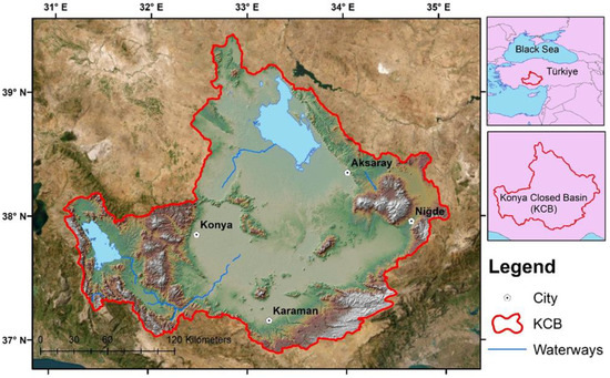
Figure 1.
Study area.
Konya, Turkey, is a significant region in terms of solar energy potential. The region receives an average annual solar radiation of 4.6–4.8 kWh/m2/day. This high solar energy potential provides favorable conditions for the development of integrated solar energy projects [58]. Turkey is planning integrated solar projects to increase solar energy production, and these projects aim to reduce CO2 emissions. The planned projects use two main technologies: solar power plants and photovoltaic systems. These projects aim to contribute to Turkey’s renewable energy targets by increasing the sustainable use of solar energy. Given these factors, Konya was selected as the study area due to its semi-arid climate, high solar radiation potential, and increasing interest in solar energy projects in the region.
2.2. Data Collection
In this study, climatic and meteorological data obtained from the NASA/POWER dataset were used. The study area is located within the boundaries of the Konya Closed Basin, with Konya province (37.8667° N, 32.4833° E) chosen as the reference point due to its suitability for human settlement and representativeness. According to the MERRA-2 dataset, the elevation of the region above sea level was calculated as 1215.57 m. The study utilized data covering the period from 1 January 1984 to 31 December 2022, with analyses conducted on a monthly scale. In the original dataset, solar radiation is represented by the ALLSKY_SFC_SW_DWN variable, which corresponds to all-sky surface shortwave downward radiation (kWh/m2/day). This variable represents radiation on a horizontal plane and includes both direct and diffuse radiation, making it suitable for assessing overall solar energy availability at the surface. Precipitation is represented by the PRECTOTCORR variable, which provides MERRA-2 corrected total precipitation data (mm/day). Relative humidity is denoted by the RH2M variable, representing the relative humidity (%) at a 2 m level according to MERRA-2. Air temperature is represented by the T2M variable, indicating the air temperature (°C) at a 2 m level based on MERRA-2 data. Wind speed is derived from the WS2M variable, which corresponds to the wind speed (m/s) at a 2 m level obtained from the MERRA-2 dataset. For more detailed information about the datasets, the following reference can be consulted [42]. The parameters examined in this study include solar radiation, precipitation, relative humidity, temperature, and wind speed. The variations of the datasets over time are presented in Figure 2.
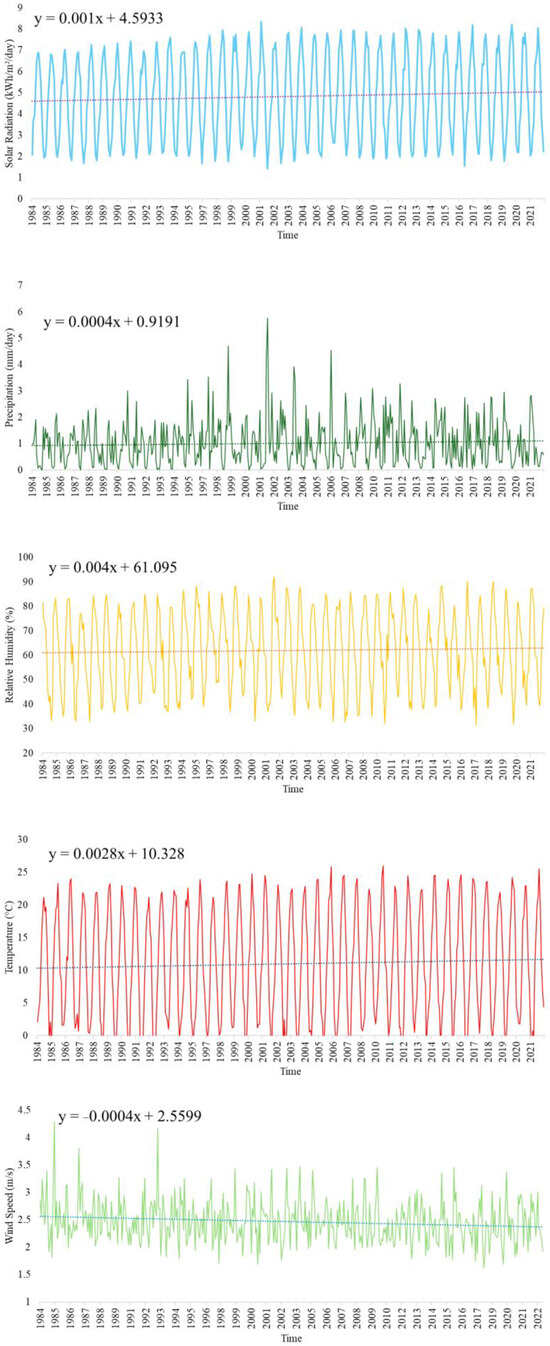
Figure 2.
Temporal variations of datasets.
These data were used to evaluate the climatic characteristics of the study area and analyze meteorological trends. Statistical information about the data is presented in Table 1.

Table 1.
Statistical information about the parameters.
In selecting these parameters, the correlation coefficient with the investigated solar radiation variable was considered in the estimation modeling. The graphic for visualizing the correlation coefficients is presented in Figure 3. This analysis contributes to the modeling process by determining the relationship between the climatic variables in the study area and solar radiation.
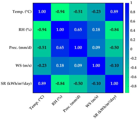
Figure 3.
The correlation coefficients of parameters.
In Figure 3, the color gradient represents the strength and direction of the correlation: darker blue tones indicate stronger positive correlations, while green tones represent weaker or negative correlations. Values range from −1 (strong negative correlation) to 1 (strong positive correlation).
2.3. Prediction Models
2.3.1. LSTM
Hochreiter and Schmidhuber [59], introduced the concept of long short-term memory networks, which are an artificial recurrent neural network (RNN) architecture utilized in the deep learning field [60]. Unlike standard feedforward neural networks, LSTM has feedback connections. LSTM consists of a memory cell that contains a forget gate (ft), an input gate (it), and an output gate (Ot) to control the flow of information. At each time step t, the hidden state ht is updated using the vector xt, the previous hidden state ht−1, and the previous cell state ct−1. Figure 4 depicts the fundamental design of the LSTM as well as its internal cell, or memory unit.
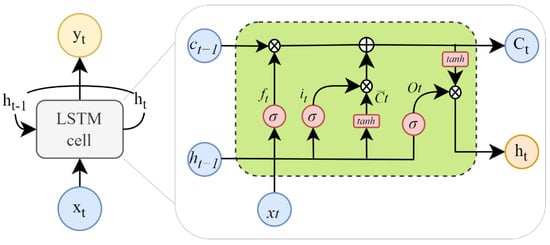
Figure 4.
The LSTM structure.
LSTM forward pass process along time steps can be expressed with vector formulas as follows [61]:
forget gate:
input gate:
output gate:
new value:
cell state:
hidden state:
Here, the parameters of the gates are the weights (Wi, Wf, Wc, Wo) and biases (bi, bf, bc, bo) that associate with the input (xt) and the previous hidden state (ht−1). is the candidate cell state passing through the input gate and range (−1, 1). Both the current state (Ct) and the prior state (Ct−1) of the memory cell exist. tanh is the hyperbolic tangent activation function, while σ is the sigmoid activation function. ⊗ stands for the convolutional operation (Hadamard product). The current state and the output gate determine the cell’s output (ht).
2.3.2. BiLSTM
Bidirectional Long Short-Term Memory (BiLSTM) neural network combines the information from the input sequence by processing it in both forward and backward directions [62]. This model consists of a forward LSTM and a backward LSTM, so the network can learn temporal dependencies in both directions [63]. The basic structure of BiLSTM is shown in Figure 5.
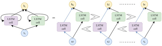
Figure 5.
The BiLSTM structure.
2.3.3. GRU
Gated Recurrent Units (GRU) is a simpler version of RNN that improves performance [64]. Like RNN and LSTM, GRU can be used to make time-series predictions. The GRU model structure, as illustrated in Figure 6, consists of only two gates: the reset gate rt and the update gate zt.
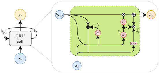
Figure 6.
The GRU structure.
The reset gate rt determines how much information from the new input xt and the previous state is retained in the current hidden layer vector . On the other hand, the update gate zt controls the preservation of the previous hidden state ht−1. Compared to LSTM, GRU’s fewer gates contribute to its higher efficiency [65]. The GRU transition functions are formulated as follows.
Here, the reset gate rt is defined by the weight matrices Wrx, Wrh, and the bias term br. Similarly, the update gate zt is determined by the weight matrices Wzx, Wzh, and the bias term bz. Additionally, bh represents the bias associated with the current hidden layer vector .
2.3.4. BiGRU
GRU is a type of unidirectional neural network structure. Unidirectional neural network models are feedforward, and the output is always taken from the previous layer. The Bidirectional Gated Recurrent Units (BiGRU) model is a combined version of the two-GRU architecture. In each case, the input provides two GRUs in the opposite direction and the output is determined by two unidirectional GRUs [66]. The identical conception and equations used for the normal GRU are also used for the forward and reversed GRUs [67]. The basic structure of BiGRU is shown in Figure 7.

Figure 7.
The BiGRU structure.
In deep learning techniques, weights are updated throughout training via optimization algorithms. Of these methods, the more stable and quicker Stochastic Gradient Descent with Momentum (SGD with Momentum) algorithm is compared to the simpler and slower Stochastic Gradient Descent (SGD) method. AdaGrad, or the adaptive gradient algorithm, performs well with sparse data, although its learning rate may eventually drop. For LSTMs, Root Mean Square Propagation (RMSProp) offers balanced learning, while the most used approach, Adaptive Moment Estimation (ADAM), is quick and reliable. AdaGrad is enhanced with Adaptive Delta (AdaDelta), while Nesterov Momentum offers accelerated and anticipatory momentum. In general, the most preferred algorithm is ADAM [31,63].
2.3.5. LSBoost
Least Squares Boosting minimizes errors by employing an ensemble approach made up of several weak learners. By training each weak learner to lower the error rates of earlier models, the total model can provide predictions that are increasingly correct. LSBoost performs remarkably well thanks to its adaptable structure, especially in noisy, irregular, and highly variable datasets. The random fluctuations and abrupt shifts frequently seen in time series data are especially well-handled by this model. By correcting the errors of previous models during the learning process, LSBoost increases overall prediction accuracy when working with highly variable datasets. Furthermore, it makes up for the shortcomings of previous models, enabling it to more accurately depict intricate relationships seen in the data. These features make LSBoost a very effective prediction tool, particularly for time series data with unpredictable, seasonal, or irregular changes [68].
2.3.6. XGBoost
XGBoost introduces a new paradigm by optimizing decision tree algorithms to enhance database processing [52]. In this method, different types of regularization terms can be selected to reduce the risk of overfitting. Additionally, parallel computation is automatically applied during training to improve computational efficiency. Furthermore, the functions within the XGBoost model are executed and calculated automatically during the training phase. The XGBoost model consists of n decision trees. Each tree considers the residuals of the previous tree and utilizes a gradient algorithm to construct new decision trees. As a result, the residual errors during the training process are minimized. The previous predictors are redeveloped in each iteration to further reduce residual errors [69].
2.3.7. Bagging
Bootstrap aggregation, often known as bagging, is a process that involves periodically sampling a data collection and replacing it with a uniform probability distribution [70]. It is frequently referred to as a collection of homogenous weak learners who study independently in parallel and then integrate their knowledge using a deterministic averaging technique [71].
2.3.8. Random Forest
The Random Forest method is a widely used ensemble learning technique for regression. Ho [72] proposed the Random Forest approach based on the random subspace method, aiming to generate multiple decision trees with controlled variance to improve accuracy and mitigate overfitting issues during training. RF consists of an ensemble of independent decision trees and randomly selected data samples. To build a model, typically, two-thirds of the dataset is used to construct decision trees, while the remaining portion is reserved for evaluating the model’s accuracy, error rate, and overall performance. In the next step, the results from all generated decision trees are aggregated, and the best-performing model is identified based on the majority vote of all trees [73].
2.3.9. SVM
Support vector machines (SVMs) are a machine learning methodology designed for executing both classification and regression tasks, developed by Vapnik [74]. The theoretical basis of SVM is grounded in statistical learning theory and the concept of structural risk reduction [75]. A regression model known as support vector machine regression (SVMR) was developed by Smola. SVR models combine regression functions with an SVM to solve regression, prediction, and forecasting problems [76,77]. The input-output dataset for SVR is represented as (x,y) [78], where x is the input vector and y denotes the output vector. The summary of the SVR regression function is as follows:
where the coefficients βi and βi* are interpreted as forces that push and pull the regression estimate f(x) toward the measurements. A bias term and a weight vector are denoted by w and b. The structure of the SVM model is shown in Figure 8.
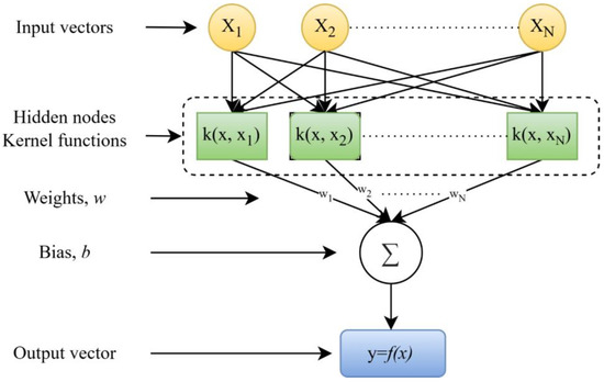
Figure 8.
The SVR structure.
The optimal outcomes in SVMR are attained through the use of Lagrangian multipliers and kernel functions. Different kernel functions, such as linear, polynomial, radial basis function (RBF), and sigmoid, are utilized in SVMR, and the role of kernels gives SVM the ability to model complex separating hyperplanes [77,79].
2.3.10. GRNN
The GRNN has four layers: input, pattern, summation, and output (Figure 9). The total number of parameters is the same as the number of input units in the first layer. The first layer is completely related to the second layer, the pattern layer. Each unit in the pattern layer represents a training pattern, and its output is the input’s distance from the stored patterns. The output layer divides the output of each S-summation neuron by the output of each D-summation neuron to obtain the anticipated value for an unknown input vector x. For further details, please see the given reference [80].
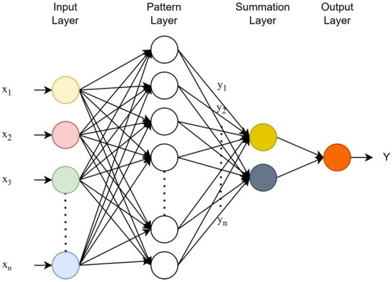
Figure 9.
The GRANN structure.
2.3.11. MANN
MLANN consists of an input layer, one or more hidden (intermediate) layers, and an output layer where data are received as input. MLANN contains forward and backward propagation, which are layer transitions. Throughout the forward propagation phase, the output and error values of the network are computed. The estimated error value is minimized during the backward propagation phase by updating the inter-layer connection weights [81]. Neurons in the input layer of the MANN model process incoming data. Consequently, the number of input values in the dataset and the number of neurons in the input layer must match. The input values are sent directly from the input layer’s neurons to the hidden layer. The total value is determined by each neuron in the hidden layer by adding the threshold value to the weighted input values. It is then processed using an activation function and sent either straight to the output layer or to the next layer. At the beginning, the weights between layers are often chosen at random. By contrasting the network’s output values with the anticipated output values, the error value is determined [82].
2.3.12. RBANN
Broomhead and Lowe first presented the idea of RBANN in the literature in 1988 [83]. The stimulus–response states of neuron cells in the human nervous system were taken into consideration when developing the ANN model and radial-based functionalities. Like the MLANN structure, the RBANN structure typically comprises an input layer, a hidden layer, and an output layer [84]. In contrast to other MLANN types, nonlinear clustering analysis and radial-based activation functions are applied to the data as it moves from the input layer to the hidden layer. The real training process occurs in this layer, and the structure between the hidden layer and the output layer operates similarly to other ANN types [85].
2.4. Metrics for Performance Evaluation of Models
Three fundamental statistical criteria were applied in this study with the aim of choosing the best model. Among these criteria are the mean absolute error (MAE) (m³/s), which calculates the average difference between the predicted and actual values; the root mean square error (RMSE) (m³/s), which is commonly used in many iterative prediction and optimization methods; and the coefficient of determination (R2), a measure of the degree of association between the predicted and observed values. These criteria were used to evaluate the recommended hybrid models’ performance, and the resulting equations are shown below (Table 2).
Table 2.
Performance evaluation criteria.
Where SRm is the solar radiation variables measured; SRp is the solar radiation variables predicted by approaches; is the average of the predicted solar radiation variables, is the average of solar radiation variables; n is amount of data. In this study, scatter plots, Taylor diagrams, and violin diagrams were utilized as tools to compare the different approaches. These graphic approaches give an in-depth overview of how well the models match the observed data, providing important information about their accuracy and performance. Additionally, as part of the performance evaluation criteria, the Kruskal–Wallis test was used to evaluate the model distributions’ appropriateness [86,87,88].
3. Results
To illustrate the overall structure of the study framework in detail, a workflow diagram has been prepared. Verified data obtained from the NASA/POWER database using remote sensing techniques have been used to create datasets for prediction models based on high correlation relationships. The dataset was divided into 75% training and 25% testing to ensure sufficient learning while maintaining a robust evaluation set. Well-known successful methods, ranging from ANN algorithms to deep learning architectures in line with the progression in the literature, have been utilized with various optimization techniques to compare performance within the study. To prevent overfitting, model parameters and hyperparameters were selected based on insights from previous studies. Additionally, techniques such as early stopping and dropout regularization were applied to improve generalization and ensure robust model performance [31,42]. The hyper-parameters of the models are given in Table 3. The workflow diagram of the study is presented below (Figure 10).
Table 3.
Hyperparameters of models.
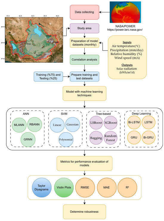
Figure 10.
The workflow diagram of the study.
The performance criteria for the training and testing phases are presented in Table 4 below. All error metrics (RMSE, MAE) are expressed in kWh/m2/day. In the table where the ranking is based on the test phase, the RMSE criterion has been considered.
Table 4.
Comparison of model results and success ranking.
Table 4 compares the performance of different machine learning models during the training and testing phases. In the training phase, the top three models with the best performance were LSBoost, Bi-LSTM, and GRU, respectively. During the testing phase, the best-performing models were the deep learning architectures LSTM, Bi-LSTM, and GRU, respectively. The LSTM model achieved the highest accuracy in the test phase with RMSE = 0.34, MAE = 0.27, and R2 = 0.97. Similarly, the Bi-LSTM model demonstrated strong performance with RMSE = 0.37, MAE = 0.31, and R2 = 0.97. These results highlight the strong predictive capability of deep learning models, especially for time series data. The GRU model also exhibited a balanced performance, ranking third with RMSE = 0.41, MAE = 0.33, and R2 = 0.97. A ranked comparison of the models based on their performance is presented in Figure 11.
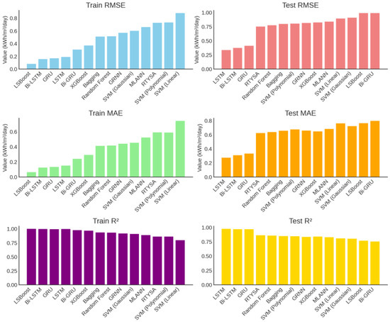
Figure 11.
Model performance comparison.
When examining Figure 11, it can be observed that during the training phase (Train RMSE, MAE, R2), the LSBoost, Bi-GRU, and LSTM models have the lowest RMSE and MAE values while demonstrating the highest R2 values, indicating that they achieved very effective learning on the training data. However, in the testing phase (Test RMSE, MAE, R2), the error rate of LSBoost increased significantly, and a decline in generalization performance was observed, which is an indication of overfitting. The LSTM, Bi-LSTM, and GRU models exhibited the best performance during the test phase, maintaining the lowest error rates and the highest R2 values. Among classical machine learning methods, XGBoost, Random Forest, and Bagging demonstrated balanced performance, whereas the SVM (Linear) and SVM (Gaussian) models showed the lowest performance with higher error rates and lower R2 values in both training and testing phases. The scatter plots of the models during the test phase are presented in Figure 12.
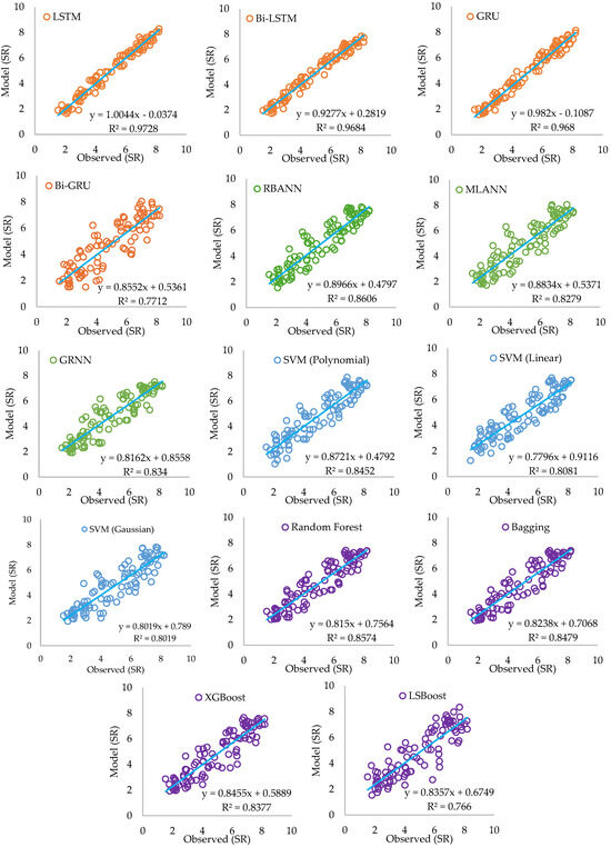
Figure 12.
Scatter plots of the models in the test phase.
4. Discussion
In this study, in addition to the low error values obtained from the prediction models, ANOVA and Kruskal–Wallis tests were applied to evaluate the robustness and generalization ability of the models. These tests were used to assess the compatibility between the model distributions and the observed data, as well as to determine whether they belong to the same population. The p-values for the Kruskal–Wallis and ANOVA tests are presented in Table 5.
Table 5.
The p-values of the Kruskal–Wallis and ANOVA tests.
The statistical analysis of the models using both the Kruskal–Wallis and ANOVA tests indicates that there is no significant difference between the observed values and the predictions made by each model. The p-values for all models in both tests are greater than 0.05, meaning that the distributions and means of the model predictions do not significantly deviate from the actual observed data. This suggests that all models perform similarly and can be considered statistically valid approximations of the observed values.
Although the LSBoost model achieved the lowest error rate (RMSE = 0.08, MAE = 0.06) and the highest R2 value (0.998) during the training phase, it was observed that its error rate increased significantly in the testing phase (RMSE = 0.99, MAE = 0.76, R2 = 0.77). This indicates that the model overfitted the training data, preventing it from generalizing effectively to the test data. This issue is also evident in the scatter plots presented in Figure 12. Similarly, models such as Bi-GRU and LSBoost, despite exhibiting very high performance during training, experienced a significant decline in performance during testing. This suggests that these models focused excessively on the training set, leading to poor generalization on unseen test data. Among the models, the XGBoost algorithm demonstrated moderate performance, achieving RMSE = 0.82 and R2 = 0.84. Among classical machine learning models, Random Forest and Bagging performed relatively well with R2 values of 0.86 and 0.85, respectively. However, their accuracy remained lower than that of LSTM and Bi-LSTM. Finally, SVM (Linear) and SVM (Gaussian) exhibited the lowest performance, achieving R2 values of 0.81 and 0.80 during the test phase, indicating lower accuracy compared to other models. These findings suggest that Support Vector Machines (SVMs) may not be well-suited for large datasets and complex time series data. Overall, while LSTM and Bi-LSTM models provided the best performance in the testing phase, models such as LSBoost and Bi-GRU failed to maintain their success due to overfitting, leading to reduced generalization capability on the test set. These results highlight the importance of selecting appropriate models based on dataset characteristics and forecasting objectives. In this context, the differences in model performance can be attributed to the intrinsic characteristics of each algorithm and the nature of the dataset. Deep learning models (LSTM, Bi-LSTM, and GRU) demonstrated superior accuracy due to their ability to capture temporal dependencies and nonlinear patterns in the data. Traditional machine learning models, such as Random Forest and XGBoost, provided robust performance but were slightly less effective in capturing sequential dependencies. Additionally, factors such as data periods, noise, and cloud cover variations can impact solar radiation forecasting [89,90]. Deep learning models, particularly LSTM-based architectures, have shown resilience against missing or noisy data by leveraging long-term dependencies. However, classical models, like SVM and simple regression methods (test: RMSE: 0.87, MAE: 0.76, R2: 0.81), struggled with these variations, leading to lower accuracy. Future studies could integrate data imputation techniques and hybrid models to further improve predictive performance in scenarios with incomplete data.
Although this study focused on meteorological parameters such as temperature, precipitation, relative humidity, and wind speed in solar radiation modeling, it is well known that aerosols and cloud droplets significantly affect radiation absorption and scattering. Aerosols change the solar energy availability at the surface by affecting shortwave and longwave radiation [91]. However, due to the clear sky conditions in the study region and the limitations of available aerosol data, they could not be included as primary variables in this analysis. Future studies can integrate aerosols to further improve solar radiation prediction models. While this study primarily focuses on machine learning-based prediction, it is essential to recognize that general atmospheric circulation models also play a significant role in dynamic solar radiation prediction through numerical simulations. These models, which account for large-scale atmospheric processes, can produce short-term solar radiation estimates. However, their high computational demands and complexity often necessitate the use of data-driven approaches, such as machine learning, to enhance efficiency and improve localized predictions [23].
5. Conclusions
This study compares the performance of various machine learning models for solar radiation prediction in the Konya region. The results revealed that deep learning models, particularly LSTM (RMSE = 0.34, MAE = 0.27, R2 = 0.97) and Bi-LSTM (RMSE = 0.37, MAE = 0.31, R2 = 0.97), had the lowest error rates and the highest accuracy. The GRU model (RMSE = 0.41, MAE = 0.33, R2 = 0.97) also demonstrated strong predictive capability, ranking third in performance. Although LSBoost achieved low error rates in the training phase (RMSE = 0.08, MAE = 0.06, R2 = 0.998), its performance significantly declined in the testing phase (RMSE = 0.99, MAE = 0.76, R2 = 0.77), indicating overfitting. Similarly, the Bi-GRU model (RMSE = 0.99, MAE = 0.80, R2 = 0.75) also exhibited reduced generalization performance in the test phase. Among Boost and tree-based approaches, XGBoost (RMSE = 0.82, MAE = 0.65, R2 = 0.84), Random Forest (RMSE = 0.77, MAE = 0.64, R2 = 0.86), and Bagging (RMSE = 0.80, MAE = 0.66, R2 = 0.85) provided balanced performance. However, SVM (Linear: RMSE = 0.89, R2 = 0.81; Gaussian: RMSE = 0.91, R2 = 0.80) models had relatively lower accuracy in solar radiation prediction. The results indicate that LSTM and Bi-LSTM outperform other models due to their superior ability to capture temporal dependencies in solar radiation data. The study also highlights that traditional machine learning models, such as Random Forest and XGBoost, perform well but are slightly limited in sequential learning.
Statistical analyses (ANOVA and Kruskal–Wallis tests) indicated no significant difference between the predicted and observed values (p > 0.05), confirming the reliability of the models. Overall, LSTM and Bi-LSTM were identified as the best-performing models, while LSBoost and Bi-GRU suffered from overfitting, leading to poor generalization on the test data. Future studies should explore larger datasets, alternative optimization techniques, and hybrid model approaches to further enhance prediction accuracy.
Funding
This research received no external funding.
Institutional Review Board Statement
Not applicable.
Informed Consent Statement
Not applicable.
Data Availability Statement
The data supporting the findings of this study are available from the corresponding author upon reasonable request.
Acknowledgments
The author would like to thank the NASA POWER team for their significant contributions in providing the data used in this study.
Conflicts of Interest
The author declares no conflicts of interest.
References
- Albergel, C.; Dutra, E.; Munier, S.; Calvet, J.-C.; Munoz-Sabater, J.; de Rosnay, P.; Balsamo, G. ERA-5 and ERA-Interim Driven ISBA Land Surface Model Simulations: Which One Performs Better? Hydrol. Earth Syst. Sci. 2018, 22, 3515–3532. [Google Scholar] [CrossRef]
- Khamees, A.S.; Sayad, T.; Morsy, M.; Ali Rahoma, U. Evaluation of Three Radiation Schemes of the WRF-Solar Model for Global Surface Solar Radiation Forecast: A Case Study in Egypt. Adv. Space Res. 2024, 73, 2880–2891. [Google Scholar] [CrossRef]
- Gao, X.-J.; Shi, Y.; Giorgi, F. Comparison of Convective Parameterizations in RegCM4 Experiments over China with CLM as the Land Surface Model. Atmos. Ocean. Sci. Lett. 2016, 9, 246–254. [Google Scholar] [CrossRef]
- Lockwood, J.G. Atmospheric Circulation, Global. In Climatology Encyclopedia of Earth Science; Springer: Boston, MA, USA, 1987; pp. 131–140. [Google Scholar]
- Krishnan, N.; Kumar, K.R.; Inda, C.S. How Solar Radiation Forecasting Impacts the Utilization of Solar Energy: A Critical Review. J. Clean. Prod. 2023, 388, 135860. [Google Scholar] [CrossRef]
- Kumler, A.; Kravitz, B.; Draxl, C.; Vimmerstedt, L.; Benton, B.; Lundquist, J.K.; Martin, M.; Buck, H.J.; Wang, H.; Lennard, C.; et al. Potential Effects of Climate Change and Solar Radiation Modification on Renewable Energy Resources. Renew. Sustain. Energy Rev. 2025, 207, 114934. [Google Scholar] [CrossRef]
- Abdallah, M.; Mohammadi, B.; Nasiri, H.; Katipoğlu, O.M.; Abdalla, M.A.A.; Ebadzadeh, M.M. Daily Global Solar Radiation Time Series Prediction Using Variational Mode Decomposition Combined with Multi-Functional Recurrent Fuzzy Neural Network and Quantile Regression Forests Algorithm. Energy Rep. 2023, 10, 4198–4217. [Google Scholar] [CrossRef]
- Huang, J.; Jing, L.; Zhang, Q.; Zong, S.; Zhang, A. Interfacial Solar Vapor Evaporator Based on Biologically Natural Composites. Nano Energy 2025, 133, 110458. [Google Scholar] [CrossRef]
- Mehdizadeh, S.; Mohammadi, B.; Pham, Q.B.; Duan, Z. Development of Boosted Machine Learning Models for Estimating Daily Reference Evapotranspiration and Comparison with Empirical Approaches. Water 2021, 13, 3489. [Google Scholar] [CrossRef]
- Mohammadi, B.; Moazenzadeh, R. Performance Analysis of Daily Global Solar Radiation Models in Peru by Regression Analysis. Atmosphere 2021, 12, 389. [Google Scholar] [CrossRef]
- Mohanty, S.; Patra, P.K.; Sahoo, S.S. Prediction and Application of Solar Radiation with Soft Computing over Traditional and Conventional Approach—A Comprehensive Review. Renew. Sustain. Energy Rev. 2016, 56, 778–796. [Google Scholar] [CrossRef]
- Qin, S.; Liu, Z.; Qiu, R.; Luo, Y.; Wu, J.; Zhang, B.; Wu, L.; Agathokleous, E. Short–Term Global Solar Radiation Forecasting Based on an Improved Method for Sunshine Duration Prediction and Public Weather Forecasts. Appl. Energy 2023, 343, 121205. [Google Scholar] [CrossRef]
- Almorox, J.; Hontoria, C. Global Solar Radiation Estimation Using Sunshine Duration in Spain. Energy Convers. Manag. 2004, 45, 1529–1535. [Google Scholar] [CrossRef]
- Duzen, H.; Aydin, H. Sunshine-Based Estimation of Global Solar Radiation on Horizontal Surface at Lake Van Region (Turkey). Energy Convers. Manag. 2012, 58, 35–46. [Google Scholar] [CrossRef]
- Almorox, J.; Bocco, M.; Willington, E. Estimation of Daily Global Solar Radiation from Measured Temperatures at Cañada de Luque, Córdoba, Argentina. Renew. Energy 2013, 60, 382–387. [Google Scholar] [CrossRef]
- Fan, J.; Chen, B.; Wu, L.; Zhang, F.; Lu, X.; Xiang, Y. Evaluation and Development of Temperature-Based Empirical Models for Estimating Daily Global Solar Radiation in Humid Regions. Energy 2018, 144, 903–914. [Google Scholar] [CrossRef]
- Gu, L.; Fuentes, J.D.; Garstang, M.; Da Silva, J.T.; Heitz, R.; Sigler, J.; Shugart, H.H. Cloud Modulation of Surface Solar Irradiance at a Pasture Site in Southern Brazil. Agric. For. Meteorol. 2001, 106, 117–129. [Google Scholar] [CrossRef]
- Kostić, R.; Mikulović, J. The Empirical Models for Estimating Solar Insolation in Serbia by Using Meteorological Data on Cloudiness. Renew. Energy 2017, 114, 1281–1293. [Google Scholar] [CrossRef]
- Chen, J.-L.; He, L.; Yang, H.; Ma, M.; Chen, Q.; Wu, S.-J.; Xiao, Z. Empirical Models for Estimating Monthly Global Solar Radiation: A Most Comprehensive Review and Comparative Case Study in China. Renew. Sustain. Energy Rev. 2019, 108, 91–111. [Google Scholar] [CrossRef]
- Fan, J.; Wang, X.; Wu, L.; Zhang, F.; Bai, H.; Lu, X.; Xiang, Y. New Combined Models for Estimating Daily Global Solar Radiation Based on Sunshine Duration in Humid Regions: A Case Study in South China. Energy Convers. Manag. 2018, 156, 618–625. [Google Scholar] [CrossRef]
- Qiu, R.; Liu, C.; Cui, N.; Gao, Y.; Li, L.; Wu, Z.; Jiang, S.; Hu, M. Generalized Extreme Gradient Boosting Model for Predicting Daily Global Solar Radiation for Locations without Historical Data. Energy Convers. Manag. 2022, 258, 115488. [Google Scholar] [CrossRef]
- Feng, Y.; Gong, D.; Zhang, Q.; Jiang, S.; Zhao, L.; Cui, N. Evaluation of Temperature-Based Machine Learning and Empirical Models for Predicting Daily Global Solar Radiation. Energy Convers. Manag. 2019, 198, 111780. [Google Scholar] [CrossRef]
- Kurgansky, M.V.; Krupchatnikov, V.N. Dynamic Meteorology. Russ. Natl. Rep. Meteorol. Atmos. 2019, 152. [Google Scholar]
- Hammer, A.; Heinemann, D.; Lorenz, E.; Lückehe, B. Short-Term Forecasting of Solar Radiation: A Statistical Approach Using Satellite Data. Sol. Energy 1999, 67, 139–150. [Google Scholar] [CrossRef]
- Lorenz, E.; Hammer, A.; Heienmann, D. Short Term Forecasting of Solar Radiation Based on Cloud Motion Vectors from Satellite Images. ISES Eur. Sol. Congr. 2004, 1, 841–848. [Google Scholar]
- White, J.W.; Hoogenboom, G.; Wilkens, P.W.; Stackhouse, P.W.; Hoel, J.M. Evaluation of Satellite-Based, Modeled-Derived Daily Solar Radiation Data for the Continental United States. Agron. J. 2011, 103, 1242–1251. [Google Scholar] [CrossRef]
- Qing, X.; Niu, Y. Hourly Day-Ahead Solar Irradiance Prediction Using Weather Forecasts by LSTM. Energy 2018, 148, 461–468. [Google Scholar] [CrossRef]
- Sharda, S.; Singh, M.; Sharma, K. RSAM: Robust Self-Attention Based Multi-Horizon Model for Solar Irradiance Forecasting. IEEE Trans. Sustain. Energy 2021, 12, 1394–1405. [Google Scholar] [CrossRef]
- Hassan, M.A.; Khalil, A.; Kaseb, S.; Kassem, M.A. Exploring the Potential of Tree-Based Ensemble Methods in Solar Radiation Modeling. Appl. Energy 2017, 203, 897–916. [Google Scholar] [CrossRef]
- Notton, G.; Voyant, C.; Fouilloy, A.; Duchaud, J.L.; Nivet, M.L. Some Applications of ANN to Solar Radiation Estimation and Forecasting for Energy Applications. Appl. Sci. 2019, 9, 209. [Google Scholar] [CrossRef]
- Demir, V.; Citakoglu, H. Forecasting of Solar Radiation Using Different Machine Learning Approaches. Neural Comput. Appl. 2023, 35, 887–906. [Google Scholar] [CrossRef]
- Demirgül, T.; Demir, V.; Sevimli, M.F. Forecasting of HELIOSAT-Based Solar Radiation by Model-Tree (M5-Tree) Approach. Geomatik 2023, 8, 124–135. [Google Scholar] [CrossRef]
- Jiang, C.; Zhu, Q. Evaluating the Most Significant Input Parameters for Forecasting Global Solar Radiation of Different Sequences Based on Informer. Appl. Energy 2023, 348, 121544. [Google Scholar] [CrossRef]
- Neshat, M.; Nezhad, M.M.; Mirjalili, S.; Garcia, D.A.; Dahlquist, E.; Gandomi, A.H. Short-Term Solar Radiation Forecasting Using Hybrid Deep Residual Learning and Gated LSTM Recurrent Network with Differential Covariance Matrix Adaptation Evolution Strategy. Energy 2023, 278, 127701. [Google Scholar] [CrossRef]
- Marinho, F.P.; Rocha, P.A.C.; Neto, A.R.R.; Bezerra, F.D.V. Short-Term Solar Irradiance Forecasting Using CNN-1D, LSTM, and CNN-LSTM Deep Neural Networks: A Case Study With the Folsom (USA) Dataset. J. Sol. Energy Eng. 2023, 145, 041002. [Google Scholar] [CrossRef]
- Ehteram, M.; Afshari Nia, M.; Panahi, F.; Farrokhi, A. Read-First LSTM Model: A New Variant of Long Short Term Memory Neural Network for Predicting Solar Radiation Data. Energy Convers. Manag. 2024, 305, 118267. [Google Scholar] [CrossRef]
- Zhang, C.; Zhang, Y.; Pu, J.; Liu, Z.; Wang, Z.; Wang, L. An Hourly Solar Radiation Prediction Model Using EXtreme Gradient Boosting Algorithm with the Effect of Fog-Haze. Energy Built Environ. 2025, 6, 18–26. [Google Scholar] [CrossRef]
- Solano, E.S.; Dehghanian, P.; Affonso, C.M. Solar Radiation Forecasting Using Machine Learning and Ensemble Feature Selection. Energies 2022, 15, 7049. [Google Scholar] [CrossRef]
- Huang, L.; Kang, J.; Wan, M.; Fang, L.; Zhang, C.; Zeng, Z. Solar Radiation Prediction Using Different Machine Learning Algorithms and Implications for Extreme Climate Events. Front. Earth Sci. 2021, 9, 596860. [Google Scholar] [CrossRef]
- Abumohsen, M.; Owda, A.Y.; Owda, M.; Abumihsan, A. Hybrid Machine Learning Model Combining of CNN-LSTM-RF for Time Series Forecasting of Solar Power Generation. Adv. Electr. Eng. Electron. Energy 2024, 9, 100636. [Google Scholar] [CrossRef]
- Perez-Rodriguez, S.A.; Alvarez-Alvarado, J.M.; Romero-Gonzalez, J.A.; Aviles, M.; Mendoza-Rojas, A.E.; Fuentes-Silva, C.; Rodriguez-Resendiz, J. Metaheuristic Algorithms for Solar Radiation Prediction: A Systematic Analysis. IEEE Access 2024, 12, 100134–100151. [Google Scholar] [CrossRef]
- Mendyl, A.; Demir, V.; Omar, N.; Orhan, O.; Weidinger, T. Enhancing Solar Radiation Forecasting in Diverse Moroccan Climate Zones: A Comparative Study of Machine Learning Models with Sugeno Integral Aggregation. Atmosphere 2024, 15, 103. [Google Scholar] [CrossRef]
- Mirbolouki, A.; Heddam, S.; Singh Parmar, K.; Trajkovic, S.; Mehraein, M.; Kisi, O. Comparison of the Advanced Machine Learning Methods for Better Prediction Accuracy of Solar Radiation Using Only Temperature Data: A Case Study. Int. J. Energy Res. 2022, 46, 2709–2736. [Google Scholar] [CrossRef]
- Hissou, H.; Benkirane, S.; Guezzaz, A.; Azrour, M.; Beni-Hssane, A. A Novel Machine Learning Approach for Solar Radiation Estimation. Sustainability 2023, 15, 10609. [Google Scholar] [CrossRef]
- Kisi, O.; Parmar, K.S. Application of Least Square Support Vector Machine and Multivariate Adaptive Regression Spline Models in Long Term Prediction of River Water Pollution. J. Hydrol. 2016, 534, 104–112. [Google Scholar] [CrossRef]
- Alizamir, M.; Othman Ahmed, K.; Shiri, J.; Fakheri Fard, A.; Kim, S.; Heddam, S.; Kisi, O. A New Insight for Daily Solar Radiation Prediction by Meteorological Data Using an Advanced Artificial Intelligence Algorithm: Deep Extreme Learning Machine Integrated with Variational Mode Decomposition Technique. Sustainability 2023, 15, 11275. [Google Scholar] [CrossRef]
- Alizamir, M.; Shiri, J.; Fard, A.F.; Kim, S.; Gorgij, A.D.; Heddam, S.; Singh, V.P. Improving the Accuracy of Daily Solar Radiation Prediction by Climatic Data Using an Efficient Hybrid Deep Learning Model: Long Short-Term Memory (LSTM) Network Coupled with Wavelet Transform. Eng. Appl. Artif. Intell. 2023, 123, 106199. [Google Scholar] [CrossRef]
- Hussain, S.; AlAlili, A. A Hybrid Solar Radiation Modeling Approach Using Wavelet Multiresolution Analysis and Artificial Neural Networks. Appl. Energy 2017, 208, 540–550. [Google Scholar] [CrossRef]
- Qiu, R.; Li, L.; Wu, L.; Agathokleous, E.; Liu, C.; Zhang, B.; Luo, Y.; Sun, S. Modeling Daily Global Solar Radiation Using Only Temperature Data: Past, Development, and Future. Renew. Sustain. Energy Rev. 2022, 163, 112511. [Google Scholar] [CrossRef]
- Voyant, C.; Notton, G.; Kalogirou, S.; Nivet, M.-L.; Paoli, C.; Motte, F.; Fouilloy, A. Machine Learning Methods for Solar Radiation Forecasting: A Review. Renew. Energy 2017, 105, 569–582. [Google Scholar] [CrossRef]
- Pedro, H.T.C.; Coimbra, C.F.M.; David, M.; Lauret, P. Assessment of Machine Learning Techniques for Deterministic and Probabilistic Intra-Hour Solar Forecasts. Renew. Energy 2018, 123, 191–203. [Google Scholar] [CrossRef]
- Chen, T.; Guestrin, C. XGBoost: A Scalable Tree Boosting System. In Proceedings of the 22nd ACM Sigkdd International Conference on Knowledge Discovery and Data Mining, San Francisco, CA, USA, 13–17 August 2016; pp. 785–794. [Google Scholar] [CrossRef]
- Fan, J.; Wang, X.; Wu, L.; Zhou, H.; Zhang, F.; Yu, X.; Lu, X.; Xiang, Y. Comparison of Support Vector Machine and Extreme Gradient Boosting for Predicting Daily Global Solar Radiation Using Temperature and Precipitation in Humid Subtropical Climates: A Case Study in China. Energy Convers. Manag. 2018, 164, 102–111. [Google Scholar] [CrossRef]
- Alam, M.S.; Al-Ismail, F.S.; Hossain, M.S.; Rahman, S.M. Ensemble Machine-Learning Models for Accurate Prediction of Solar Irradiation in Bangladesh. Processes 2023, 11, 908. [Google Scholar] [CrossRef]
- Krishnan, N.; Ravi Kumar, K. Solar Radiation Forecasting Using Gradient Boosting Based Ensemble Learning Model for Various Climatic Zones. Sustain. Energy Grids Networks 2024, 38, 101312. [Google Scholar] [CrossRef]
- Orhan, O.; Yakar, M.; Ekercin, S. An Application on Sinkhole Susceptibility Mapping by Integrating Remote Sensing and Geographic Information Systems. Arab. J. Geosci. 2020, 13, 886. [Google Scholar] [CrossRef]
- Demir, V.; Keskin, A.Ü. Water Level Change of Lakes and Sinkholes in Central Turkey under Anthropogenic Effects. Theor. Appl. Climatol. 2020, 142, 929–943. [Google Scholar] [CrossRef]
- General Directorate of Meteorology Türkiye Global Solar Radiation Long-Year Average (2004–2021) Heliosat Model Products. Available online: https://www.mgm.gov.tr/kurumici/radyasyon_iller.aspx?il=konya (accessed on 1 January 2025).
- Hochreiter, S.; Schmidhuber, J. Long Short-Term Memory. Neural Comput. 1997, 9, 1735–1780. [Google Scholar] [CrossRef] [PubMed]
- Xu, L.; Shi, P.; Wu, H.; Qu, S.; Li, Q.; Sun, Y.; Yang, X.; Jiang, P.; Qiu, C. Investigating the Potential of EMA-Embedded Feature Selection Method for ESVR and LSTM to Enhance the Robustness of Monthly Streamflow Forecasting from Local Meteorological Information. J. Hydrol. 2024, 636, 131230. [Google Scholar] [CrossRef]
- Wang, H.; Zhang, J.; Yang, J. Time Series Forecasting of Pedestrian-Level Urban Air Temperature by LSTM: Guidance for Practitioners. Urban Clim. 2024, 56, 102063. [Google Scholar] [CrossRef]
- Hou, Z.; Wang, B.; Zhang, Y.; Zhang, J.; Song, J. Drought Prediction in Jilin Province Based on Deep Learning and Spatio-Temporal Sequence Modeling. J. Hydrol. 2024, 642, 131891. [Google Scholar] [CrossRef]
- Wang, T.; Tu, X.; Singh, V.P.; Chen, X.; Lin, K.; Zhou, Z. Drought Prediction: Insights from the Fusion of LSTM and Multi-Source Factors. Sci. Total Environ. 2023, 902, 166361. [Google Scholar] [CrossRef]
- Zhao, R.; Wang, D.; Yan, R.; Mao, K.; Shen, F.; Wang, J. Machine Health Monitoring Using Local Feature-Based Gated Recurrent Unit Networks. IEEE Trans. Ind. Electron. 2018, 65, 1539–1548. [Google Scholar] [CrossRef]
- Zhang, W.; Li, H.; Tang, L.; Gu, X.; Wang, L.; Wang, L. Displacement Prediction of Jiuxianping Landslide Using Gated Recurrent Unit (GRU) Networks. Acta Geotech. 2022, 17, 1367–1382. [Google Scholar] [CrossRef]
- Anki, P.; Bustamam, A.; Buyung, R.A. Comparative Analysis of Performance between Multimodal Implementation of Chatbot Based on News Classification Data Using Categories. Electronics 2021, 10, 2696. [Google Scholar] [CrossRef]
- Aloraifan, D.; Ahmad, I.; Alrashed, E. Deep Learning Based Network Traffic Matrix Prediction. Int. J. Intell. Networks 2021, 2, 46–56. [Google Scholar] [CrossRef]
- Küllahcı, K.; Altunkaynak, A. Eigen Time Series Modeling: A Breakthrough Approach to Spatio-Temporal Rainfall Forecasting in Basins. Neural Comput. Appl. 2024, 37, 4471–4492. [Google Scholar] [CrossRef]
- Dong, J.; Zeng, W.; Wu, L.; Huang, J.; Gaiser, T.; Srivastava, A.K. Enhancing Short-Term Forecasting of Daily Precipitation Using Numerical Weather Prediction Bias Correcting with XGBoost in Different Regions of China. Eng. Appl. Artif. Intell. 2023, 117, 105579. [Google Scholar] [CrossRef]
- Bushara, N.O.; Abraham, A. Novel Ensemble Method for Long Term Rainfall Prediction. Int. J. Comput. Inf. Syst. Ind. Manag. Appl. 2015, 7, 116–130. [Google Scholar]
- Kundu, S.; Biswas, S.K.; Tripathi, D.; Karmakar, R.; Majumdar, S.; Mandal, S. A Review on Rainfall Forecasting Using Ensemble Learning Techniques. e-Prime—Adv. Electr. Eng. Electron. Energy 2023, 6, 100296. [Google Scholar] [CrossRef]
- Ho, T.K. Random Decision Forests. In Proceedings of the Proceedings of 3rd International Conference on Document Analysis And Recognition, Montreal, QC, Canada, 14–16 August 1995; IEEE: Piscataway, NJ, USA, 1995; Volume 1, pp. 278–282. [Google Scholar]
- Mosavi, A.; Sajedi Hosseini, F.; Choubin, B.; Goodarzi, M.; Dineva, A.A.; Rafiei Sardooi, E. Ensemble Boosting and Bagging Based Machine Learning Models for Groundwater Potential Prediction. Water Resour. Manag. 2021, 35, 23–37. [Google Scholar] [CrossRef]
- Vapnik, V. The Nature of Statistical Learning Theory; Springer: New York, NY, USA, 1995. [Google Scholar]
- Cortes, C.; Vapnik, V. Support-Vector Networks. Mach. Learn. 1995, 20, 273–297. [Google Scholar] [CrossRef]
- Smola, A. Regression Estimation with Support Vector Learning Machines. Master’s Thesis, Tech Univ Munchen, Munich, Germany, 1996. [Google Scholar]
- Smola, A.J.; Schölkopf, B. A Tutorial on Support Vector Regression. Stat. Comput. 2004, 14, 199–222. [Google Scholar]
- Eldakhly, N.M.; Aboul-Ela, M.; Abdalla, A. A Novel Approach of Weighted Support Vector Machine with Applied Chance Theory for Forecasting Air Pollution Phenomenon in Egypt. Int. J. Comput. Intell. Appl. 2018, 17, 1850001. [Google Scholar] [CrossRef]
- Raghavendra, N.S.; Deka, P.C. Support Vector Machine Applications in the Field of Hydrology: A Review. Appl. Soft Comput. 2014, 19, 372–386. [Google Scholar] [CrossRef]
- Kişi, Ö. A Combined Generalized Regression Neural Network Wavelet Model for Monthly Streamflow Prediction. KSCE J. Civ. Eng. 2011, 15, 1469–1479. [Google Scholar] [CrossRef]
- Varol Malkoçoğlu, A.; Orman, Z.; Şamlı, R. Comparison of Different Heuristics Integrated with Neural Networks: A Case Study for Earthquake Damage Estimation. Acta Infologica 2022, 6, 265–281. [Google Scholar] [CrossRef]
- Çubukçu, E.A.; Demir, V.; Sevimli, M.F. Modeling of Annual Maximum Flows with Geographic Data Components and Artificial Neural Networks. Int. J. Eng. Geosci. 2022, 8, 200–211. [Google Scholar] [CrossRef]
- Broomhead, D.S.; Lowe, D. Multivariable Functional Interpolation and Adaptive Networks. Complex Syst. 1988, 2, 321–355. [Google Scholar]
- Demir, V.; Doğu, R. Estimation of Elevation Points Obtained by Remote Sensing Techniques by Different Artificial Neural Network Methods. Turkish J. Remote Sens. 2023, 5, 59–66. [Google Scholar] [CrossRef]
- Çubukçu, E.A.; Demir, V.; Sevimli, M.F. Digital Elevation Modeling Using Artificial Neural Networks, Deterministic and Geostatistical Interpolation Methods. Turkish J. Eng. 2021, 6, 199–205. [Google Scholar] [CrossRef]
- Taylor, E.K. Summarizing Multiple Aspects of Model Performance in a Single Diagram. J. Geophys. Res. Atmos. 2001, 106, 7183–7192. [Google Scholar] [CrossRef]
- Legouhy, A. Al_goodplot—Boxblot & Violin Plot. Available online: https://www.mathworks.com/matlabcentral/fileexchange/91790-al_goodplot-boxblot-violin-plot (accessed on 1 January 2024).
- Demir, V. Enhancing Monthly Lake Levels Forecasting Using Heuristic Regression Techniques with Periodicity Data Component: Application of Lake Michigan. Theor. Appl. Climatol. 2022, 148, 915–929. [Google Scholar] [CrossRef]
- Kumar, M.; Kumar, P. Stage-discharge-sediment modelling using support vector machine. Pharma Innov. J. 2021, 10, 149–154. [Google Scholar]
- Saleh, A.; Tan, M.L.; Yaseen, Z.M.; Zhang, F. Integrated machine learning models for enhancing tropical rainfall prediction using NASA POWER meteorological data. J. Water Clim. Chang. 2024, 15, 6022–6042. [Google Scholar] [CrossRef]
- Zhang, B. The effect of aerosols to climate change and society. J. Geosci. Environ. Prot. 2020, 8, 55. [Google Scholar] [CrossRef]
Disclaimer/Publisher’s Note: The statements, opinions and data contained in all publications are solely those of the individual author(s) and contributor(s) and not of MDPI and/or the editor(s). MDPI and/or the editor(s) disclaim responsibility for any injury to people or property resulting from any ideas, methods, instructions or products referred to in the content. |
© 2025 by the author. Licensee MDPI, Basel, Switzerland. This article is an open access article distributed under the terms and conditions of the Creative Commons Attribution (CC BY) license (https://creativecommons.org/licenses/by/4.0/).