
Performance Evaluation of Weather@home2 Simulations over West African Region

 , and
, and
Abstract
1. Introduction
2. Materials and Methods
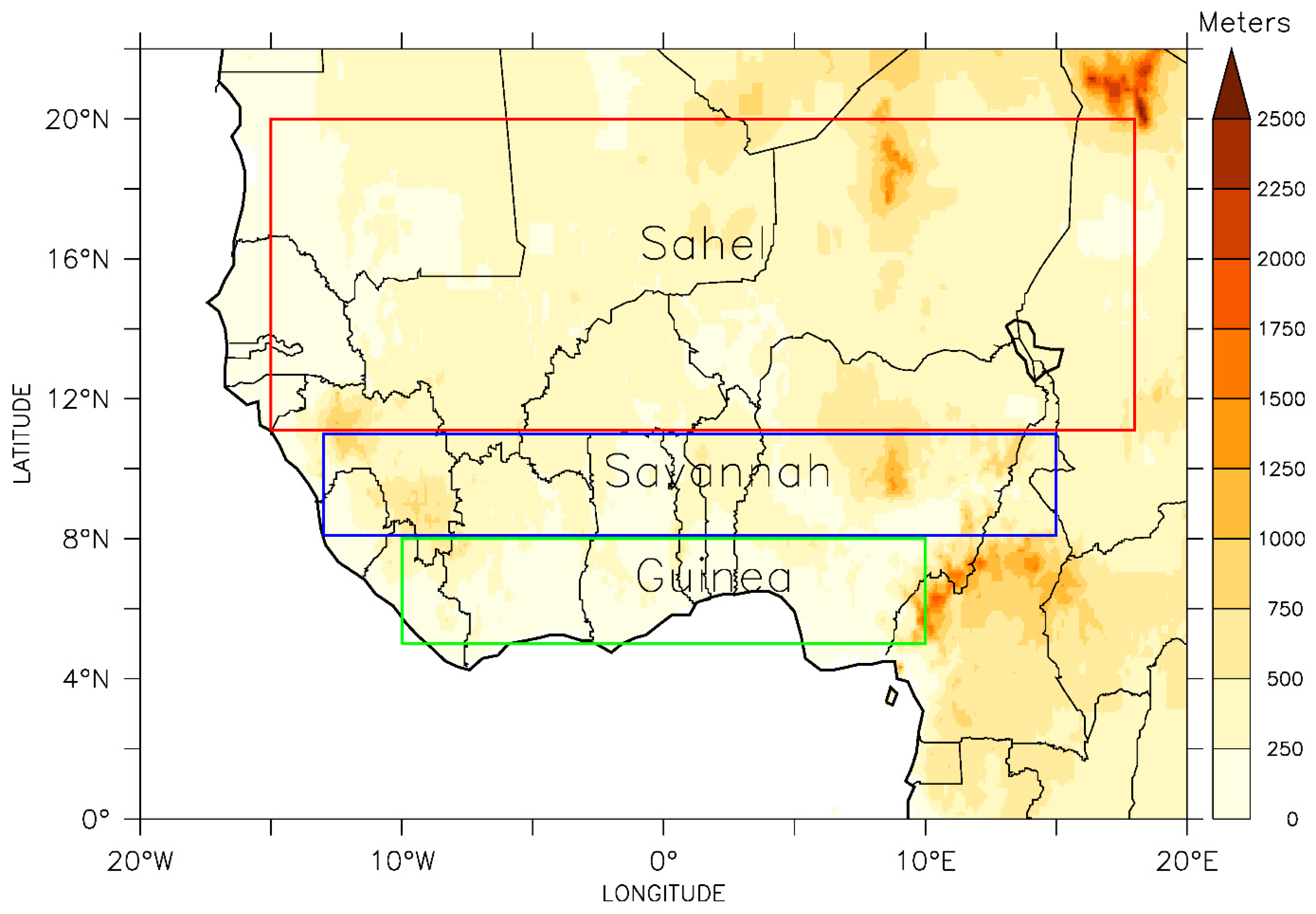
2.1. Description of Study Area
2.2. Datasets—Observation, Reanalysis, and Simulation Datasets
2.3. Methodology and Analysis Procedures

| Attributes | Descriptive Statistics | Inference |
|---|---|---|
| Reliability | Climatology | To determine the monthly, seasonal, or annual cycle of a variable [64]. |
| Bias (B) | A measure of over- (positive bias) or under-estimations (negative bias) of variables. Generally, bias gives marginal distributions of variables [11]. | |
| Mean bias error (MBE) | A measure to estimate the average bias in the model. It is the average forecast or simulation error representing the systematic error of a model to under- or over-forecast [11]. | |
| Scatter diagrams | Provides information on bias, outliers, error magnitude, linear association, peculiar behaviors in extremes, misses, and false alarms. Perfect simulation points in comparison to observation should be on the 45° diagonal line [17,65]. | |
| Association | ** Correlation coefficient (r) | A statistical measure of the strength of a linear relationship between the paired variables, i.e., simulations and observation/reanalysis datasets. By design, it is constrained as −1 ≤ r ≤ 1. Positive values denote direct linear association; negative values denote inverse linear association; a value of 0 denotes no linear association; while the closer the value is to 1 or −1, the stronger the linear association. Perfect relationship is denoted by 1. It is not sensitive to the bias but sensitive to outliers that may be present in the simulations [10,15,16]. |
| Coefficient of determination (CoD) | CoD is a measure of potential skill, i.e., the level of skill attainable when the biases are eliminated. It is also a measure of the fit of regression between forecast and observation. It is a non-negative parameter with a maximum value of 1. For a perfect regression, CoD = 1. CoD tends zero for a non-useful forecast [10,16]. | |
| Skill | Ranked probability skill score (RPSS) | Measures the forecast accuracy with respect to a reference forecast (e.g., observed climatology). Positive values (maximum of 1) have skill while negative values (up to negative infinity) have no skill [10,14,17,18,19]. |
| Accuracy | Mean absolute error (MAE) | A measure of how big of an error we can expect from the forecast on average, without considering their directions. MAE measures the accuracy of a continuous variable. Though, just like the root mean square error (RMSE), it also measures the average magnitude of the errors in a set of forecasts; however, while RMSE utilizes a quadratic scoring rule, MAE is a linear score—which means that all the individual differences are weighted equally in the average. MAE ranges from zero to infinity. Lower values are better [10,66,67]. |
| Root mean square error (RMSE) | It measures the magnitudes of the error, weighted on the squares of the errors. Though, it does not indicate the direction of the error; however, it is good in penalizing large errors. It is sensitive to large values (e.g., in precipitation) and outliers. This is very useful when large errors are undesirable. Ranges from zero to infinity. Lower values are better [10,68,69]. | |
| Synchronization (Syn) | Synchronization focuses on the predictive capabilities of a model. It shows how much a simulated value agrees with an observed value in the signs of their anomalies without taking magnitudes into consideration. Therefore, the evaluated synchronization, in a probabilistic sense, is similar to accuracy. The best synchronization is 100% [10,13,70,71]. | |
| Precision | Standard deviation (Std) | Std helps to determine the spread of simulations and/or observations from their respective means, i.e., how far from the mean a group of numbers is. It has the same unit as the mean [10,21,72,73]. |
| Coefficient of variation (CoV) | It is used for comparing the degree of variation from one data series to another (in this case between forecast or simulation and observation where the means are significantly different from one another). A lower CoV implies a low degree of variation while a higher CoV implies a higher variation. Therefore, the higher the CoV, the greater the level of spreading around the mean [10,21]. | |
| Normalized standard deviation (NSD) | This makes it possible to access the statistics of different fields (observations and simulations) on the same scale. Here, Taylor diagrams are used to depict the normalized standard deviation in line with correlation coefficients. The diagrams are able to measure how well observations and simulations match each other in terms of 1. similarity as measured by correlation coefficients, and 2. deviation factors as measured by normalized standard deviations. Taylor diagrams are able to provide a summarizing evaluation of model performance in simulating atmospheric parameters [10,21]. |
3. Results
3.1. Seasonality (and Reliability)
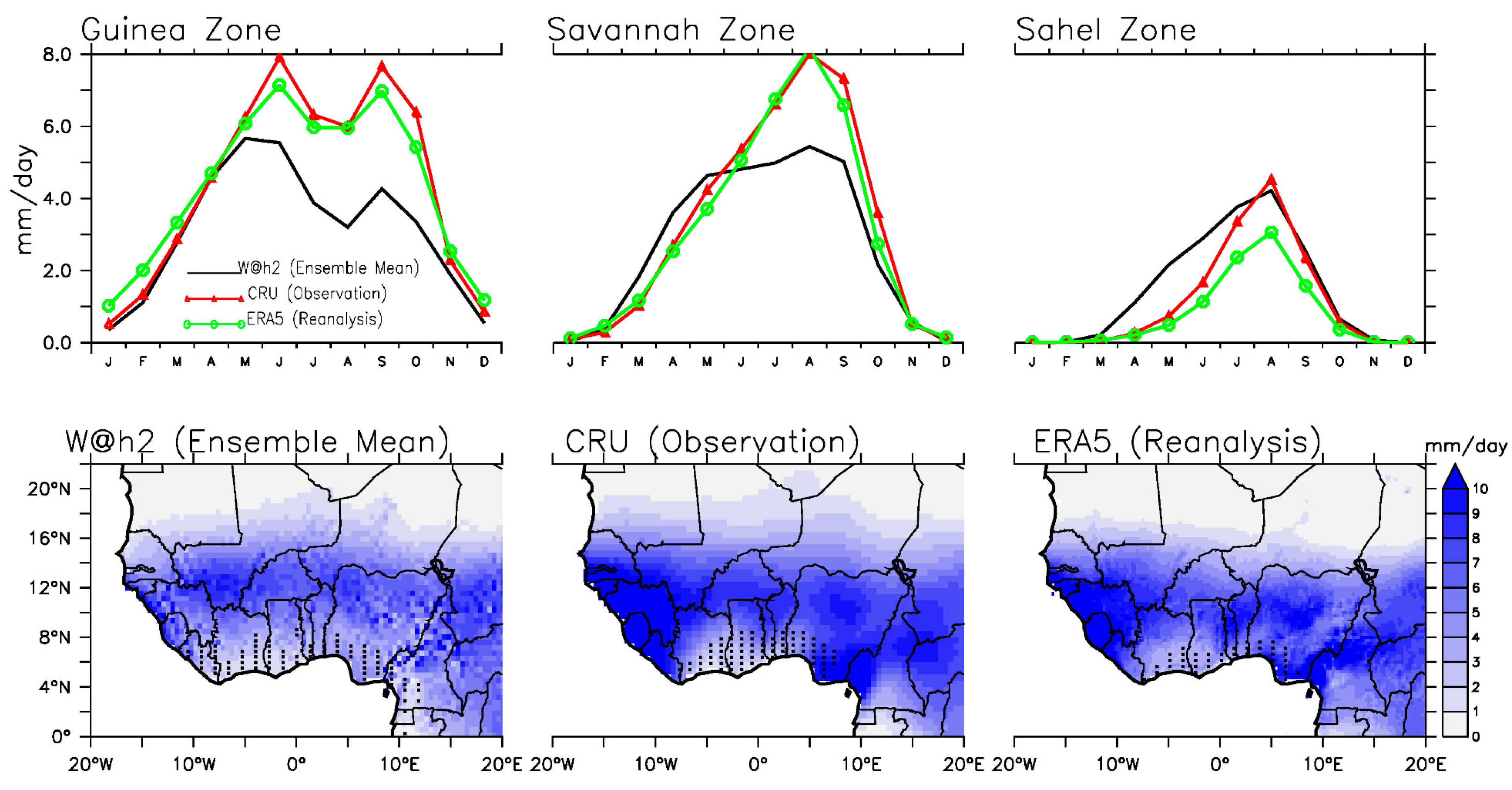
3.1.1. Precipitation
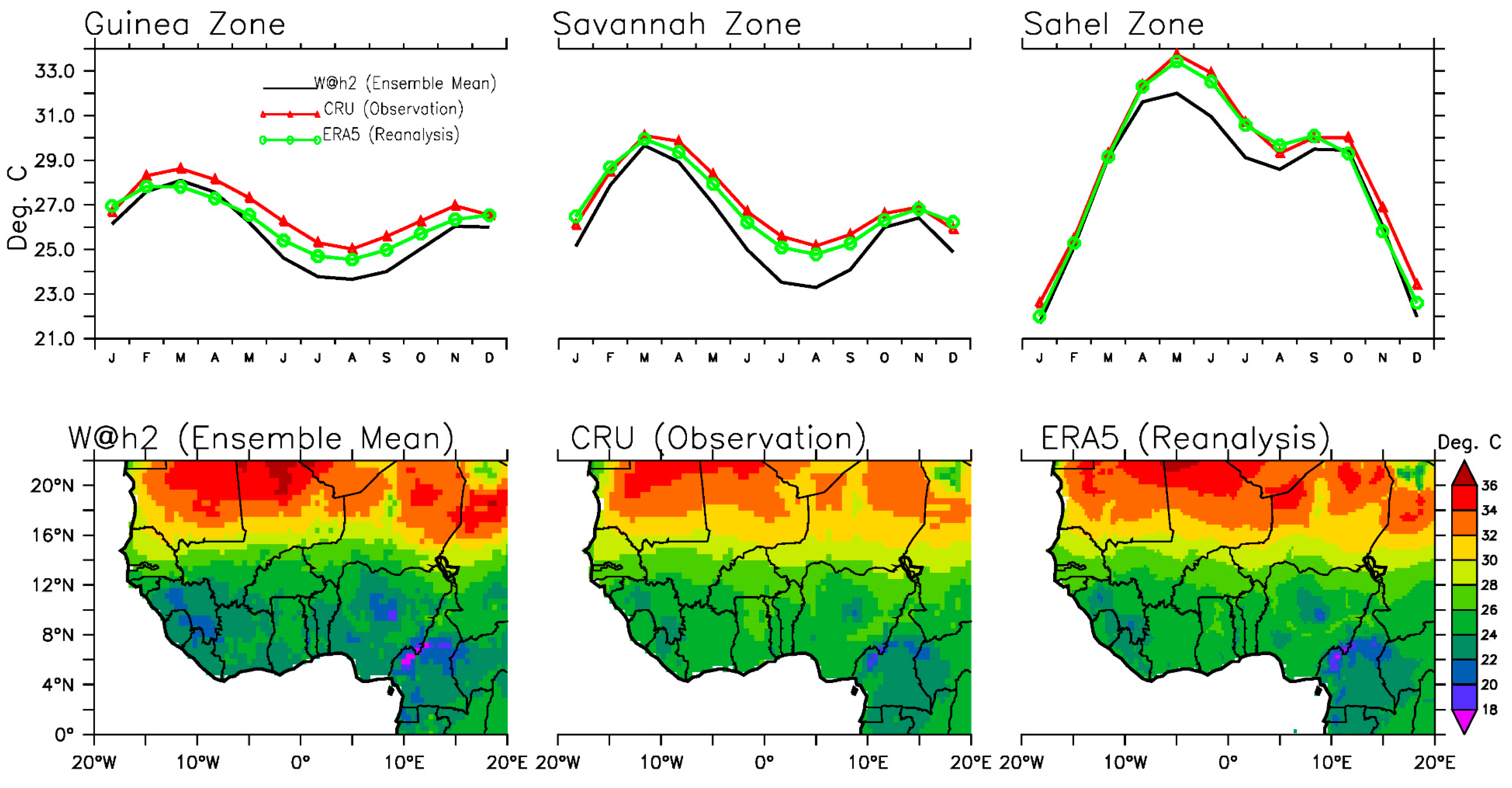
3.1.2. Temperature
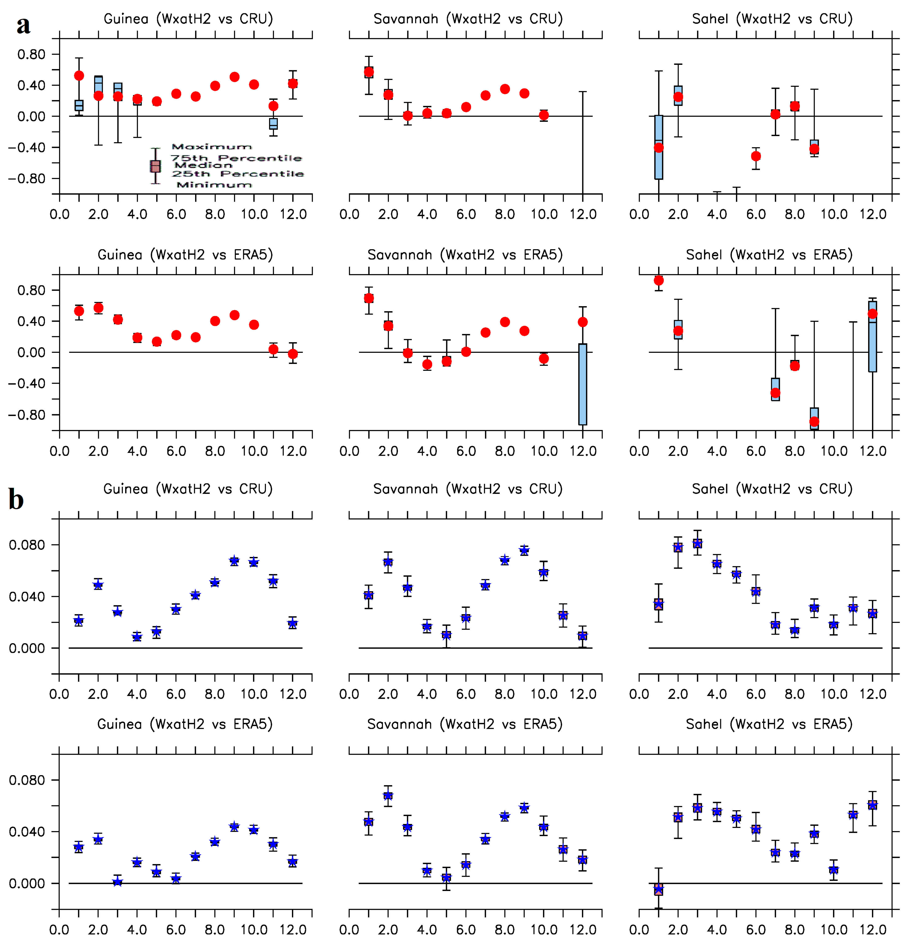
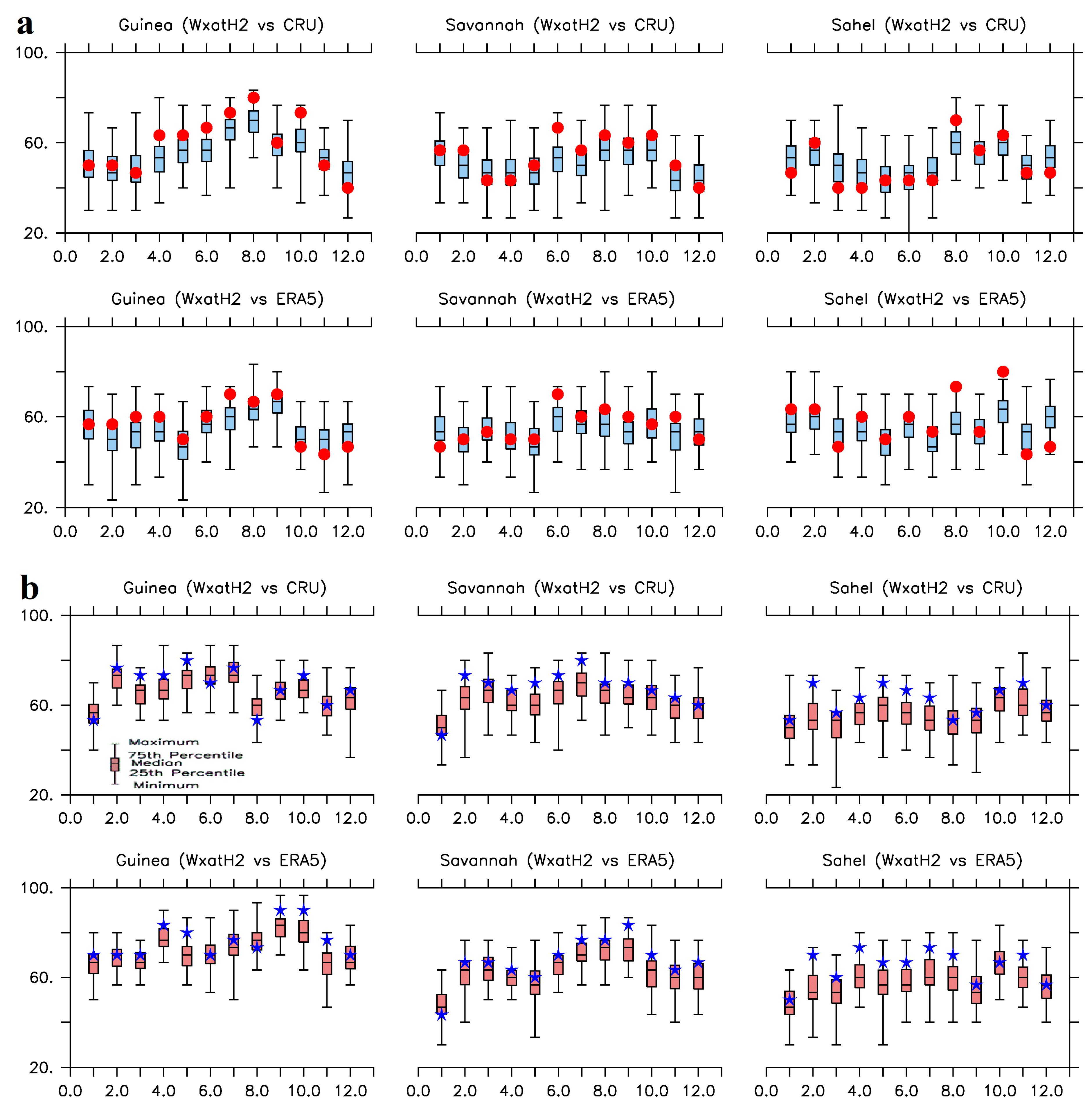
3.2. Association
3.3. Skill
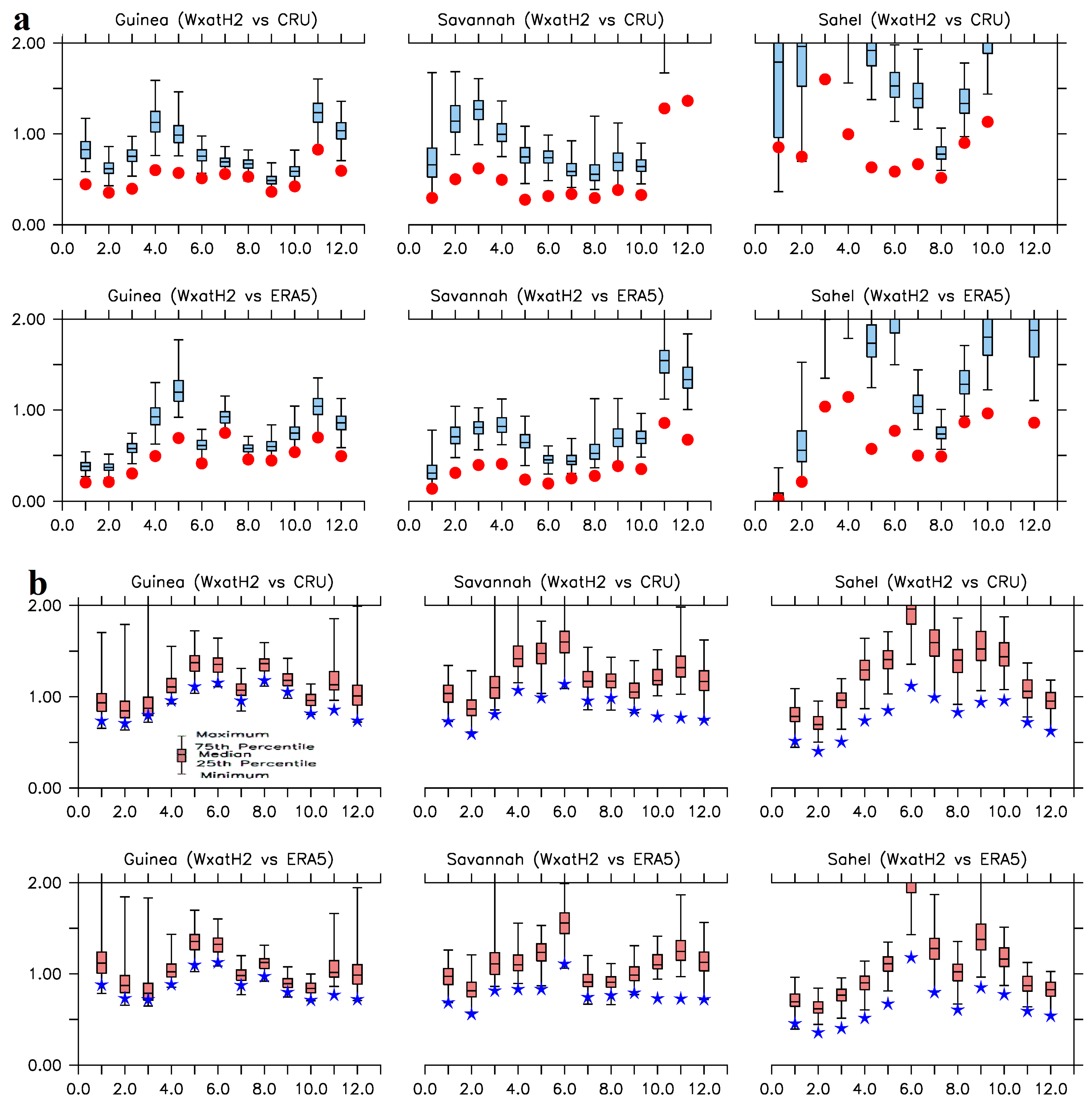
3.4. Accuracy
3.5. Precision
4. Discussion
Supplementary Materials
Author Contributions
Funding
Institutional Review Board Statement
Informed Consent Statement
Data Availability Statement
Acknowledgments
Conflicts of Interest
References
- Mariotti, L.; Coppola, E.; Sylla, M.B.; Giorgi, F.; Piani, C. Regional climate model simulation of projected 21st century climate change over an all-Africa domain: Comparison analysis of nested and driving model results. J. Geophys. Res. 2011, 116, D15111. [Google Scholar] [CrossRef]
- Nikulin, G.; Jones, C.; Giorgi, F.; Asrar, G.; Büchner, M.; Cerezo-Mota, R.; Christensen, O.B.; Déqué, M.; Fernandez, J.; Hänsler, A.; et al. Precipitation climatology in an ensemble of CORDEX-Africa regional climate simulations. J. Clim. 2012, 25, 6057–6078. [Google Scholar] [CrossRef]
- Diallo, I.; Sylla, M.B.; Camara, M.; Gaye, A.T. Inter-annual variability of rainfall over the Sahel based on multiple regional climate models simulations. Theor. Appl. Climatol. 2013, 113, 351–362. [Google Scholar] [CrossRef]
- Klein, C.; Heinzeller, D.; Bliefernicht, J.; Kunstman, H. Variability of West African monsoon patterns generated by a WRF Multiphysics ensemble. Clim. Dyn. 2015, 45, 2733–2755. [Google Scholar] [CrossRef]
- Sylla, M.B.; Giorgi, F.; Pal, J.S.; Gibba, P.; Kebe, I.; Nikiema, M. Projected changes in the annual cycle of high intensity precipitation events over West Africa for the late 21st century. J. Clim. 2015, 28, 6475–6488. [Google Scholar] [CrossRef]
- Tall, A.; Mason, S.J.; Van Aalst, M.; Suarez, P.; Ait-Chellouche, Y.; Diallo, A.A.; Braman, L. Using seasonal climate forecasts to guide disaster management: The Red Cross experience during the 2008 West Africa floods. Int. J. Geophys. 2012, 2012, 986016. [Google Scholar] [CrossRef]
- Niang, I.; Ruppel, O.; Abdrabo, M.; Essel, A.; Lennard, C.; Padgham, J.; Urquhart, P. Africa. In Climate Change 2014: Impacts, Adaptation and Vulnerability—Contributions of the Working Group II to the Fifth Assessment Report of the Intergovernmental Panel on Climate Change; Cambridge University Press: Cambridge, UK; New York, NY, USA, 2014; pp. 1199–1265. [Google Scholar]
- Nkiaka, E.; Taylor, A.; Dougill, A.; Antwi-Agyei, P.; Fournier, N.; Bosire, E.; Konte, O.; Lawal, K.A.; Mutai, B.; Mwangi, E.; et al. Identifying user needs for weather and climate services to enhance resilience to climate shocks in sub-Saharan Africa. Environ. Res. Lett. 2019, 14, 123003. [Google Scholar] [CrossRef]
- Lundstad, E.; Brugnara, Y.; Pappert, D.; Kopp, J.; Samakinwa, E.; Hürzeler, A.; Andersson, A.; Chimani, B.; Cornes, R.; Demarée, G.; et al. The global historical climate database HCLIM. Sci. Data 2023, 10, 44. [Google Scholar] [CrossRef]
- Storch, H.V.; Zwiers, F.W. Statistical Analysis in Climate Research; Cambridge University Press: London, UK, 2003. [Google Scholar]
- Walther, B.A.; Moore, J.L. The concepts of bias, precision and accuracy, and their use in testing the performance of species richness estimators, with a literature review of estimator performance. Ecography 2005, 28, 815–829. [Google Scholar] [CrossRef]
- Ebert, E.; Wilson, L.; Weigel, A.; Mittermaier, M.; Nurmi, P.; Gill, P.; Gober, M.; Joslyn, S.; Brown, B.; Fowlerh, T.; et al. Progress and challenges in forecast verification. Meteorol. Appl. 2013, 20, 130–139. [Google Scholar] [CrossRef]
- Wilson, L.J.; Giles, A. A new index for the verification of accuracy and timeliness of weather warnings. Meteorol. Appl. 2013, 20, 206–216. [Google Scholar] [CrossRef]
- Mason, S.J. On using “climatology” as a reference strategy in the brier and ranked probability skill scores. Mon. Weather Rev. 2004, 132, 1891–1895. [Google Scholar]
- Murphy, A.H. Skill score on the mean square error and their relationship to the correlation coefficient. Mon. Weather Rev. 1988, 116, 2417–2424. [Google Scholar]
- Murphy, A.H. The coefficients of correlation and determination as measures of performance in forecast verification. Weather Forecast. 1995, 10, 681–688. [Google Scholar]
- Wilks, D.S. Statistical Methods in Atmospheric Sciences: An Introduction, 2nd ed.; Academic Press: San Diego, CA, USA, 1995. [Google Scholar]
- Weigel, A.P.; Liniger, M.A.; Appenzeller, C. The discrete brier and ranked probability skill scores. Mon. Weather Rev. 2006, 135, 118–124. [Google Scholar]
- Kim, G.; Ahn, J.-B.; Kryjov, V.N.; Sohn, S.-J.; Yun, W.-T.; Graham, R.; Kolli, R.K.; Kumar, A.; Ceron, J.-P. Global and regional skill of the seasonal predictions by WMO Lead Centre for Long-Range Forecast Multi-Model Ensemble. Int. J. Climatol. 2016, 36, 1657–1675. [Google Scholar] [CrossRef]
- Debanne, S.M. The planning of clinical studies: Bias and precision. Gastrointest. Endosc. 2000, 52, 821–822. [Google Scholar]
- West, M.J. Stereological methods for estimating the total number of neurons and synapses: Issues of precision and bias. Trends Neurosci. 1999, 22, 51–61. [Google Scholar] [PubMed]
- Xue, Y.; De Sales, F.; Lau, K.M.W.; Bonne, A.; Feng, J.; Dirmeyer, P.; Guo, Z.; Kim, K.M.; Kitoh, A.; Kumar, V.; et al. Intercomparison of West African Monsoon and its variability in the West African Monsoon Modelling Evaluation Project (WAMME) first model inter-comparison experiment. Clim. Dyn. 2010, 35, 3–27. [Google Scholar] [CrossRef]
- Verdin, A.; Funk, C.; Peterson, P.; Landsfeld, M.; Tuholske, C.; Grace, K. Development and validation of the CHIRTS-daily quasi-global high-resolution daily temperature data set. Sci. Data 2020, 7, 303. [Google Scholar] [CrossRef]
- Zaroug, M.A.H.; Sylla, M.B.; Giorgi, F.; Eltahir, E.A.B.; Aggarwal, P.K. A sensitivity study on the role of the Swamps of Southern Sudan in the summer climate of North Africa using a regional climate model. Theor. Appl. Climatol. 2013, 113, 63–81. [Google Scholar] [CrossRef]
- Diallo, I.; Bain, C.L.; Gaye, A.T.; Moufouma-Okia, W.; Niang, C.; Dieng, M.D.B.; Graham, R. Simulation of the West African monsoon onset using the HadGEM3-RA regional climate model. Clim. Dyn. 2014, 45, 575–594. [Google Scholar] [CrossRef]
- Massey, N.; Jones, R.; Otto, F.E.L.; Aina, T.; Wilson, S.; Murphy, J.M.; Hassell, D.; Yamazaki, Y.H.; Allen, M.R. weather@home—Development and validation of a very large ensemble modelling system for probabilistic event attribution. Q. J. Roy. Meteor. Soc. 2015, 141, 1528–1545. [Google Scholar] [CrossRef]
- Guillod, B.P.; Jones, R.G.; Bowery, A.; Haustein, K.; Massey, N.R.; Mitchell, D.M.; Otto, F.E.L.; Sparrow, S.N.; Uhe, P.; Wallom, D.C.H.; et al. weather@home 2: Validation of an improved global–regional climate modelling system. Geosci. Model Dev. 2017, 10, 1849–1872. [Google Scholar] [CrossRef]
- Wood, R.R.; Lehner, F.; Pendergrass, A.G.; Schlunegger, S. Changes in precipitation variability across time scales in multiple global climate model large ensembles. Environ. Res. Lett. 2021, 16, 084022. [Google Scholar] [CrossRef]
- Bellprat, O.; Doblas-Reyes, F. Attribution of extreme weather and climate events overestimated by unreliable climate simulations. Geophys. Res. Lett. 2016, 43, 2158–2164. [Google Scholar] [CrossRef]
- Lott, F.C.; Stott, P.A. Evaluating Simulated Fraction of Attributable Risk Using Climate Observations. J. Clim. 2016, 29, 4565–4575. [Google Scholar] [CrossRef]
- Bellprat, O.; Guemas, V.; Doblas-Reyes, F.; Donat, M.G. Towards reliable extreme weather and climate event attribution. Nat. Commun. 2019, 10, 1732. [Google Scholar] [CrossRef]
- Nicholson, S.E.; Palao, I.M. A Re-evaluation of rainfall variability in the Sahel. Part I. Characteristics of rainfall fluctuations. Int. J. Climatol. 1993, 13, 371–389. [Google Scholar]
- Nicholson, S.E. Sahel, West Africa. Encycl. Environ. Biol. 1995, 3, 261–275. [Google Scholar]
- Omotosho, J.B.; Abiodun, B.J. A numerical study of moisture build-up and rainfall over West Africa. Meteorol. Appl. 2007, 14, 209–225. [Google Scholar] [CrossRef]
- Omotosho, J.B. Pre-rainy season moisture build-up and storm precipitation delivery in the West Africa Sahel. Int. J. Climatol. 2007, 28, 937–946. [Google Scholar] [CrossRef]
- Nicholson, S.E. An overview of African rainfall fluctuations of the last decade. J. Clim. 1993, 6, 1463–1466. [Google Scholar]
- Latif, M.; Grotzner, A. On the equatorial Atlantic oscillation and its response to ENSO. Clim. Dyn. 2000, 16, 213–218. [Google Scholar]
- Camberlin, P.; Janicot, S.; Poccard, I. Seasonality and atmospheric dynamics of the teleconnection between African rainfall and tropical sea-surface temperature: Atlantic vs. ENSO. Int. J. Climatol. 2001, 21, 973–1005. [Google Scholar] [CrossRef]
- Newman, M.; Sardeshmukh, P.D.; Winkler, C.R.; Whitaker, J.S. A study of sub-seasonal predictability. Mon. Weather Rev. 2003, 131, 1715–1732. [Google Scholar] [CrossRef]
- Odekunle, T.O.; Eludoyin, A.O. Sea surface temperature patterns in the Gulf of Guinea: Their implications for the spatio-temporal variability of precipitation in West Africa. Int. J. Climatol. 2008, 28, 1507–1517. [Google Scholar] [CrossRef]
- Diedhiou, A.; Janicot, S.; Viltard, A.; de Felice, P. Evidence of two regimes of easterly waves over West Africa and the tropical Atlantic. Geophys. Res. Lett. 1998, 25, 2805–2808. [Google Scholar]
- Grist, J.P.; Nicholson, S.E. Easterly waves over Africa. Part II: Observed and modeled contrasts between wet and dry years. Mon. Weather Rev. 2001, 130, 212–225. [Google Scholar] [CrossRef]
- Afiesimama, E.A. Annual cycle of the mid-tropospheric easterly jet over West Africa. Theor. Appl. Climatol. 2007, 90, 103–111. [Google Scholar] [CrossRef]
- Parker, D.J.; Thorncroft, C.D.; Burton, R.; Diongue-Niang, A. Analysis of the African easterly jet, using aircraft observations from the JET 2000 experiment. Q. J. R. Meteorol. Soc. 2005, 131, 1461–1482. [Google Scholar] [CrossRef]
- Lavaysse, C.; Diedhiou, A.; Laurent, H.; Lebel, T. African easterly waves and convective activity in wet and dry sequences of the West African monsoon. Clim. Dyn. 2006, 27, 319–332. [Google Scholar] [CrossRef]
- Lavaysse, C.; Flamant, C.; Janicot, S.; Parker, D.J.; Lafore, J.-P.; Sultan, B. Seasonal evolution of the West African heat low: A climatological perspective. Clim. Dyn. 2009, 33, 313–330. [Google Scholar] [CrossRef]
- Lavaysse, C.; Flamant, C.; Janicot, S.; Knippertz, P. Links between African easterly waves, midlatitude circulation and intraseasonal pulsations of the West African heat low. Q. J. R. Meteorol. Soc. 2010, 136, 141–158. [Google Scholar] [CrossRef]
- Nicholson, S.E.; Grist, J.P. The seasonal evolution of the atmospheric circulation over West Africa and equatorial Africa. J. Clim. 2003, 16, 1013–1030. [Google Scholar]
- Redelsperger, J.-L.; Thorncroft, C.D.; Diedhiou, A.; Lebel, T.; Paker, D.J.; Polcher, J. African Monsoon Multidisciplinary Analysis: An international research project and field Campaign. Bull. Am. Meteorol. Soc. 2006, 87, 1739–1746. [Google Scholar]
- CRU TS Version 4.03. Available online: https://crudata.uea.ac.uk/cru/data/hrg/cru_ts_4.03/ (accessed on 31 January 2025).
- New, M.; Hulme, M.; Jones, P.D. Representing twentieth century space-time climate variability. Part 2: Development of 1901-96 monthly grids of terrestrial surface climate. J. Clim. 2000, 13, 2217–2238. [Google Scholar] [CrossRef]
- Harris, I.; Osborn, T.J.; Jones, P.; Lister, D. Version 4 of the CRU TS monthly high-resolution gridded multivariate climate dataset. Sci. Data 2020, 7, 109. [Google Scholar] [CrossRef]
- European Centre for Medium-Range Weather Forecasts (ECMWF—ERA Version 5 (ERA5). Available online: https://www.ecmwf.int/en/forecasts/datasets/reanalysis-datasets/era5 (accessed on 31 January 2025).
- Hersbach, H.; de Rosnay, P.; Bell, B.; Schepers, D.; Simmons, A.; Soci, C.; Abdalla, S.; Balmaseda, M.A.; Balsamo, G.; Bechtold, P.; et al. Operational Global Reanalysis: Progress, Future Directions and Synergies with NWP; ERA Report Series, No. 27; ECMWF: London, UK, 2018. [Google Scholar]
- Steinkopf, J.; Engelbrecht, F. Verification of ERA5 and ERA-Interim precipitation over Africa at intra-annual and interannual timescales. Atmos. Res. 2022, 280, 106427. [Google Scholar] [CrossRef]
- CPDN. Available online: https://www.climateprediction.net (accessed on 31 January 2025).
- Jones, R.G.; Noguer, M.; Hassell, D.C.; Hudson, D.; Willson, S.S.; Genkins, G.J.; Mitchell, J.F.B. Generating High Resolution Climate Change Scenarios Using PRECIS; Technical report; Met Office Hadley Centre: Exeter, UK, 2004; 40p. [Google Scholar]
- Essery, R.; Clark, D.B. Developments in the MOSES 2 land surface model for PILPS 2e. Glob. Planet. Change 2003, 38, 161–164. [Google Scholar] [CrossRef]
- Donlon, C.J.; Martin, M.; Stark, J.; Roberts-Jones, J.; Fiedler, E.; Wimmer, W. The Operational Sea Surface Temperature and Sea Ice Analysis (OSTIA) system. Remote Sens. Environ. 2012, 116, 140–158. [Google Scholar] [CrossRef]
- Anderson, D.P. Boinc: A system for public-resource computing and storage. In Proceedings of the Fifth IEEE/ACM International Workshop on Grid Computing, Pittsburgh, PA, USA, 8 November 2004; IEEE: Piscataway, NJ, USA, 2004; pp. 4–10. [Google Scholar]
- Black, M.T.; Karoly, D.J.; Rosier, S.M.; Dean, S.M.; King, A.D.; Massey, N.R.; Sparrow, S.N.; Bowery, A.; Wallom, D.; Jones, R.G.; et al. The weather@home regional climate modelling project for Australia and New Zealand. Geosci. Model Dev. 2016, 9, 3161–3176. [Google Scholar] [CrossRef]
- Lawal, K.A.; Abiodun, B.J.; Stone, D.A.; Olaniyan, E.; Wehner, M.F. Capability of CAM5.1 in simulating maximum air temperature anomaly patterns over West Africa during boreal spring. Model. Earth Syst. Environ. 2019, 5, 1815–1838. [Google Scholar] [CrossRef]
- Mason, S.J. Understanding forecast verification statistics. Meteorol. Appl. 2008, 15, 31–40. [Google Scholar] [CrossRef]
- Hidore, J.J.; Oliver, J.E.; Snow, M.; Snow, R. Climatology: An Atmospheric Science, 3rd ed.; Pearson: San Francisco, CA, USA, 2009; ISBN-10: 0321602056/ISBN-13: 978-0321602053. [Google Scholar]
- Jolliffe, I.T.; Stephenson, D.B. Forecast Verification: A Practitioner’s Guide in Atmospheric Science, 1st ed.; John Wiley & Sons, Ltd.: Berlin/Heidelberg, Germany, 2012; Print ISBN 9780470660713/Online ISBN 9781119960003. [Google Scholar] [CrossRef]
- Pledger, S. Unified maximum likelihood estimates for cloud capture-recapture models using mixtures. Biometrics 2000, 56, 434–442. [Google Scholar] [CrossRef]
- Pledger, S.; Schwarz, C.J. Modelling heterogeneity of survival in band-recovery data using mixtures. J. Appl. Stat. 2002, 29, 315–327. [Google Scholar] [CrossRef]
- Rosenberg, D.K.; Everton, W.S.; Anthony, R.G. Estimation of animal abundance when capture probabilities are low and heterogenous. J. Wildl. Manag. 1995, 59, 252–261. [Google Scholar] [CrossRef]
- Zelmer, D.A.; Esch, G.W. Robust estimation of parasite component community richness. J. Parasitol. 1999, 85, 592–594. [Google Scholar]
- Misra, J. Phase synchronization. Inf. Process. Lett. 1991, 38, 101–105. [Google Scholar] [CrossRef]
- Lawal, K.A. Understanding the Variability and Predictability of Seasonal Climates over West and Southern Africa Using Climate Models. Ph.D. Thesis, Faculty of Sciences, University of Cape Town, Cape Town, South Africa, 2015. Available online: https://open.uct.ac.za/handle/11427/16556?show=full (accessed on 31 January 2025).
- Brose, U.; Martinez, N.D.; Williams, R.J. Estimating species richness: Sensitivity to sample coverage and insensitivity to spatial patterns. Ecology 2003, 84, 2364–2377. [Google Scholar] [CrossRef]
- Melo, A.S.; Pereira, R.A.S.; Santos, A.J.; Shepherd, G.J.; Machado, G.; Medeiros, H.F.; Sawaya, R.J. Comparing species richness among assemblages using sample units: Why not use extrapolation methods to standardize different sample sizes? Oikos 2003, 101, 398–410. [Google Scholar] [CrossRef]
- Cook, K.H.; Vizy, E.K. Detection and Analysis of an Amplified Warming of the Sahara Desert. J. Clim. 2015, 28, 6560–6580. [Google Scholar] [CrossRef]
- Nicholson, S.E. Climatic and environmental change in Africa during the last two centuries. Clim. Res. 2001, 17, 123–144. [Google Scholar] [CrossRef]
- Nicholson, S.E. On the factors modulating the intensity of the tropical rain belt over West Africa. Int. J. Climatol. 2009, 29, 673–689. [Google Scholar] [CrossRef]
- Olaniyan, E.; Adefisan, A.E.; Oni, F.; Afiesimama, E.; Balogun, A.; Lawal, K.A. Evaluation of the ECMWF Sub-seasonal to Seasonal Precipitation Forecasts During the Peak of West Africa Monsoon in Nigeria. Front. Environ. Sci. 2017, 6, 1–15. [Google Scholar] [CrossRef]
- Ehrendorfer, M. Predicting the uncertainty of numerical weather forecasts: A review. Meteor Z 1997, 6, 147–183. [Google Scholar]
- Hamill, T.M.; Colucci, S.J. Verification of Eta–RSM short-range ensemble forecasts. Mon. Weather Rev. 1997, 125, 1312–1327. [Google Scholar]
- Palmer, T.N. Predicting uncertainty in forecasts of weather and climate. Rep. Prog. Phys. 2000, 63, 71–116. [Google Scholar]
- Stensrud, D.J.; Bao, J.-W.; Warner, T.T. Using initial condition and model physics perturbations in short-range ensemble simulations of mesoscale convective systems. Mon. Weather Rev. 2000, 128, 2077–2107. [Google Scholar]
- Stensrud, D.J.; Yussouf, N. Short-range ensemble predictions of 2-m temperature and dew-point temperature over New England. Mon. Weather Rev. 2003, 131, 2510–2524. [Google Scholar] [CrossRef]
- Jankov, I.; Gallus, W.A., Jr.; Segal, M.; Shaw, B.; Koch, S.E. The impact of different WRF model physical parameterizations and their interactions on warm season MCS rainfall. Weather Forecast. 2005, 20, 1048–1060. [Google Scholar] [CrossRef]
- Deser, C.; Lehner, F.; Rodgers, K.B.; Ault, T.; Delworth, T.L.; DiNezio, P.N.; Fiore, A.; Frankignoul, C.; Fyfe, J.C.; Horton, D.E.; et al. Insights from Earth system model initial-condition large ensembles and future prospects. Nat. Clim. Change 2020, 10, 277–286. [Google Scholar] [CrossRef]
- Risser, M.D.; Stone, D.A.; Paciorek, C.J.; Wehner, M.F.; Angélil, O. Quantifying the effect of interannual ocean variability on the attribution of extreme climate events to human influence. Clim. Dyn. 2017, 49, 3051–3073. [Google Scholar] [CrossRef]
- Tanimoune, L.I.; Smiatek, G.; Kunstmann, H.; Abiodun, B.J. Simulation of temperature extremes over West Africa with MPAS. J. Geophys. Res. Atmos. 2023, 128, e2023JD039055. [Google Scholar] [CrossRef]


Disclaimer/Publisher’s Note: The statements, opinions and data contained in all publications are solely those of the individual author(s) and contributor(s) and not of MDPI and/or the editor(s). MDPI and/or the editor(s) disclaim responsibility for any injury to people or property resulting from any ideas, methods, instructions or products referred to in the content. |
© 2025 by the authors. Licensee MDPI, Basel, Switzerland. This article is an open access article distributed under the terms and conditions of the Creative Commons Attribution (CC BY) license (https://creativecommons.org/licenses/by/4.0/).
Share and Cite
Lawal, K.A.; Akintomide, O.M.; Olaniyan, E.; Bowery, A.; Sparrow, S.N.; Wehner, M.F.; Stone, D.A. Performance Evaluation of Weather@home2 Simulations over West African Region. Atmosphere 2025, 16, 392. https://doi.org/10.3390/atmos16040392
Lawal KA, Akintomide OM, Olaniyan E, Bowery A, Sparrow SN, Wehner MF, Stone DA. Performance Evaluation of Weather@home2 Simulations over West African Region. Atmosphere. 2025; 16(4):392. https://doi.org/10.3390/atmos16040392
Chicago/Turabian StyleLawal, Kamoru Abiodun, Oluwatosin Motunrayo Akintomide, Eniola Olaniyan, Andrew Bowery, Sarah N. Sparrow, Michael F. Wehner, and Dáithí A. Stone. 2025. "Performance Evaluation of Weather@home2 Simulations over West African Region" Atmosphere 16, no. 4: 392. https://doi.org/10.3390/atmos16040392
APA StyleLawal, K. A., Akintomide, O. M., Olaniyan, E., Bowery, A., Sparrow, S. N., Wehner, M. F., & Stone, D. A. (2025). Performance Evaluation of Weather@home2 Simulations over West African Region. Atmosphere, 16(4), 392. https://doi.org/10.3390/atmos16040392