

Evaluating the Performance of Soil and Water Assessment Tool (SWAT) in a Snow-Dominated Climate (Case Study: Azna–Aligoudarz Basin, Iran)


Abstract
1. Introduction
2. Material and Methods
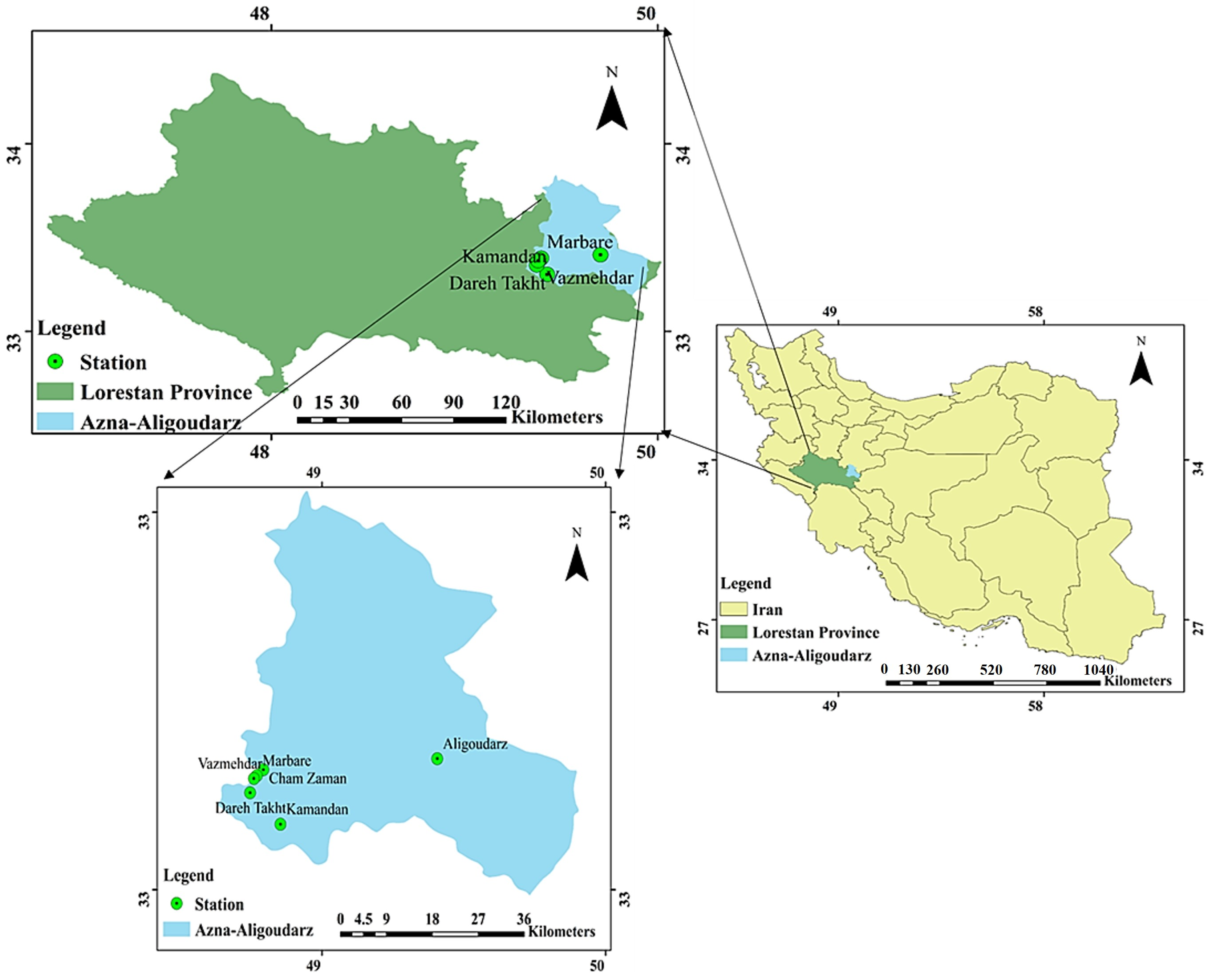
2.1. Study Area
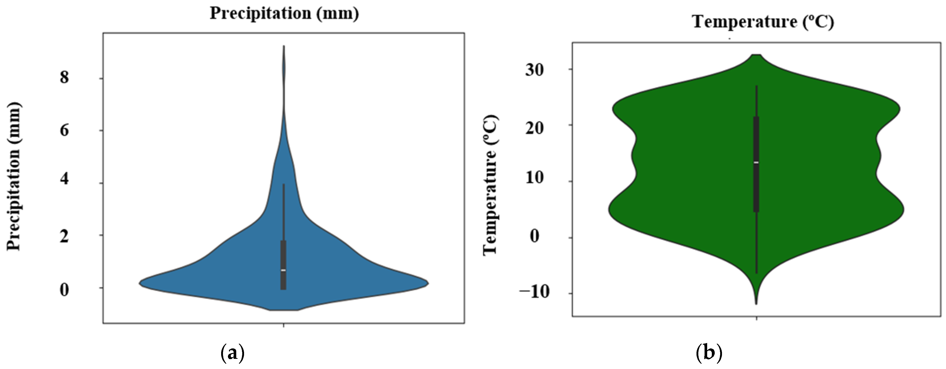
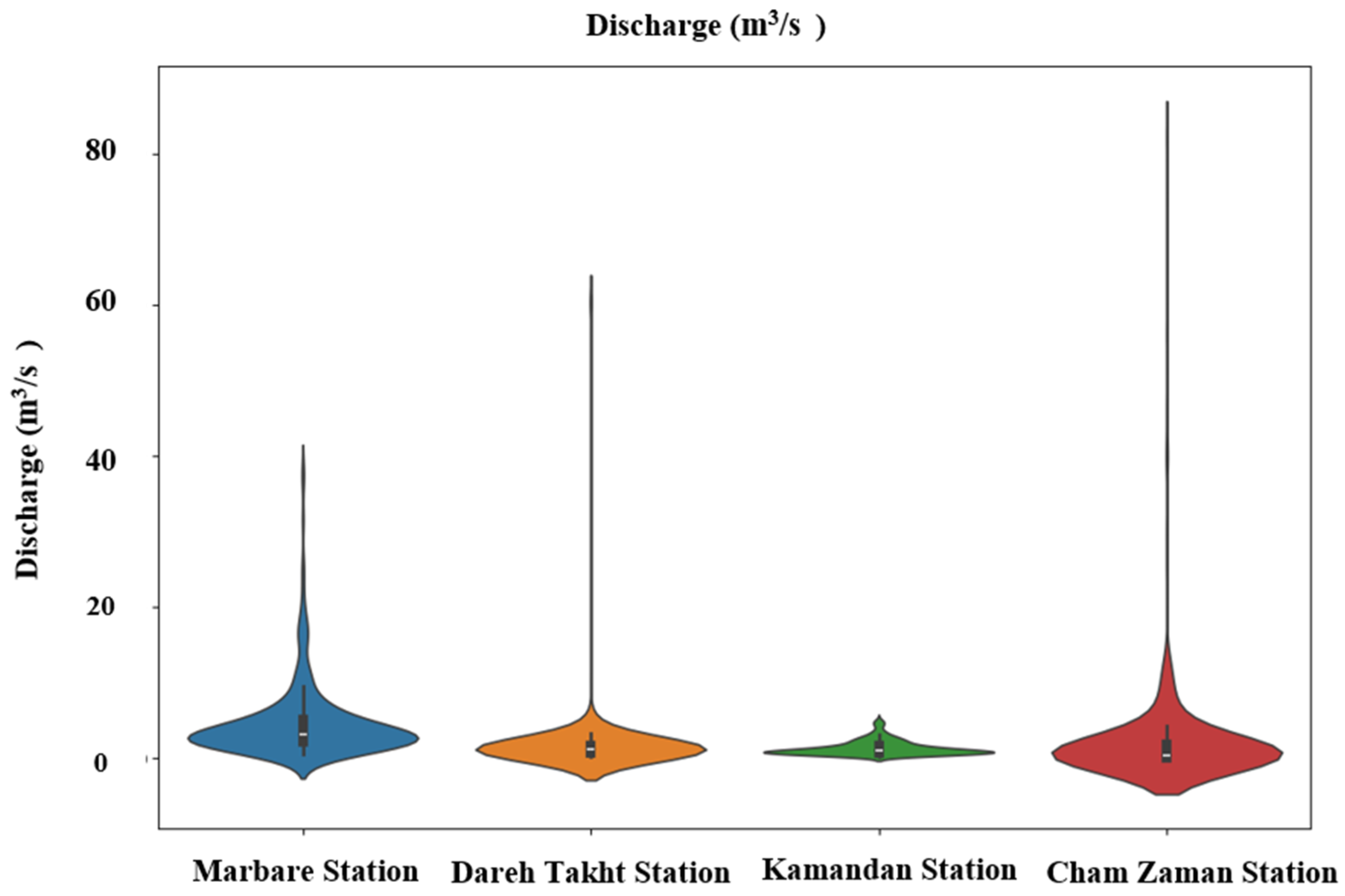
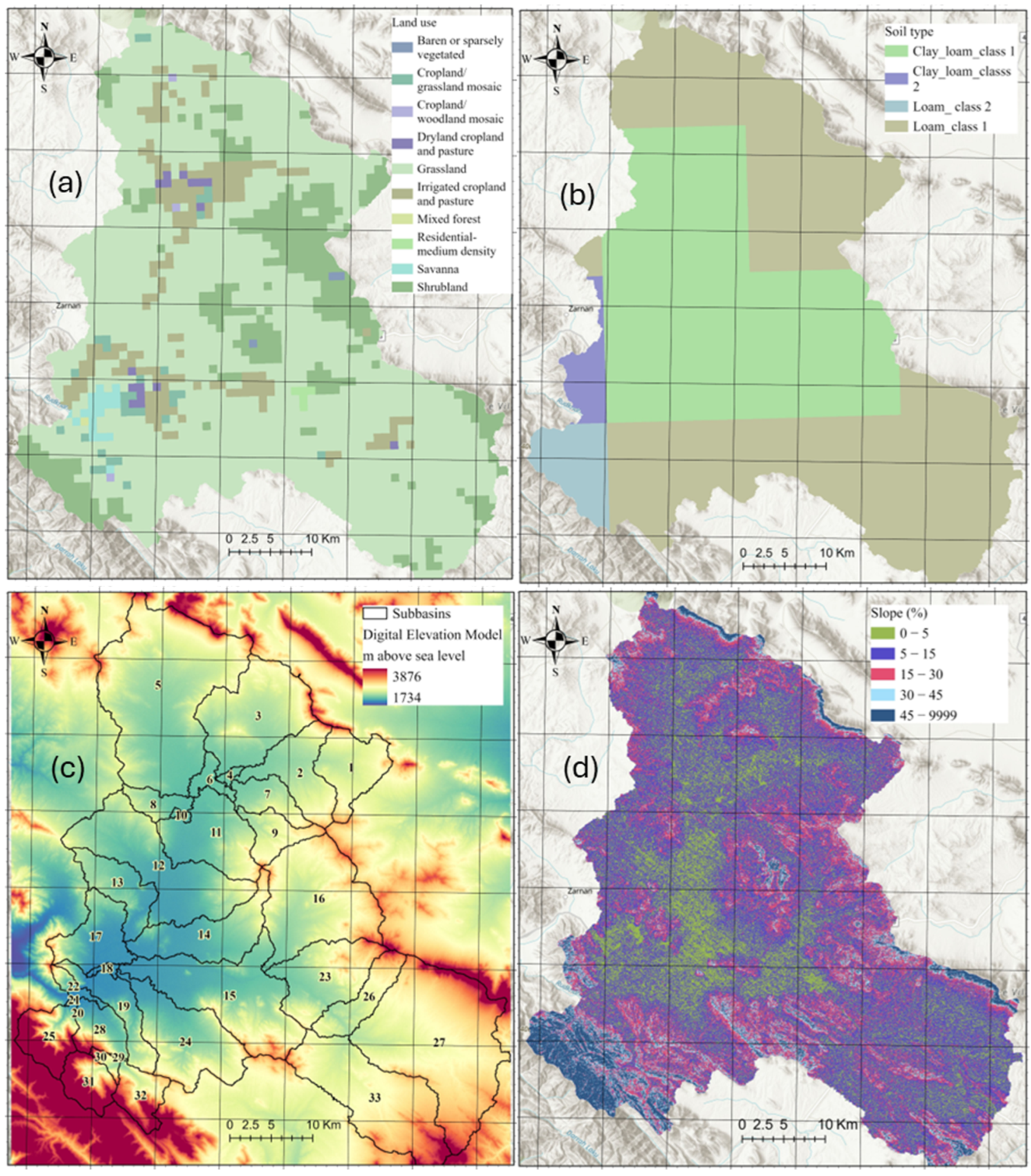
2.2. Data Description
2.3. Methodology
2.4. Theoretical Background of Snowmelt and Runoff Generation in SWAT
2.5. Curve Number Method
2.6. Snow Module in SWAT
2.7. Calibration, Validation, Sensitivity Analysis and Uncertainty Analysis Using SWAT-CUP
2.8. Application of SWAT to Simulate Study Area
2.9. Evaluation Criteria
3. Results
4. Discussion
5. Conclusions
Author Contributions
Funding
Institutional Review Board Statement
Informed Consent Statement
Data Availability Statement
Conflicts of Interest
References
- Vuille, M.; Carey, M.; Huggel, C.; Buytaert, W.; Rabatel, A.; Jacobsen, D.; Soruco, A.; Villacis, M.; Yarleque, C.; Timm, O.E.; et al. Rapid decline of snow and ice in the tropical Andes—Impacts, uncertainties and challenges ahead. Earth Sci. Rev. 2018, 176, 195–213. [Google Scholar]
- Dehban, H.; Zareian, M.J.; Gohari, A. Evaluating regional climate change during 2021–2080 for Iran and neighboring countries (a comparative analysis of projections and reanalysis data). Theor. Appl. Climatol. 2025, 156, 143. [Google Scholar]
- Akbari, S.; Gao, J.; Flores, J.P.; Smith, G. Evaluating Energy Performance of Windows in High-Rise Residential Buildings: A Thermal and Statistical Analysis. Preprints 2025. [Google Scholar] [CrossRef]
- Intergovernmental Panel on Climate Change (IPCC). High Mountain Areas. In The Ocean and Cryosphere in a Changing Climate: Special Report of the Intergovernmental Panel on Climate Change; Cambridge University Press: Cambridge, UK, 2022; pp. 131–202. [Google Scholar] [CrossRef]
- Baniya, R.; Regmi, R.K.; Talchabhadel, R.; Sharma, S.; Panthi, J.; Ghimire, G.R.; Bista, S.; Thapa, B.R.; Pradhan, A.M.S.; Tamrakar, J. Integrated modeling for assessing climate change impacts on water resources and hydropower potential in the Himalayas. Theor. Appl. Climatol. 2024, 155, 3993–4008. [Google Scholar] [CrossRef]
- Swalih, S.A.; Kahya, E. Performance of gridded precipitation products in the Black Sea region for hydrological studies. Theor. Appl. Climatol. 2022, 149, 465–485. [Google Scholar]
- Wang, J.; Kumar Shrestha, N.; Aghajani Delavar, M.; Worku Meshesha, T.; Bhanja, S.N. Modelling watershed and river basin processes in cold climate regions: A review. Water 2021, 13, 518. [Google Scholar] [CrossRef]
- Singh, V.P.; Woolhiser, D.A. Mathematical modeling of watershed hydrology. J. Hydrol. Eng. 2002, 7, 270–292. [Google Scholar]
- Devia, G.K.; Ganasri, B.P.; Dwarakish, G.S. A review on hydrological models. Aquat. Procedia 2015, 4, 1001–1007. [Google Scholar]
- Panchanthan, A.; Ahrari, A.H.; Ghag, K.; Mustafa, S.M.T.; Haghighi, A.T.; Kløve, B.; Oussalah, M. An overview of approaches for reducing uncertainties in hydrological forecasting: Progress and challenges. Earth-Sci. Rev. 2024, 258, 104956. [Google Scholar] [CrossRef]
- Arnold, J.G.; Srinivasan, R.; Muttiah, R.S.; Williams, J.R. Large area hydrologic modeling and assessment part I: Model development. JAWRA J. Am. Water Resour. Assoc. 1998, 34, 73–89. [Google Scholar]
- Li, S.; Li, J.; Hao, G.; Li, Y. Evaluation of Best Management Practices for non-point source pollution based on the SWAT model in the Hanjiang River Basin, China. Water Supply 2021, 21, 4563–4580. [Google Scholar] [CrossRef]
- Wang, Z.; He, Y.; Li, W.; Chen, X.; Yang, P.; Bai, X. A generalized reservoir module for SWAT applications in watersheds regulated by reservoirs. J. Hydrol. 2023, 616, 128770. [Google Scholar] [CrossRef]
- Jiang, Q.; Qi, Z.; Tang, F.; Xue, L.; Bukovsky, M. Modeling climate change impact on streamflow as affected by snowmelt in Nicolet River Watershed, Quebec. Comput. Electron. Agric. 2020, 178, 105756. [Google Scholar] [CrossRef]
- Wu, Y.; Ouyang, W.; Hao, Z.; Lin, C.; Liu, H.; Wang, Y. Assessment of soil erosion characteristics in response to temperature and precipitation in a freeze-thaw watershed. Geoderma 2018, 328, 56–65. [Google Scholar]
- Wu, Y.; Ouyang, W.; Hao, Z.; Yang, B.; Wang, L. Snowmelt water drives higher soil erosion than rainfall water in a mid-high latitude upland watershed. J. Hydrol. 2018, 556, 438–448. [Google Scholar]
- Zhao, H.; Li, H.; Xuan, Y.; Li, C.; Ni, H. Improvement of the SWAT model for snowmelt runoff simulation in seasonal snowmelt area using remote sensing data. Remote Sens. 2022, 14, 5823. [Google Scholar] [CrossRef]
- Qi, J.; Li, S.; Li, Q.; Xing, Z.; Bourque, C.P.; Meng, F. Assessing an enhanced version of SWAT on water quantity and quality simulation in regions with seasonal snow cover. Water Resour. Manag. 2016, 30, 5021–5037. [Google Scholar] [CrossRef]
- Meng, X.; Yu, D.; Liu, Z. Energy balance-based SWAT model to simulate the mountain snowmelt and runoff—Taking the application in Juntanghu watershed (China) as an example. J. Mt. Sci. 2015, 12, 368–381. [Google Scholar] [CrossRef]
- Myers, D.T.; Ficklin, D.L.; Robeson, S.M. Incorporating rain-on-snow into the SWAT model results in more accurate simulations of hydrologic extremes. J. Hydrol. 2021, 603, 126972. [Google Scholar] [CrossRef]
- Peker, I.B.; Sorman, A.A. Application of SWAT using snow data and detecting climate change impacts in the mountainous eastern regions of Turkey. Water 2021, 13, 1982. [Google Scholar] [CrossRef]
- Liu, Y.; Cui, G.; Li, H. Optimization and application of snow melting modules in SWAT model for the alpine regions of northern China. Water 2020, 12, 636. [Google Scholar] [CrossRef]
- Iranian Ministry of Energy. Studies on the Preparation of the Water Resources Balance of the Study Areas of the Large Karun Watershed, Volume 5, Water Resources Assessment Report, Appendix 42, Water Balance of the Azna-Aligoudarz Study Area; Iranian Ministry of Energy: Tehran, Iran, 2016. (In Persian) [Google Scholar]
- Williams, J.R.; Kannan, N.; Wang, X.; Santhi, C.; Arnold, J.G. Evolution of the SCS runoff curve number method and its application to continuous runoff simulation. J. Hydrol. Eng. 2012, 17, 1221–1229. [Google Scholar]
- Arnold, J.G.; Moriasi, D.N.; Gassman, P.W.; Abbaspour, K.C.; White, M.J.; Srinivasan, R.; Santhi, C.; Harmel, R.D.; Van Griensven, A.; Van Liew, M.W.; et al. SWAT: Model use, calibration, and validation. Am. Soc. Agric. Biol. Eng. 2012, 55, 1491–1508. [Google Scholar]
- Pradhanang, S.M.; Anandhi, A.; Mukundan, R.; Zion, M.S.; Pierson, D.C.; Schneiderman, E.M.; Matonse, A.; Frei, A. Application of SWAT model to assess snowpack development and streamflow in the Cannonsville watershed, New York, USA. Hydrol. Process. 2011, 25, 3268–3277. [Google Scholar]
- Neitsch, S.L.; Arnold, J.G.; Kiniry, J.R.; Williams, J.R. Soil and Water Assessment Tool Theoretical Documentation Version 2009; Texas Water Resources Institute: College Station, TX, USA, 2011. [Google Scholar]
- Jennings, K.S.; Molotch, N.P. The sensitivity of modeled snow accumulation and melt to precipitation phase methods across a climatic gradient. Hydrol. Earth Syst. Sci. 2019, 23, 3765–3786. [Google Scholar]
- Grusson, Y.; Sun, X.; Gascoin, S.; Sauvage, S.; Raghavan, S.; Anctil, F.; Sáchez-Pérez, J.M. Assessing the capability of the SWAT model to simulate snow, snow melt and streamflow dynamics over an alpine watershed. J. Hydrol. 2015, 531, 574–588. [Google Scholar]
- Malagò, A.; Pagliero, L.; Bouraoui, F.; Franchini, M. Comparing calibrated parameter sets of the SWAT model for the Scandinavian and Iberian peninsulas. Hydrol. Sci. J. 2015, 60, 949–967. [Google Scholar]
- Omani, N.; Srinivasan, R.; Smith, P.K.; Karthikeyan, R. Glacier mass balance simulation using SWAT distributed snow algorithm. Hydrol. Sci. J. 2017, 62, 546–560. [Google Scholar]
- Abbaspour, K.C.; Yang, J.; Reichert, P.; Vejdani, M.; Haghighat, S.; Srinivasan, R. SWAT-CUP, SWAT Calibration and Uncertainty Programs, a User Manual; Eawag: Zurich, Switzerland, 2008; Available online: http://www.eawag.ch/organisation/abteilungen/siam/software/swat/index_EN (accessed on 23 March 2025).
- Saha, G.C.; Quinn, M. Integrated surface water and groundwater analysis under the effects of climate change, hydraulic fracturing and its associated activities: A case study from Northwestern Alberta, Canada. Hydrology 2020, 7, 70. [Google Scholar] [CrossRef]
- Chanda, N.; Chintalacheruvu, M.R.; Choudhary, A.K. Hydrological modelling of a mountainous watershed: Simulating streamflows under present and projected climate conditions. Theor. Appl. Climatol. 2025, 156, 23. [Google Scholar]
- Santra, P.; Das, B.S. Modeling Runoff from an Agricultural Watershed of Western Catchment of Chilika Lake Through ArcSWAT. J. Hydro-Environ. Res. 2013, 7, 261–269. [Google Scholar]
- Naha, S.; Thakur, P.K.; Aggarwal, S.P. Hydrological modelling data assimilation of satellite snow cover area using a land surface model, VIC. Int. Arch. Photogramm. Remote Sens. Spat. Inf. Sci. 2016, 41, 353–360. [Google Scholar]
- Lopez, M.; Vis, M.J.; Jenicek, M.; Griessinger, N.; Seibert, J. Assessing the degree of detail of temperature-based snow routines for runoff modelling in mountainous areas in central Europe. Hydrol. Earth Syst. Sci. 2020, 24, 4441–4461. [Google Scholar]
- Tahmasebi Nasab, M.; Grimm, K.; Bazrkar, M.H.; Zeng, L.; Shabani, A.; Zhang, X.; Chu, X. SWAT modeling of non-point source pollution in depression-dominated basins under varying hydroclimatic conditions. Int. J. Environ. Res. Public Health 2018, 15, 2492. [Google Scholar] [CrossRef]


| Station | Frost (Day) | Sun (Hour) | Evap. (mm/Day) | Rainfall (mm) | Avg. Humidity (%) | Avg. Temp. (°C) | Climatic Division |
|---|---|---|---|---|---|---|---|
| Aligoudarz | 99 | 2749.7 | 2048.2 | 70.4 | 40 | 12.4 | Semi-humid summer Very cold winter |
| Station | Station’s Type | Establishment | Altitude(m) | Latitude | Longitude |
|---|---|---|---|---|---|
| Aligoudarz | Synoptic | 1985 | 1980 | 33°24′ | 49°42′ |
| Kamandan | Hydrometry Rain Gauge | 1967 | 2050 | 33°18′14′′ | 49°25′36″ |
| Dareh Takht | Hydrometry Rain Gauge | 1955 | 1940 | 33°21′14′ | 49°22′23″ |
| Marbare | Hydrometry | 1958 | 1820 | 33°22′52′′ | 49°24′6″ |
| ChamZaman | Hydrometry | 1961 | 1870 | 33°23′36′′ | 49°23′27″ |
| Vazmehdar | Snow Gauge | 1974 | 1912 | 33°22′35′′ | 49°22′47″ |
| Land Use Type | Abbreviations | Area (%) | Area (Km2) |
|---|---|---|---|
| Grassland | GRAS | 72.5 | 1588.5 |
| Shrubland | SHRB | 15.7 | 343.8 |
| Irrigated cropland and pasture | CRIR | 8.2 | 179.5 |
| Cropland/grassland mosaic | CRGR | 1.3 | 30.1 |
| Cropland/woodland mosaic | CRWO | 0.1 | 2.9 |
| Baren or sparsely vegetated | BSVG | 0.1 | 2.9 |
| Savanna | SAVA | 0.9 | 19.8 |
| Dryland cropland and pasture | CRDY | 0.7 | 15.5 |
| Residential-medium density | URMD | 0.2 | 4.8 |
| Mixed forest | FOMI | 0.04 | 0.9 |
| Soil Texture Type | Abbreviations | Area (%) | Area (Km2) |
|---|---|---|---|
| Loam | I-Rc-Yk-c-3508 | 53.813 | 1178.3 |
| Clay_loam | Xk5-2-3a-3578 | 40.3 | 881.8 |
| Loam | I-Rc-Xk-c-3122 | 3.8 | 82.5 |
| Clay_loam | Xh33-3a-3289 | 2.1 | 46.3 |
| Parameter | Opt. | Max. Min. | Var. Type | Description | |
|---|---|---|---|---|---|
| CN2.mgt | −0.49 | −0.48 | −0.50 | Multiply | SCS runoff curve number (−) |
| ALPHA_BF.gw | 0.00 | 0.01 | 0.00 | Replace | Base flow alpha factor (1/days) |
| GW_DELAY.gw | 306.10 | 310.14 | 305.68 | Replace | Groundwater delay time (days) |
| GWQMN.gw | 0.92 | 0.95 | 0.91 | Replace | Threshold depth in shallow aquifer for return flow (mm) |
| GW_REVAP.gw | 0.15 | 0.15 | 0.15 | Replace | Coefficient for groundwater revap (days) |
| CH_K2.rte | 103.56 | 103.64 | 103.49 | Replace | Effective hydraulic conductivity in main channel alluvium |
| SOL_AWC(..).sol | 0.88 | 0.89 | 0.88 | Multiply | Available water capacity of the soil layer (mmH2O/mm soil) |
| SOL_K(..).sol | 0.26 | 0.26 | 0.26 | Multiply | Saturated hydraulic conductivity (mm/h) |
| REVAPMN.gw | 1.02 | 1.02 | 1.02 | Replace | Threshold depth in shallow aquifer for revap/percolation (mm) |
| OV_N.hru | −0.01 | −0.01 | −0.01 | Multiply | Manning’s “n” value for overland flow (−) |
| SLSUBBSN.hru | 0.21 | 0.21 | 0.21 | Multiply | Average slope length (m) |
| PLAPS.sub | −13.34 | −13.34 | −13.34 | Replace | Precipitation lapse rate |
| SURLAG.bsn | 14.75 | 14.75 | 14.75 | Replace | Surface runoff lag time |
| TLAPS.sub | −9.72 | −9.72 | −9.72 | Replace | Temperature lapse rate |
| SFTMP.bsn | 10.47 | 10.47 | 10.46 | Replace | Snowfall temperature |
| SMTMP.bsn | −9.89 | −9.89 | −9.89 | Replace | Snowmelt base temperature |
| SMFMX.bsn | 4.58 | 4.59 | 4.58 | Replace | Maximum melt rate for snow during year |
| SMFMN.bsn | 0.88 | 0.88 | 0.87 | Multiply | Minimum melt rate for snow during the year |
| SNOEB(..).sub | 310.65 | 310.66 | 310.64 | Replace | Initial snow water content in elevation bands |
| SNOCOVMX.bsn | −35.24 | −35.23 | −35.45 | Replace | Snow water content that corresponds to 100% snow cover |
| ALPHA_BNK.rte | 0.03 | 0.03 | 0.03 | Replace | Baseflow alpha factor for bank storage (day) |
| SOL_BD(..).sol | −0.52 | −0.51 | −0.52 | Multiply | Moist bulk density |
| Scenarios | Calibration | Validation | ||||||
|---|---|---|---|---|---|---|---|---|
| p-Factor | r-Factor | NS | R2 | p-Factor | r-Factor | NS | R2 | |
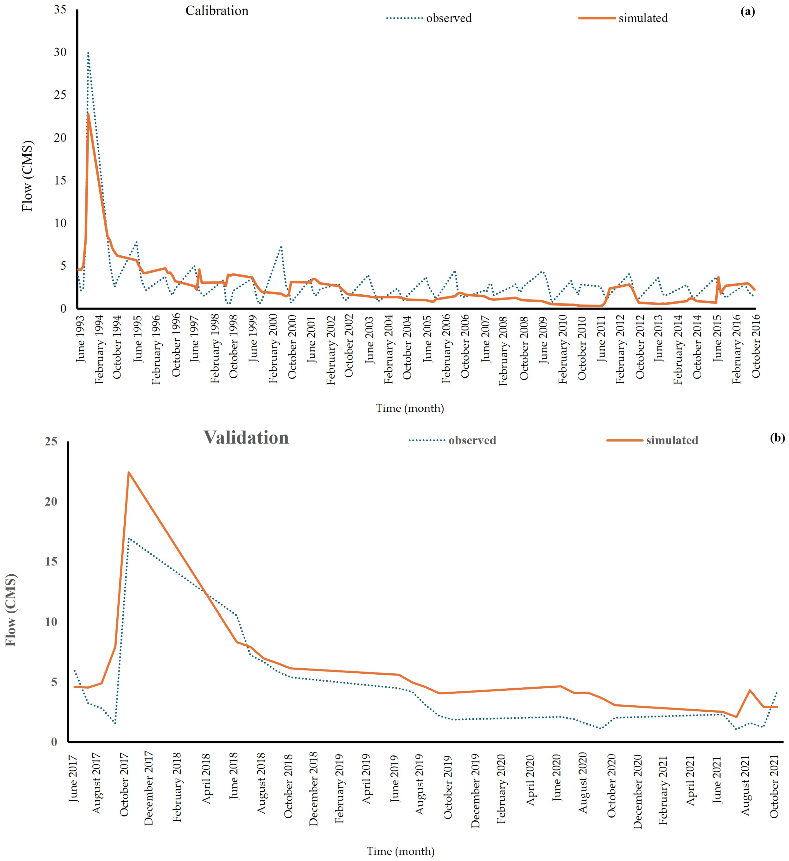
| A | 0.14 | 0.00 | 0.28 | 0.32 | - | - | - | - |
| B | 0.13 | 0.07 | 0.6 | 0.61 | 0.12 | 0.06 | 0.56 | 0.78 |
Disclaimer/Publisher’s Note: The statements, opinions and data contained in all publications are solely those of the individual author(s) and contributor(s) and not of MDPI and/or the editor(s). MDPI and/or the editor(s) disclaim responsibility for any injury to people or property resulting from any ideas, methods, instructions or products referred to in the content. |
© 2025 by the authors. Licensee MDPI, Basel, Switzerland. This article is an open access article distributed under the terms and conditions of the Creative Commons Attribution (CC BY) license (https://creativecommons.org/licenses/by/4.0/).
Share and Cite
Sabzevari, Y.; Eslamian, S.; Okhravi, S.; Bazrkar, M.H. Evaluating the Performance of Soil and Water Assessment Tool (SWAT) in a Snow-Dominated Climate (Case Study: Azna–Aligoudarz Basin, Iran). Atmosphere 2025, 16, 382. https://doi.org/10.3390/atmos16040382
Sabzevari Y, Eslamian S, Okhravi S, Bazrkar MH. Evaluating the Performance of Soil and Water Assessment Tool (SWAT) in a Snow-Dominated Climate (Case Study: Azna–Aligoudarz Basin, Iran). Atmosphere. 2025; 16(4):382. https://doi.org/10.3390/atmos16040382
Chicago/Turabian StyleSabzevari, Yaser, Saeid Eslamian, Saeid Okhravi, and Mohammad Hadi Bazrkar. 2025. "Evaluating the Performance of Soil and Water Assessment Tool (SWAT) in a Snow-Dominated Climate (Case Study: Azna–Aligoudarz Basin, Iran)" Atmosphere 16, no. 4: 382. https://doi.org/10.3390/atmos16040382
APA StyleSabzevari, Y., Eslamian, S., Okhravi, S., & Bazrkar, M. H. (2025). Evaluating the Performance of Soil and Water Assessment Tool (SWAT) in a Snow-Dominated Climate (Case Study: Azna–Aligoudarz Basin, Iran). Atmosphere, 16(4), 382. https://doi.org/10.3390/atmos16040382