
Interaction Between Maximum Entropies of Urban Meteorology and Pollutants: Effects on Relative Humidity and Temperature in the Boundary Layer of a Basin Geomorphology


Abstract
1. Introduction
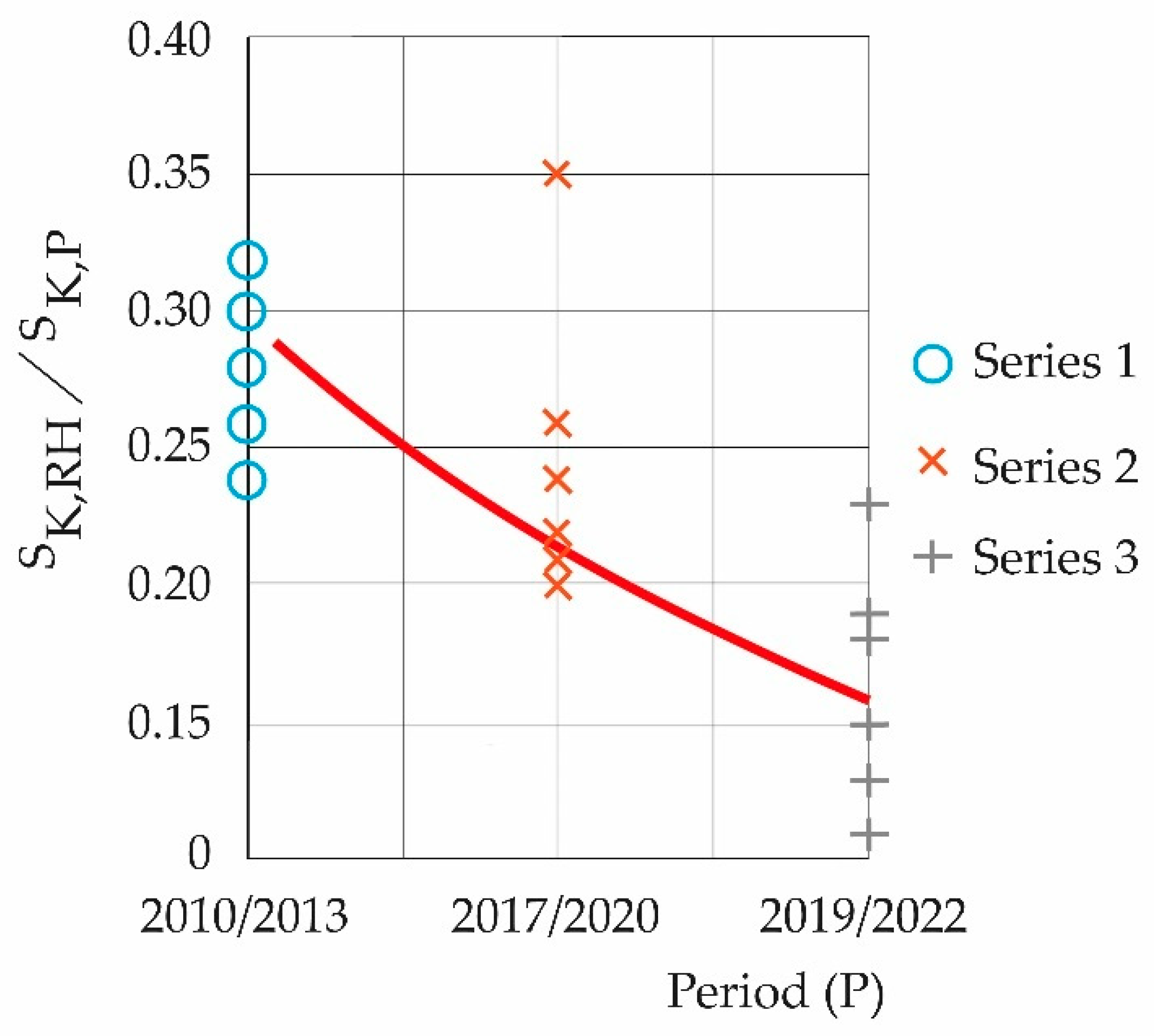
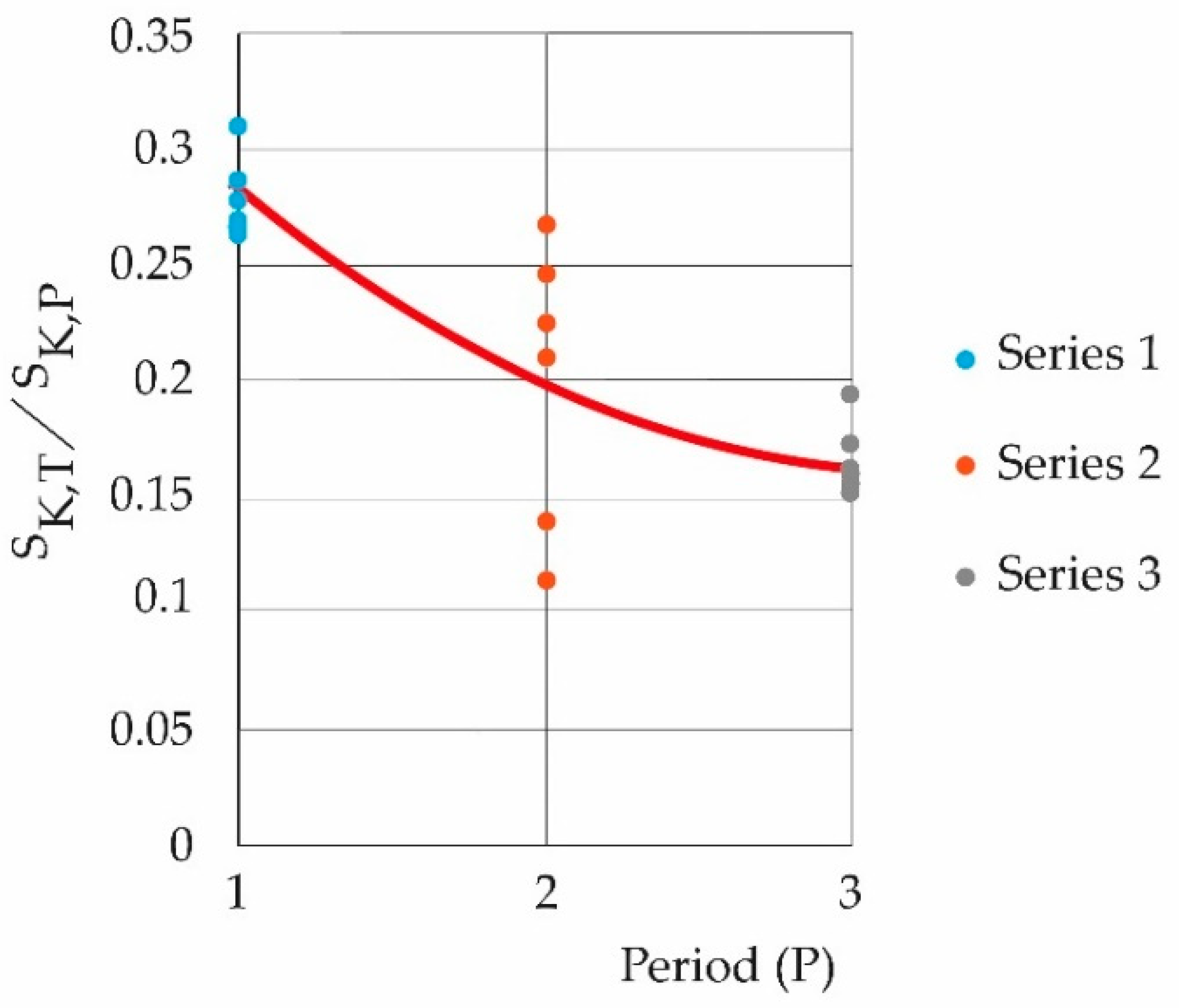
- The interactive decay, as the periods advance toward the present, of the quotient. This decay is compatible with what has been observed (of the relative humidity with respect to the pollutants and of the temperature with respect to the thermal flow of the pollutants).
- The presence of entropic dynamic
- The manifestation and permanence of a subdiffusive phenomenon in the studied basin.
- The presence of statistics of extreme events through the heavy-tail analysis.
1.1. Basic Concepts
1.1.1. Water in the Atmosphere
1.1.2. Atmospheric Composition
1.1.3. Pollution
1.1.4. Climate Change and Atmospheric Water
1.1.5. Relative Humidity (RH)
1.1.6. Thermodynamic Aspects Associated with Relative Humidity
Thermodynamic Principles
Latent Heat
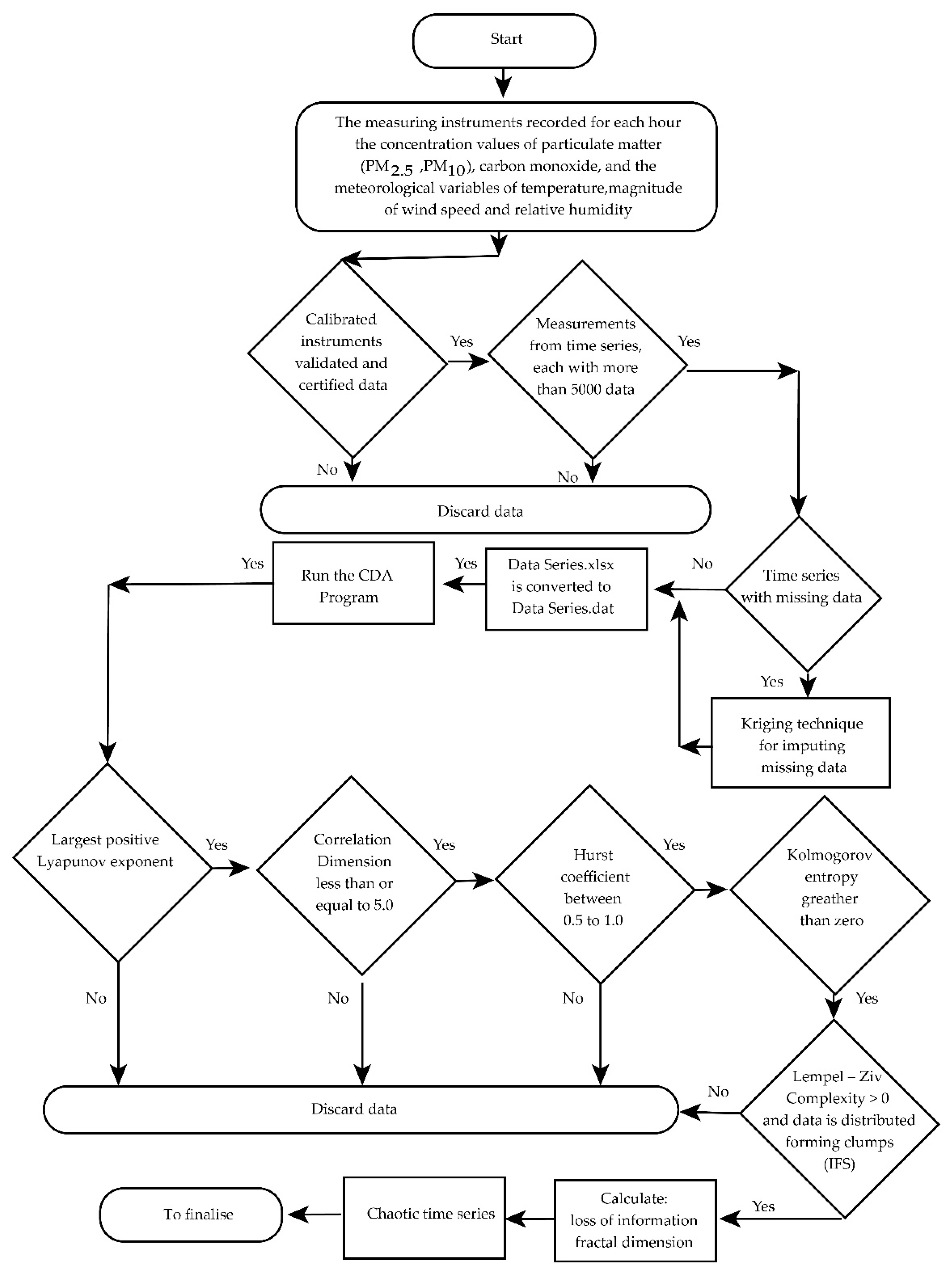
2. Materials and Methods
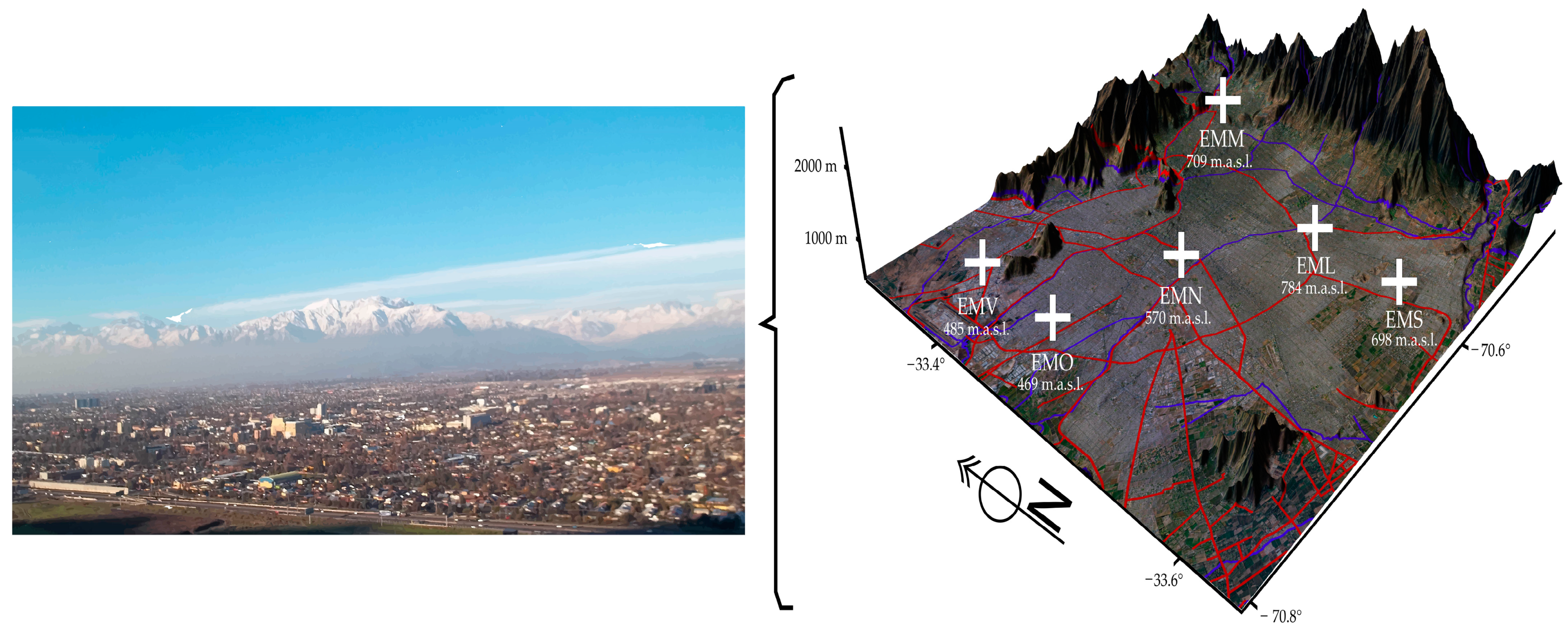
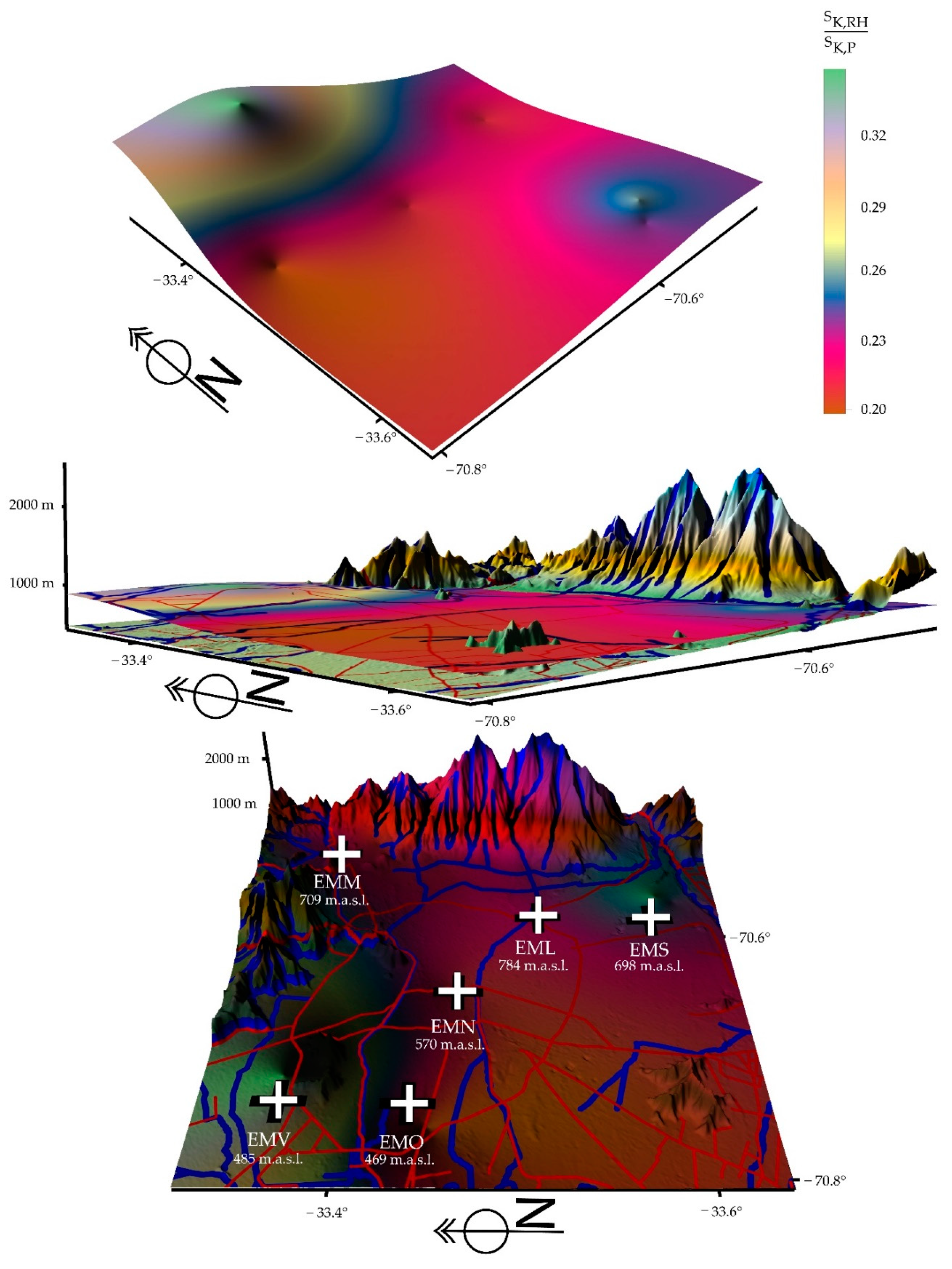
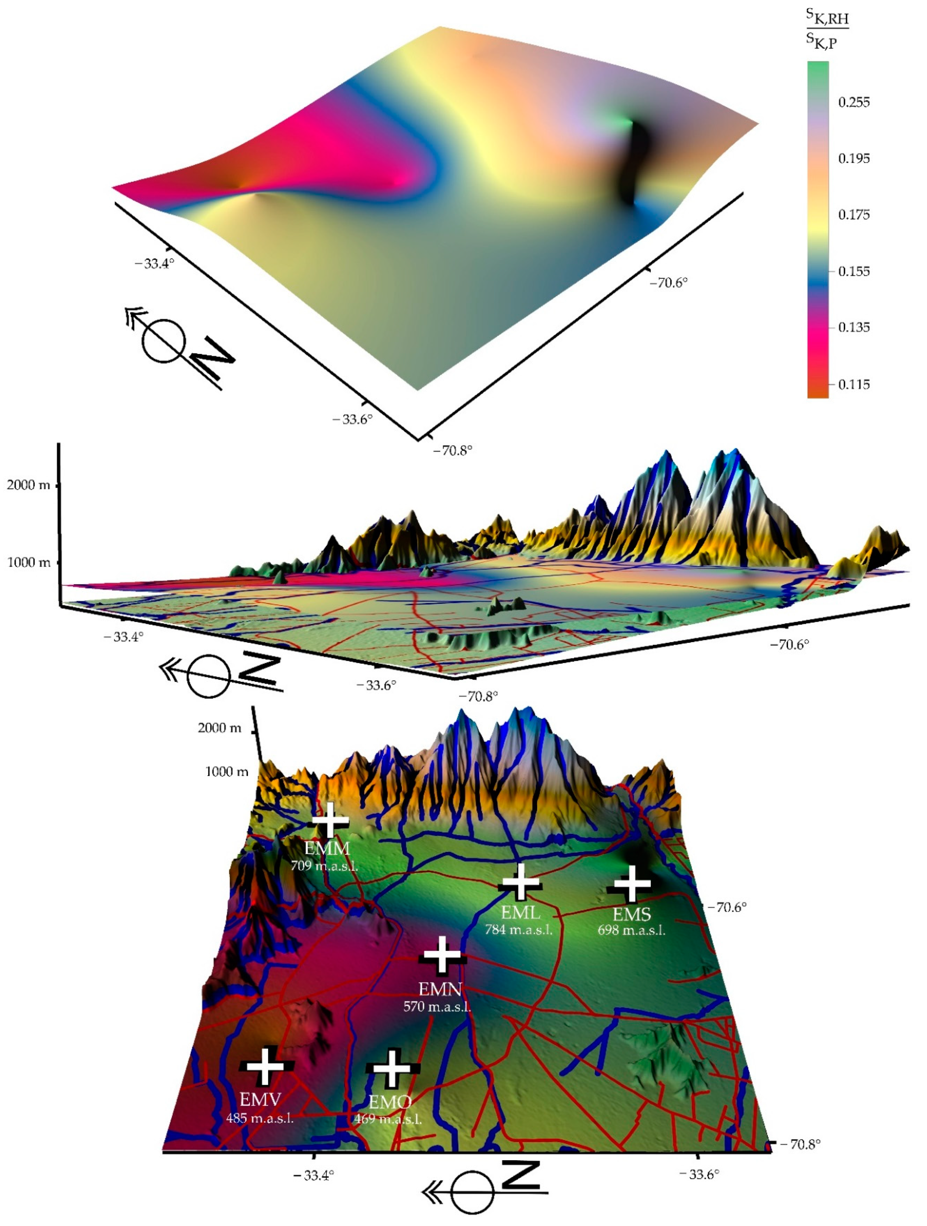
2.1. Study Area
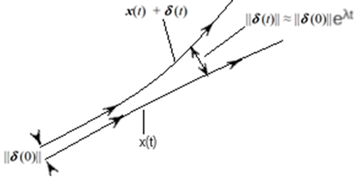
2.2. Kolmogorov Entropy
3. Results
3.1. Temperatures
3.2. Entropies
3.3. Thermal Fluxes
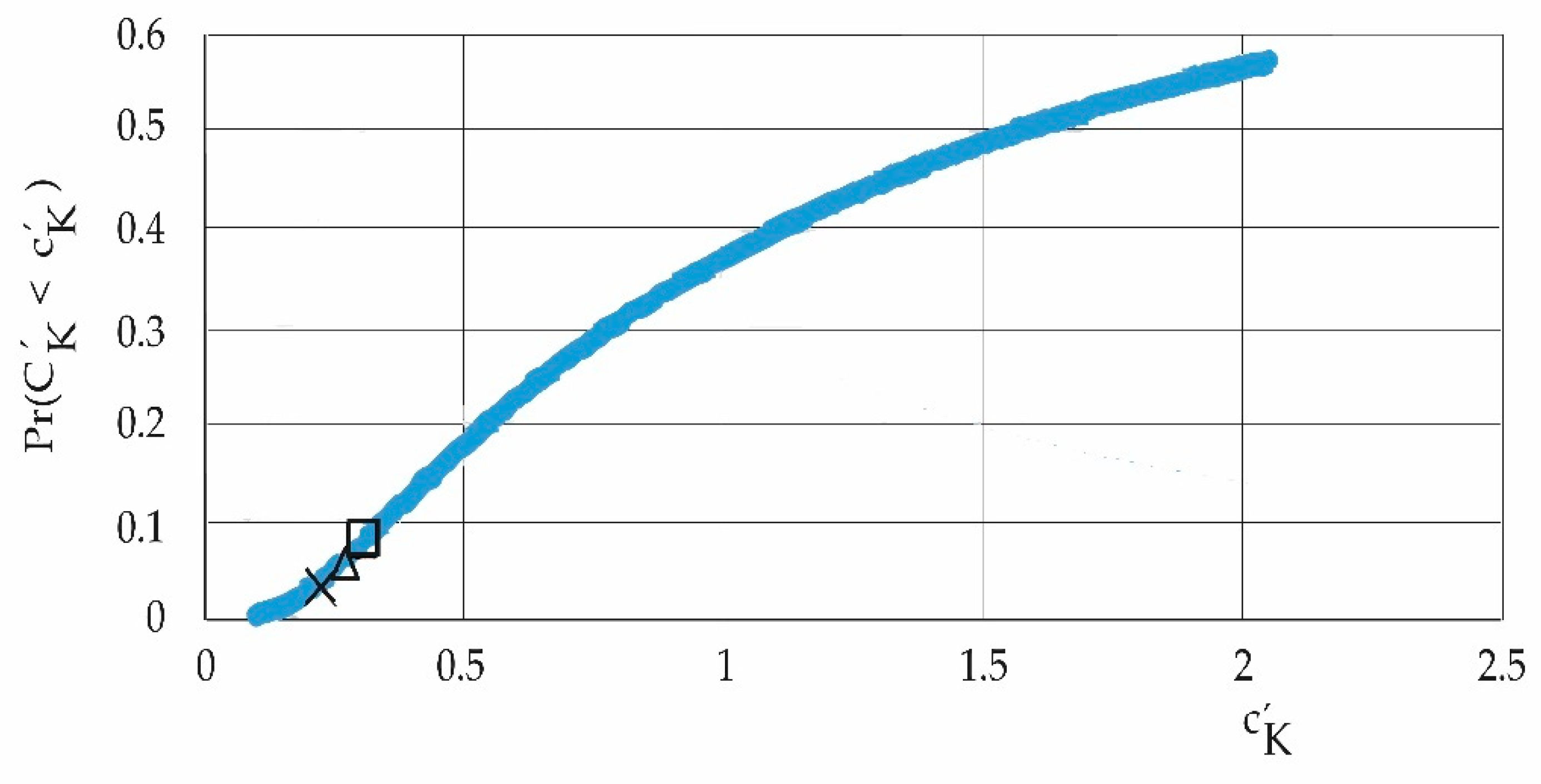
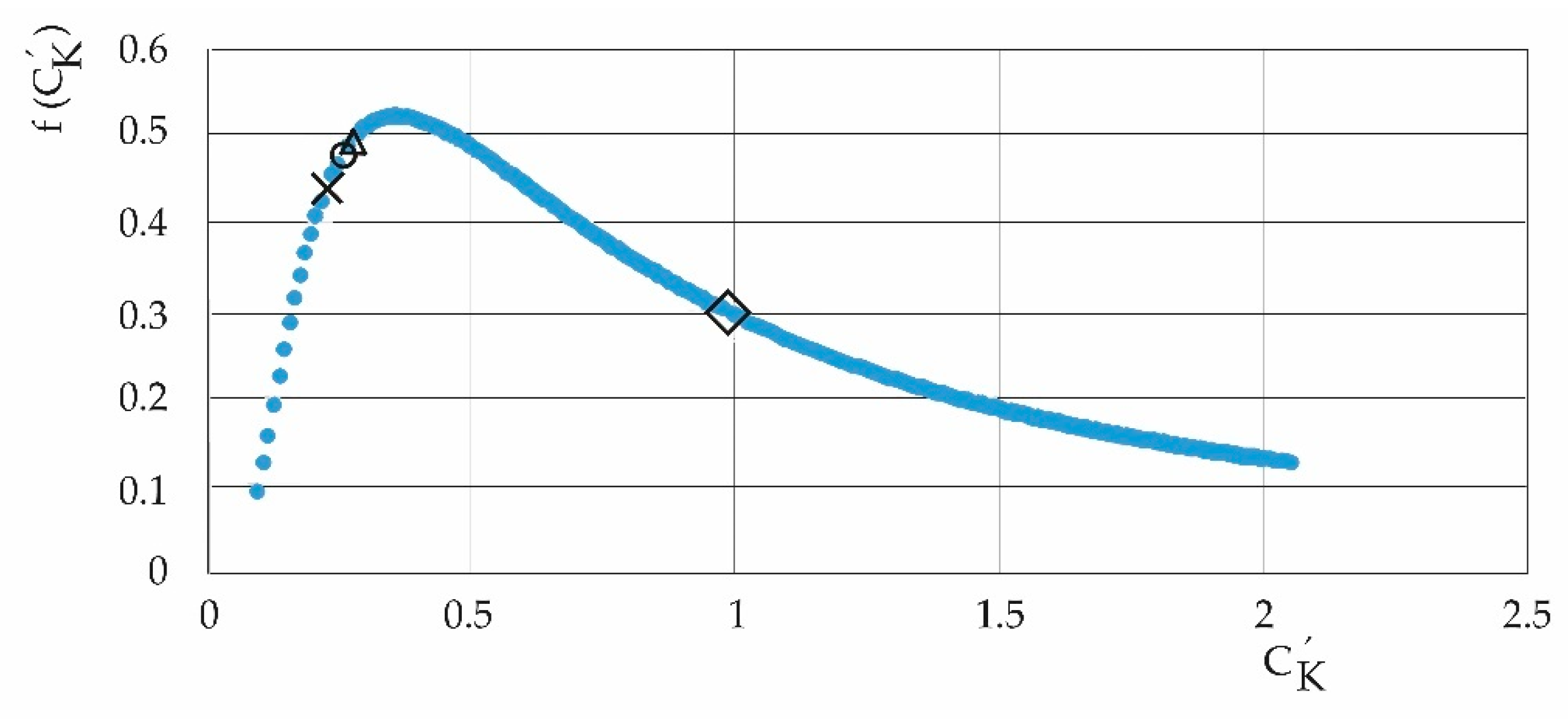
3.4. Anomalous Diffusion
- 1.
- 0 < c′K = SK,RH/SK,P <
- 2.
- 0 ≤ 1/c′K = SK,P/SK,RH <
4. Discussion
5. Conclusions
- The interactive decay, as the periods advance toward the present, of the quotient. This decay is compatible with what has been observed (of the relative humidity with respect to the pollutants and of the temperature with respect to the thermal flow of the pollutants).
- The presence of entropic dynamics associated with relative humidity and temperature, of lesser magnitude than those caused by pollutants.
- The manifestation and permanence of a subdiffusive phenomenon in the studied basin.
- The presence of statistics of extreme events through the heavy-tail analysis.
- In the number of pollutants considered, although they are most significant in the geomorphology of the studied basin;
- In which it is necessary to consider a fourth period of measurements of 3.25 years (2025/2028), which is currently being carried out, together with new measurements, in the same studied communities, using ultrasonic anemometers with the purpose of measuring the vertical component of the wind and the sonic temperature and carrying out comparative studies, during the interperiod, of thermal flows;
- Analyze the mountainous and coastal geomorphologies where the authors [22] have already carried out a follow-up showing that, in a first approximation, they seem to favor anomalous superdiffusion and heavy-tailed extreme events to the benefit of urban meteorology.
Author Contributions
Funding
Institutional Review Board Statement
Informed Consent Statement
Data Availability Statement
Acknowledgments
Conflicts of Interest
Appendix A

| Parameters Station | PM10 (µg/m3) | PM2.5 (µg/m3) | CO (ppm) | Temperature (°C) | RH (%) | WS (m/s) |
|---|---|---|---|---|---|---|
| EML | ||||||
| λ | 0.491 | 0.603 | 0.514 | 0.440 | 0.613 | 0.777 |
| Dc | 4.149 | 4.226 | 3.950 | 2.683 | 3.135 | 4.470 |
| H | 0.967 | 0.973 | 0.959 | 0.989 | 0.991 | 0.976 |
| SK (1/h) | 0.520 | 0.465 | 0.557 | 0.409 | 0.425 | 0.500 |
| EMM | ||||||
| λ | 0.302 | 0.585 | 0.630 | 0.460 | 0.713 | 0.892 |
| Dc | 3.877 | 3.966 | 4.719 | 3.128 | 3.507 | 4.285 |
| H | 0.972 | 0.977 | 0.981 | 0.991 | 0.990 | 0.980 |
| SK (1/h) | 0.441 | 0.528 | 0.581 | 0.409 | 0.427 | 0.616 |
| EMN | ||||||
| λ | 0.576 | 0.467 | 0.323 | 0.501 | 0.679 | 0.734 |
| Dc | 3.952 | 4.019 | 4.332 | 2.951 | 3.496 | 4.239 |
| H | 0.972 | 0.974 | 0.953 | 0.989 | 0.991 | 0.968 |
| SK (1/h) | 0.463 | 0.545 | 0.523 | 0.426 | 0.366 | 0.470 |
| EMO | ||||||
| λ | 0.467 | 0.289 | 0.229 | 0.453 | 0.689 | 0.855 |
| Dc | 3.785 | 4.085 | 4.640 | 2.801 | 3.194 | 4.053 |
| H | 0.965 | 0.955 | 0.937 | 0.992 | 0.989 | 0.968 |
| SK (1/h) | 0.522 | 0.428 | 0.260 | 0.375 | 0.382 | 0.440 |
| EMS | ||||||
| λ | 0.421 | 0.542 | 0.439 | 0.489 | 0.725 | 0.880 |
| Dc | 4.133 | 4.012 | 4.686 | 3.171 | 3.697 | 4.250 |
| H | 0.969 | 0.973 | 0.953 | 0.990 | 0.992 | 0.957 |
| SK (1/h) | 0.452 | 0.531 | 0.394 | 0.395 | 0.416 | 0.478 |
| EMV | ||||||
| λ | 0.561 | 0.295 | 0.296 | 0.495 | 0.746 | 0.836 |
| Dc | 3.788 | 3.788 | 4.631 | 3.155 | 3.249 | 3.584 |
| H | 0.967 | 0.970 | 0.952 | 0.989 | 0.989 | 0.956 |
| SK (1/h) | 0.552 | 0.538 | 0.341 | 0.384 | 0.370 | 0.448 |
| Parameters Station | PM10 (µg/m3) | PM2.5 (µg/m3) | CO (ppm) | Temperature (°C) | HR (%) | WV (m/s) |
|---|---|---|---|---|---|---|
| EML | ||||||
| λ | 0.550 | 0.235 | 0.026 | 0.205 | 0.064 | 0.935 |
| Dc | 3.451 | 1.364 | 0.580 | 2.290 | 2.029 | 3.697 |
| H | 0.922 | 0.963 | 0.933 | 0.915 | 0.942 | 0.975 |
| SK (1/h) | 0.295 | 0.596 | 0.686 | 0.355 | 0.414 | 0.515 |
| EMM | ||||||
| λ | 0.383 | 0.614 | 0.013 | 0.184 | 0.067 | 0.937 |
| Dc | 2.530 | 1.215 | 1.254 | 2.102 | 2.203 | 3.729 |
| H | 0.906 | 0.983 | 0.933 | 0.917 | 0.941 | 0.976 |
| SK (1/h) | 0.514 | 0.400 | 0.492 | 0.377 | 0.309 | 0.519 |
| EMN | ||||||
| λ | 0.621 | 0.292 | 0.033 | 0.223 | 0.092 | 0.917 |
| Dc | 2.948 | 1.276 | 2.277 | 2.280 | 2.095 | 3.735 |
| H | 0.929 | 0.960 | 0.933 | 0.916 | 0.942 | 0.973 |
| SK (1/h) | 0.242 | 0.825 | 0.412 | 0.366 | 0.308 | 0.471 |
| EMO | ||||||
| λ | 0.550 | 0.332 | 0.046 | 0.189 | 0.081 | 0.928 |
| Dc | 2.659 | 1.284 | 2.334 | 1.611 | 2.010 | 2.755 |
| H | 0.936 | 0.925 | 0.933 | 0.919 | 0.942 | 0.974 |
| SK (1/h) | 0.819 | 0.424 | 0.387 | 0.184 | 0.330 | 0.479 |
| EMS | ||||||
| λ | 0.597 | 0.279 | 0.030 | 0.228 | 0.063 | 0.933 |
| Dc | 3.535 | 1.396 | 3.302 | 2.300 | 2.306 | 3.004 |
| H | 0.921 | 0.975 | 0.933 | 0.915 | 0.942 | 0.976 |
| SK (1/h) | 0.898 | 0.422 | 0.382 | 0.357 | 0.404 | 0.489 |
| EMV | ||||||
| λ | 0.516 | 0.304 | 0.031 | 0.170 | 0.065 | 0.915 |
| Dc | 1.148 | 1.419 | 2.149 | 1.577 | 1.947 | 2.355 |
| H | 0.931 | 0.966 | 0.933 | 0.919 | 0.942 | 0.975 |
| SK (1/h) | 0.267 | 0.463 | 0.490 | 0.171 | 0.428 | 0.395 |
| Parameters Station | PM10 (µg/m3) | PM2.5 (µg/m3) | CO (ppm) | Temperature (°C) | HR (%) | WV(m/s) |
|---|---|---|---|---|---|---|
| EML | ||||||
| λ | 0.716 | 0.246 | 0.025 | 0.191 | 0.167 | 0.314 |
| Dc | 1.067 | 1.306 | 2.089 | 1.632 | 2.465 | 1.991 |
| H | 0.930 | 0.946 | 0.933 | 0.920 | 0.934 | 0.942 |
| SK (1/h) | 0.257 | 0.367 | 0.382 | 0.175 | 0.229 | 0.275 |
| EMM | ||||||
| λ | 0.561 | 0.345 | 0.011 | 0.220 | 0.203 | 0.339 |
| Dc | 0.984 | 1.531 | 2.156 | 1.923 | 2.691 | 1.986 |
| H | 0.914 | 0.969 | 0.933 | 0.916 | 0.935 | 0.942 |
| SK (1/h) | 0.247 | 0.360 | 0.333 | 0.182 | 0.180 | 0.278 |
| EMN | ||||||
| λ | 0.727 | 0.242 | 0.026 | 0.184 | 0.060 | 0.328 |
| Dc | 0.978 | 1.421 | 2.053 | 1.626 | 2.752 | 1.997 |
| H | 0.934 | 0.947 | 0.933 | 0.921 | 0.908 | 0.941 |
| SK (1/h) | 0.409 | 0.385 | 0.333 | 0.172 | 0.148 | 0.283 |
| EMO | ||||||
| λ | 0.540 | 0.332 | 0.015 | 0.222 | 0.256 | 0.347 |
| Dc | 0.973 | 1.354 | 2.095 | 1.821 | 2.499 | 2.019 |
| H | 0.940 | 0.920 | 0.933 | 0.918 | 0.936 | 0.941 |
| SK (1/h) | 0.388 | 0.400 | 0.329 | 0.180 | 0.205 | 0.283 |
| EMS | ||||||
| λ | 0.747 | 0.257 | 0.021 | 0.194 | 0.104 | 0.349 |
| Dc | 0.940 | 1.232 | 1.883 | 1.662 | 2.770 | 2.005 |
| H | 0.930 | 0.964 | 0.933 | 0.919 | 0.930 | 0.942 |
| SK (1/h) | 0.280 | 0.346 | 0.404 | 0.168 | 0.149 | 0.290 |
| EMV | ||||||
| λ | 0.574 | 0.241 | 0.580 | 0.161 | 0.714 | 0.080 |
| Dc | 0.945 | 1.432 | 2.127 | 1.559 | 2.704 | 1.939 |
| H | 0.930 | 0.938 | 0.933 | 0.920 | 0.934 | 0.940 |
| SK (1/h) | 0.252 | 0.415 | 0.285 | 0.153 | 0.100 | 0.351 |
Appendix B. [17]
References
- Selvam, A.M. Nonlinear Dynamics and Chaos: Applications in Meteorology and Atmospheric Physics. In Self-Organized Criticality and Predictability in Atmospheric Flows; Springer Atmospheric Sciences; Springer: Cham, Switzerland, 2017. [Google Scholar] [CrossRef]
- He, H.; Schäfer, B.; Beck, C. Spatial analysis of tails of air pollution PDFs in Europe. arXiv 2024. [Google Scholar] [CrossRef]
- Jizba, P.; Korbel, J. Maximum Entropy Principle in statistical inference: Case for non-Shannonian entropies. Phys. Rev. Lett. 2019, 22, 120601. [Google Scholar] [CrossRef] [PubMed]
- Tsallis, C.; Baldovin, F.; Cerbino, R.; Pierobon, P. Introduction to Nonextensive Statistical Mechanics and Thermodynamics. arXiv 2003. [Google Scholar] [CrossRef]
- Seidel, D.J.; Ao, C. 0.; Li, K. Estimating climatological planetary boundary layer heights from radiosonde observations: Comparison of methods and uncertainty analysis. J. Geophys. Res. Atmos. 2010, 115. [Google Scholar] [CrossRef]
- Quante, M.; Matthias, V. Water in the Earth’s atmosphere. J. Phys. IV France 2006, 139, 37–61. [Google Scholar] [CrossRef]
- Stull, R.B. Introduction to Boundary Layer Meteorology; Kluwer Academic Publishers: Dordrecht, The Netherlands; London, UK, 1988; p. 666. [Google Scholar]
- Schlesinger, W.H.; Bernhardt, E.S. The Atmosphere. In Biogeochemistry; Academic Press: Cambridge, MA, USA, 2020; pp. 51–97. [Google Scholar] [CrossRef]
- Meran, G.; Siehlow, M.; von Hirschhausen, C. Water Availability: A Hydrological View. In The Economics of Water; Springer Water; Springer: Cham, Switzerland, 2021. [Google Scholar] [CrossRef]
- Shiklomanov, I.A. World fresh water resources. In Water in Crisis: A Guide to the World’s Fresh Water Resources; Gleick, P.H., Ed.; Oxford University Press: New York, NY, USA, 1990; pp. 13–24. [Google Scholar]
- Wang, R.; Cui, K.; Sheu, H.L.; Wang, L.C.; Liu, X. Effects of Precipitation on the Air Quality Index, PM2.5 Levels and on the Dry Deposition of PCDD/Fs in the Ambient Air. Aerosol Air Qual. Res. 2023, 23, 220417. [Google Scholar] [CrossRef]
- Pacheco, P.R.; Salini, G.A.; Mera, E.M. Entropía y neguentropía: Una aproximación al proceso de difusión de contaminantes y su sostenibilidad. Rev. Int. Contam. Ambient. 2021, 37, 167–185. [Google Scholar] [CrossRef]
- Abbass, K.; Qasim, M.Z.; Song, H.; Murshed, M.; Mahmood, H.; Younis, I. A review of the global climate change impacts, adaptation, and sustainable mitigation measures. Environ. Sci. Pollut. Res. 2022, 29, 42539–42559. [Google Scholar] [CrossRef]
- Konapala, G.; Mishra, A.K.; Wada, Y.; Mann, M.E. Climate change will affect global water availability through compounding changes in seasonal precipitation and evaporation. Nat. Commun. 2020, 11, 3044. [Google Scholar] [CrossRef]
- Arnell, N.W. Climate change and global water resources. Glob. Environ. Change 1999, 91, S31–S49. [Google Scholar] [CrossRef]
- Patel, V.K.; Kuttippurath, J. Increase in Tropospheric Water Vapor Amplifies Global Warming and Climate Change. Ocean Land Atmos Res. 2023, 2, 0015. [Google Scholar] [CrossRef]
- Houghton, J.T.; Ding, Y.; Griggs, D.J.; Noguer, M.; van der Linden, P.J.; Dai, X. (Eds.) Climate Change 2001: The Scientific Basis, Contribution of Working Group I to the Third Assessment Report of the Intergovernmental Panel on Climate Change (IPCC); Cambridge University Press: Cambridge, UK, 2002; p. 944. [Google Scholar]
- Davis, R.E.; McGregor, G.R.; Enfield, K.B. Humidity: A review and primer on atmospheric moisture and human health. Environ. Res. 2016, 144, 106–116. [Google Scholar] [CrossRef] [PubMed]
- Guarnieri, G.; Olivieri, B.; Senna, G.; Vianello, A. Relative Humidity and Its Impact on the Immune System and Infections. Int. J. Mol. Sci. 2023, 24, 9456. [Google Scholar] [CrossRef] [PubMed]
- Wei, Q.; Xu, J.; Liao, L.; Yu, Y.; Liu, W.; Zhou, J.; Ding, Y. Indicators for evaluating trends of air humidification in arid regions under circumstance of climate change: Relative humidity (RH) vs. Actual water vapour pressure (ea). Ecol. Indic. 2021, 121, 107043. [Google Scholar] [CrossRef]
- Peixoto, J.; Oort, A.H. 1996: The Climatology of Relative Humidity in the Atmosphere. J. Clim. 1996, 9, 3443–3463. [Google Scholar] [CrossRef]
- Pacheco, P.; Mera, E.; Navarro, G.; Parodi, C. Urban Meteorology, Pollutants, Geomorphology, Fractality, and Anomalous Diffusion. Fractal Fract. 2024, 8, 204. [Google Scholar] [CrossRef]
- Verlinde, E. On the Origin of Gravity and the Laws of Newton. arXiv 2010. [Google Scholar] [CrossRef]
- Peterson, M.A. Analogy between thermodynamics and mechanics. Am. J. Phys. 1979, 47, 488. [Google Scholar] [CrossRef]
- Baldiotti, M.C.; Fresneda, R.; Molina, C. A Hamiltonian approach to Thermodynamics. Ann. Phys. 2016, 373, 245–256. [Google Scholar] [CrossRef]
- Mao, Y.; Li, Y.; Yuan, X.; Kosonen, R. Characterization of the maximum entropy change in the process of drying materials based on a heat pump. Therm. Sci. Eng. Prog. 2024, 47, 102292, ISSN 2451-9049. [Google Scholar] [CrossRef]
- Zeng, X.; Tao, W.-K.; Simpson, J. An Equation for Moist Entropy in a Precipitating and Icy Atmosphere. J. Atmos. Sci. 2005, 62, 4293–4309. [Google Scholar] [CrossRef]
- Pikeroen, Q.; Paillard, D.; Watrin, K. A radiative–convective model computing precipitation with the maximum entropy production hypothesis. Geosci. Model Dev. 2024, 17, 3801–3814. [Google Scholar] [CrossRef]
- Li, J.; Chylek, P. Atmospheric Entropy. Part I: Climate Dissipation Structure. J. Clim. 2012, 25, 3173–3190. [Google Scholar] [CrossRef]
- Kleidon, A. Entropy Production by Evapotranspiration and its Geographic Variation. Soil Water Res. 2008, 3, S89–S94. [Google Scholar] [CrossRef]
- Alahmer, A.; Omar, M.A.; Mayyas, A.; Dongri, S. Effect of relative humidity and temperature control on in-cabin thermal comfort state: Thermodynamic and psychometric analyses. Appl. Therm. Eng. 2011, 31, 2636–2644. [Google Scholar] [CrossRef]
- Boregowda, S.C.; Choate, R.E.; Handy, R. Entropy Generation Analysis of Human Thermal Stress Responses. Int. Sch. Res. Netw. ISRN Thermodyn. 2012, 2012, 830103. [Google Scholar] [CrossRef]
- Mendoza, V.; Pazos, M.; Garduño, R.; Mendoza, B. Thermodynamics of climate change between cloud cover, atmospheric temperature and humidity. Sci. Rep. 2021, 11, 21244. [Google Scholar] [CrossRef]
- London, J.A. Study of the Atmospheric Heat Balance; New York University: New York, NY, USA, 1957. [Google Scholar]
- Sprott, J.C. Chaos and Time-Series Analysis, 1st ed.; Oxford University Press: Oxford, UK, 2003. [Google Scholar]
- Sprott, J.C. Chaos Data Analyzer Software. The Professional Version 2.1, 1998, Madison Wisconsin, USA. Available online: http://sprott.physics.wisc.edu/cda.htm (accessed on 12 November 2024).
- Pacheco, P.; Mera, E.; Salini, G. Urban Densification Effect on Micrometeorology in Santiago, Chile: A Comparative Study Based on Chaos Theory. Sustainability 2022, 14, 2845. [Google Scholar] [CrossRef]
- Shiozawa, K.; Tokuda, I.S. Estimating Kolmogorov–Sinai entropy from time series of high-dimensional complex systems. Phys. Lett. A 2024, 510, 129531. [Google Scholar] [CrossRef]
- Farmer, J.D. Chaotic attractors of an infinite dimensional dynamical system. Phys. D 1982, 4, 366–393. [Google Scholar] [CrossRef]
- Farmer, J.D.; Otto, E.; Yorke, J.A. The dimension of chaotic attractors. Phys. D 1983, 7, 153–180. [Google Scholar] [CrossRef]
- Farmer, J.D. Information Dimension and the Probabilistic Structure of Chaos. Z. Für Naturforschung A 1982, 37, 1304–1326. [Google Scholar] [CrossRef]
- Shannon, C. A mathematical theory of communication. Bell Syst. Tech. 1948, 27, 379–423. [Google Scholar] [CrossRef]
- Kolmogorov, A.N. On Entropy per unit Time as a Metric Invariant of Automorphisms. Dokl. Akad. Nauk. SSSR 1959, 124, 754–755. [Google Scholar]
- Sinai, Y.G. On the concept of entropy of a dynamical system. Dolk. Akad. Nauk. SSSR 1959, 124, 768. [Google Scholar]
- Pesin, Y. Characteristic Lyapunov exponents and smooth ergodic theory. Russ. Math. Surv. 1977, 32, 55–114. [Google Scholar] [CrossRef]
- Ruelle, D. Thermodynamic Formalism; Addison-Wesley-Longman: Reading, MA, USA, 1978. [Google Scholar]
- Wolf, A.; Swift, J.B.; Swinney, H.L.; Vastano, J.A. Determining Lyapunov exponents from a time series. Phys. D 1985, 16, 285–317. [Google Scholar] [CrossRef]
- Pacheco, P.; Mera, E.; Fuentes, V. Intensive Urbanization, Urban Meteorology and Air Pollutants: Effects on the Temperature of a City in a Basin Geography. Int. J. Environ. Res. Public Health 2023, 20, 3941. [Google Scholar] [CrossRef]
- Middelburg, J.J. The Gibbs Free Energy. In Thermodynamics and Equilibria in Earth System Sciences: An Introduction; SpringerBriefs in Earth System Sciences; Springer: Cham, Switzerland, 2024. [Google Scholar] [CrossRef]
- Fréchet, M. Sur la loi de probabilité de l’écart maximum. Ann. Société Pol. Math. Crac. 1927, 6, 93–116. [Google Scholar]
- Fisher, R.A.; Tippett, L.H.C. Limiting forms of the frequency distribution of the largest or smallest member of a sample. Math. Proc. Camb. Philos. Soc. 1928, 24, 180–190. [Google Scholar] [CrossRef]
- Pacheco, P.; Mera, E. Evolution over Time of Urban Thermal Conditions of a City Immersed in a Basin Geography and Mitigation. Atmosphere 2023, 14, 777. [Google Scholar] [CrossRef]
- Cuthbert, M.O.; Rau, G.C.; Ekström, M.; O’carroll, D.M.; Bates, A.J. Global climate-driven trade-offs between the water retention and cooling benefits of urban greening. Nat. Commun. 2022, 13, 518. [Google Scholar] [CrossRef]
- Bolan, S.; Padhye, L.P.; Jasemizad, T.; Govarthanan, M.; Karmegam, N.; Wijesekara, H.; Amarasiri, D.; Hou, D.; Zhou, P.; Biswal, B.K.; et al. Impacts of climate change on the fate of contaminants through extreme weather events. Sci. Total Environ. 2024, 909, 168388. [Google Scholar] [CrossRef] [PubMed]
- Russo, S.; Sillmann, J.; Sterl, A. Humid heat waves at different warming levels. Sci. Rep. 2017, 7, 7477. [Google Scholar] [CrossRef]
- Robinson, P.J. On the Definition of a Heat Wave. J. Appl. Meteor. Climatol. 2001, 40, 762–775. [Google Scholar] [CrossRef]
- Pacheco, P.; Mera, E.; Navarro, G. The Effects of Lockdown, Urban Meteorology, Pollutants, and Anomalous Diffusion on the SARS-CoV-2 Pandemic in Santiago de Chile. Atmosphere 2024, 15, 414. [Google Scholar] [CrossRef]
- Swain, D.L.; Prein, A.F.; Abatzoglou, J.T.; Albano, C.M.; Brunner, M.; Diffenbaugh, N.S.; Singh, D.; Skinner, C.B.; Touma, D. Hydroclimate volatility on a warming Earth. Nat. Rev. Earth Environ. 2025, 6, 35–50. [Google Scholar] [CrossRef]


| EML | EMM | EMV | EMN | EMS | EMO | Average by Commune | |
|---|---|---|---|---|---|---|---|
| 2010–2013 | |||||||
| (°C) | 15.4 | 15.86 | 15.80 | 15.34 | 14.70 | 16.80 | 15.65 |
| (%) | 58.20 | 58.13 | 57.34 | 60.22 | 60.07 | 57.52 | 58.58 |
| 2017–2020 | |||||||
| (°C) | 16.12 | 15.57 | 16.85 | 16.17 | 15.53 | 16.78 | 16.17 |
| (%) | 55.31 | 55.00 | 58.95 | 57.31 | 56.07 | 59.22 | 56.98 |
| 2019–2022 | |||||||
| (°C) | 16.10 | 14.70 | 15.50 | 16.05 | 15.42 | 15.31 | 15.51 |
| (%) | 56.20 | 57.83 | 61.20 | 60.84 | 56.96 | 61.32 | 59.10 |
| PM10 | PM2.5 | CO | T | HR | WV | ||
|---|---|---|---|---|---|---|---|
| EML | 2010–2013 | ||||||
| H | 0.967 | 0.973 | 0.959 | 0.989 | 0.991 | 0.976 | |
| D | 1.033 | 1.027 | 1.041 | 1.011 | 1.009 | 1.024 | |
| 2017–2020 | |||||||
| H | 0.922 | 0.963 | 0.933 | 0.915 | 0.942 | 0.975 | |
| D | 1.078 | 1.037 | 1.067 | 1.085 | 1.058 | 1.025 | |
| 2019–2022 | |||||||
| H | 0.928 | 0.946 | 0.933 | 0.920 | 0.934 | 0.942 | |
| D | 1.072 | 1.054 | 1.067 | 1.080 | 1.066 | 1.058 | |
| EMM | 2010–2013 | ||||||
| H | 0.972 | 0.977 | 0.981 | 0.991 | 0.990 | 0.980 | |
| D | 1.028 | 1.023 | 1.019 | 1.009 | 1.010 | 1.02 | |
| 2017–2020 | |||||||
| H | 0.906 | 0.983 | 0.933 | 0.917 | 0.941 | 0.976 | |
| D | 1.094 | 1.017 | 1.067 | 1.083 | 1.059 | 1.024 | |
| 2019–2022 | |||||||
| H | 0.914 | 0.969 | 0.933 | 0.916 | 0.935 | 0.942 | |
| D | 1.086 | 1.031 | 1.067 | 1.084 | 1.065 | 1.058 | |
| EMN | 2010–2013 | ||||||
| H | 0.972 | 0.974 | 0.953 | 0.989 | 0.991 | 0.968 | |
| D | 1.028 | 1.026 | 1.047 | 1.011 | 1.009 | 1.032 | |
| 2017–2020 | |||||||
| H | 0.929 | 0.960 | 0.933 | 0.916 | 0.942 | 0.973 | |
| D | 1.071 | 1.040 | 1.067 | 1.084 | 1.058 | 1.027 | |
| 2019–2022 | |||||||
| H | 0.934 | 0.947 | 0.933 | 0.921 | 0.908 | 0.941 | |
| D | 1.066 | 1.053 | 1.067 | 1.079 | 1.092 | 1.059 | |
| EMO | 2010–2013 | ||||||
| H | 0.965 | 0.955 | 0.937 | 0.992 | 0.989 | 0.968 | |
| D | 1.035 | 1.045 | 1.063 | 1.008 | 1.011 | 1.032 | |
| 2017–2020 | |||||||
| H | 0.936 | 0.925 | 0.933 | 0.919 | 0.942 | 0.974 | |
| D | 1.064 | 1.075 | 1.067 | 1.081 | 1.058 | 1.026 | |
| 2019–2022 | |||||||
| H | 0.938 | 0.915 | 0.933 | 0.918 | 0.936 | 0.941 | |
| D | 1.062 | 1.085 | 1.067 | 1.082 | 1.064 | 1.059 | |
| EMS | 2010–2013 | ||||||
| H | 0.969 | 0.973 | 0.953 | 0.990 | 0.992 | 0.957 | |
| D | 1.031 | 1.027 | 1.047 | 1.010 | 1.008 | 1.043 | |
| 2017–2020 | |||||||
| H | 0.921 | 0.975 | 0.933 | 0.915 | 0.942 | 0.976 | |
| D | 1.079 | 1.025 | 1.067 | 1.085 | 1.058 | 1.024 | |
| 2019–2022 | |||||||
| H | 0.930 | 0.964 | 0.933 | 0.919 | 0.927 | 0.942 | |
| D | 1.070 | 1.036 | 1.067 | 1.081 | 1.073 | 1.058 | |
| EMV | 2010–2013 | ||||||
| H | 0.967 | 0.970 | 0.952 | 0.989 | 0.989 | 0.956 | |
| D | 1.033 | 1.03 | 1.048 | 1.011 | 1.011 | 1.044 | |
| 2017–2020 | |||||||
| H | 0.931 | 0.966 | 0.933 | 0.919 | 0.942 | 0.975 | |
| D | 1.069 | 1.034 | 1.067 | 1.081 | 1.058 | 1.025 | |
| 2019–2022 | |||||||
| H | 0.930 | 0.938 | 0.933 | 0.920 | 0.934 | 0.940 | |
| D | 1.070 | 1.062 | 1.067 | 1.080 | 1.066 | 1.060 |
| Station | EMS | EML | EMN | EMO | EMV | EMM |
|---|---|---|---|---|---|---|
| Average (°C/h) | −0.09113202 | −0.0680180 | −0.0092004 | 0.0206236 | 0. 00662203 | −0.10181307 |
| Addition (°C/h) | −2593.89069 | −1935.99887 | −261.870346 | 587.009455 | 453.866082 | −2897.90535 |
| Average (K/h) | 273.06 K/h | 273.08 K/h | 273.14 K/h | 273.17 K/h | 273.16 K/h | 273.08 K/h |
| Height (masl) | 485 | 784 | 520 | 469 | 698 | 709 |
| Station | H (masl) | (K/h)S1,2010–2013 | (K/h)S2,2017–2020 | (K/h)S3,2019–2022 | + Av (°C)2010–2013 | + Av (°C)2017–2020 | + Av (°C)2019–2022 |
|---|---|---|---|---|---|---|---|
| EML | 784 | 273.50 | 273.80 | 273.08 | 15.40 + 0.36 = 15.8 | 16.12 + 0.93 = 17.1 | 16.09 − 0.0680 = 16.02 |
| EMM * | 709 | 273.54 | 274.00 | 273.08 | 15.86 + 0.40 = 16.3 | 15.57 + 0.62 = 16.2 | 14.69 − 0.1018 = 14.60 |
| EMV | 698 | 273.60 | 274.10 | 273.16 | 15.77 + 0.50 = 16.3 | 16.85 + 0.66 = 17.5 | 15.50 + 0.0662 = 15.50 |
| EMN | 520 | 273.50 | 273.81 | 273.14 | 15.34 + 0.36 = 15.7 | 16.17 + 0.96 = 17.1 | 16.047 − 0.092 = 16.04 |
| EMS | 485 | 273.60 | 274.10 | 273.06 | 14.69 + 0.42 = 15.1 | 15.53 + 0.94 = 16.5 | 15.42 − 0.0911 = 15.33 |
| EMO | 469 | 273.80 | 274.10 | 273.17 | 16.77 + 0.60 = 17.4 | 16.80 + 0.80 = 17.6 | 15.31 + 0.0206 = 15.33 |
| Parameters Station | SK,P 2010/2013 | SK,HR 2010/2013 | SK,P 2017/2020 | SK,HR 2017/2020 | SK,P 2019/2022 | SK,HR 2019/2022 |
|---|---|---|---|---|---|---|
| EML | ||||||
| SK (1/h) | 1.542 | 0.425 | 1.577 | 0.414 | 1.006 | 0.229 |
| EMM | ||||||
| SK (1/h) | 1.550 | 0.427 | 1.406 | 0.309 | 0.940 | 0.180 |
| EMN | ||||||
| SK (1/h) | 1.531 | 0.366 | 1.479 | 0.308 | 1.127 | 0.148 |
| EMO | ||||||
| SK (1/h) | 1.210 | 0.382 | 1.630 | 0.330 | 1.117 | 0.205 |
| EMS | ||||||
| SK (1/h) | 1.377 | 0.416 | 1.702 | 0.404 | 1.030 | 0.149 |
| EMV | ||||||
| SK (1/h) | 1.431 | 0.370 | 1.220 | 0.428 | 0.952 | 0.100 |
| Parameters Station | SK,HR/SK,P 2010/2013 | SK,HR/SK,P 2017/2020 | SK,HR/SK,P 2019/2022 |
|---|---|---|---|
| EML | 0.28 | 0.26 | 0.23 |
| EMM | 0.28 | 0.22 | 0.19 |
| EMN | 0.24 | 0.21 | 0.13 |
| EMO | 0.32 | 0.20 | 0.18 |
| EMS | 0.30 | 0.24 | 0.15 |
| EMV | 0.26 | 0.35 | 0.11 |
| Parameters Station | SK,P 2010/2013 | SK,T 2010/2013 | SK,P 2017/2020 | SK,T 2017/2020 | SK,P 2019/2022 | SK,T 2019/2022 |
|---|---|---|---|---|---|---|
| EML | ||||||
| SK (1/h) | 1.542 | 0.409 | 1.577 | 0.355 | 1.006 | 0.175 |
| EMM | ||||||
| SK (1/h) | 1.550 | 0.409 | 1.406 | 0.377 | 0.940 | 0.182 |
| EMN | ||||||
| SK (1/h) | 1.531 | 0.426 | 1.479 | 0.366 | 1.127 | 0.172 |
| EMO | ||||||
| SK (1/h) | 1.210 | 0.375 | 1.630 | 0.184 | 1.117 | 0.180 |
| EMS | ||||||
| SK (1/h) | 1.377 | 0.395 | 1.702 | 0.357 | 1.030 | 0.168 |
| EMV | ||||||
| SK (1/h) | 1.431 | 0.384 | 1.220 | 0.171 | 0.952 | 0.153 |
| Parameters Station | SK,T/SK,P 2010/2013 | SK,T/SK,P 2017/2020 | SK,T/SK,P 2019/2022 |
|---|---|---|---|
| EML | 0.265 | 0.225 | 0.174 |
| EMM | 0.264 | 0.268 | 0.194 |
| EMN | 0.278 | 0.247 | 0.153 |
| EMO | 0.310 | 0.113 | 0.161 |
| EMS | 0.287 | 0.210 | 0.163 |
| EMV | 0.268 | 0.140 | 0.161 |
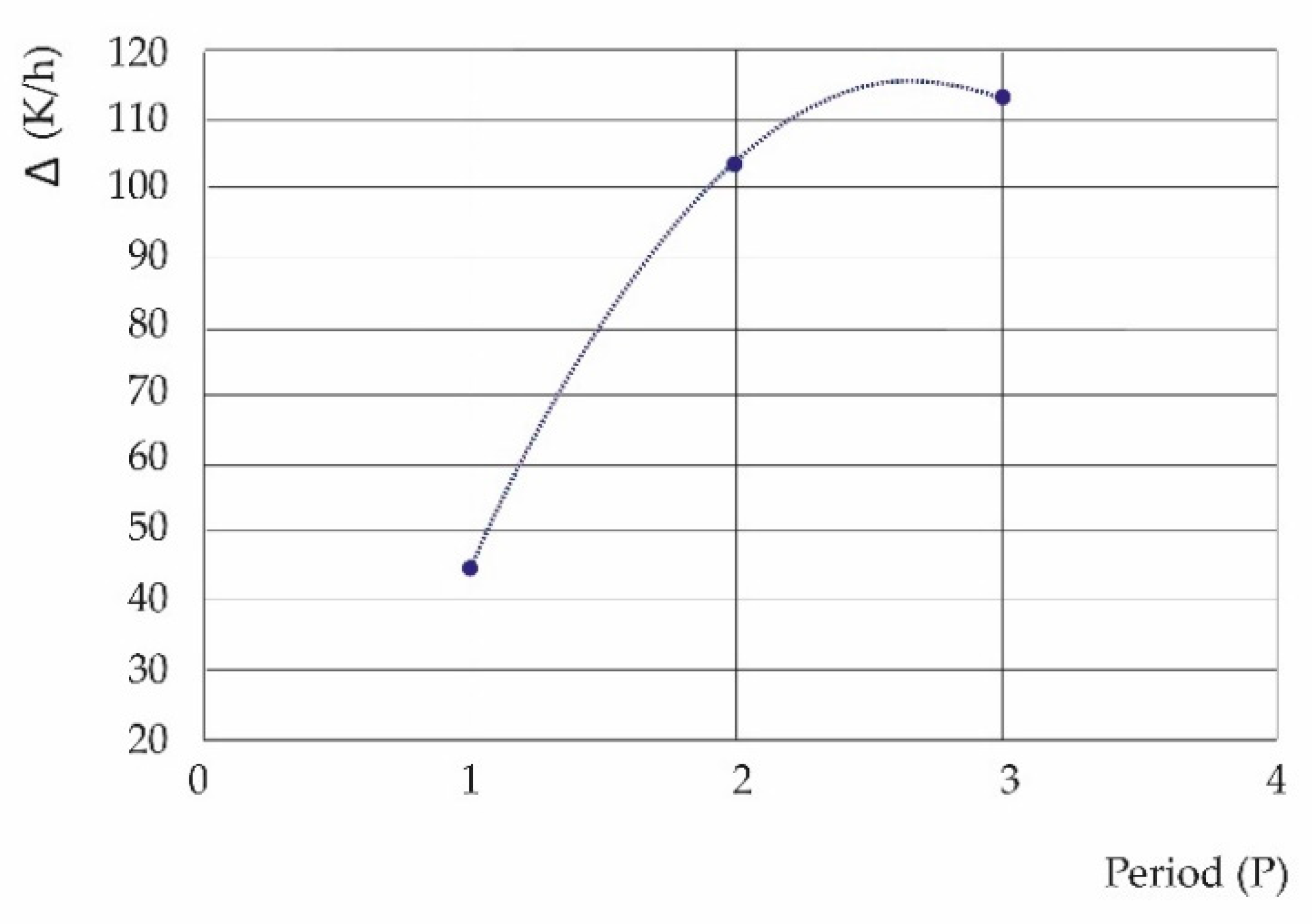
| h (masl) | (°C) | SKP (1/h) | SKMV (1/h) | (δQ/dt)P(K/h) | (δQ/dt)MV(K/h) | Δ(K/h) |
|---|---|---|---|---|---|---|
| 784 (EML) | 16.10 | 1.006 | 0.679 | 291.0000 | 196.4001 | 94.6000 |
| 709 (EMM) | 14.70 | 0.904 | 0.640 | 260.2164 | 184.2240 | 76.0000 |
| 698 (EMV) | 15.50 | 1.030 | 0.607 | 297.3095 | 175.2106 | 122.1000 |
| 520 (EMN) | 16.05 | 1.127 | 0.603 | 325.9284 | 174.3876 | 151.5408 |
| 485 (EMS) | 15.42 | 0.952 | 0.604 | 274.7186 | 174.2963 | 100.4223 |
| 469 (EMO) | 15.31 | 1.117 | 0.668 | 322.2098 | 192.6913 | 129.5185 |
| 15.51 | 295.2305 | 182.8683 | 112.3636 |
Disclaimer/Publisher’s Note: The statements, opinions and data contained in all publications are solely those of the individual author(s) and contributor(s) and not of MDPI and/or the editor(s). MDPI and/or the editor(s) disclaim responsibility for any injury to people or property resulting from any ideas, methods, instructions or products referred to in the content. |
© 2025 by the authors. Licensee MDPI, Basel, Switzerland. This article is an open access article distributed under the terms and conditions of the Creative Commons Attribution (CC BY) license (https://creativecommons.org/licenses/by/4.0/).
Share and Cite
Pacheco, P.; Mera, E.; Navarro, G.; Polo, S. Interaction Between Maximum Entropies of Urban Meteorology and Pollutants: Effects on Relative Humidity and Temperature in the Boundary Layer of a Basin Geomorphology. Atmosphere 2025, 16, 337. https://doi.org/10.3390/atmos16030337
Pacheco P, Mera E, Navarro G, Polo S. Interaction Between Maximum Entropies of Urban Meteorology and Pollutants: Effects on Relative Humidity and Temperature in the Boundary Layer of a Basin Geomorphology. Atmosphere. 2025; 16(3):337. https://doi.org/10.3390/atmos16030337
Chicago/Turabian StylePacheco, Patricio, Eduardo Mera, Gustavo Navarro, and Steicy Polo. 2025. "Interaction Between Maximum Entropies of Urban Meteorology and Pollutants: Effects on Relative Humidity and Temperature in the Boundary Layer of a Basin Geomorphology" Atmosphere 16, no. 3: 337. https://doi.org/10.3390/atmos16030337
APA StylePacheco, P., Mera, E., Navarro, G., & Polo, S. (2025). Interaction Between Maximum Entropies of Urban Meteorology and Pollutants: Effects on Relative Humidity and Temperature in the Boundary Layer of a Basin Geomorphology. Atmosphere, 16(3), 337. https://doi.org/10.3390/atmos16030337