Abstract
Various machine learning algorithms exist to predict air quality, but they can only analyse structured data gathered from monitoring stations. However, the concentration of certain pollutants, such as PM2.5 and PM10, can be visually significant when there is a marked difference in their levels. Consequently, air quality from meteorological cameras can be estimated and integrated with data from monitoring stations to generate an air quality forecast. This research delves into the prospect of creating a methodology capable of rapidly processing this information and producing precise air quality predictions using time series analytics. This paper presents a study of developing a new model, the “Convolutional Neural Network, Recurrent Neural Network Dual Input Model” (CORD). This model combines the convolutional neural network (CNN) and recurrent neural network (RNN) models that are applied to prediction to create an air pollution-related forecasting function to overcome the monitoring stations’ physical limitations. CORD is a model that allows for dual input types: structured data from air quality data collected with meteorological cameras and images (unstructured data) from monitoring stations. This prototype could be applied to all air quality indices worldwide, and CORD is tested based on the Air Quality Health Index provided by the Hong Kong Observatory, a unique data-analytic framework based on air quality measurement. CORD has a similar result to GRU and slightly smaller mean absolute and root mean square errors than LSTM. Compared with an ANN algorithm, CORD has better accuracy.
1. Introduction
Air pollution is a significant global concern, with adverse impacts on public health, the environment, and overall quality of life. Accurate and timely air quality prediction is essential for mitigating these effects, yet it remains a challenging task due to the complexity of atmospheric dynamics and the spatial limitations of traditional monitoring systems. Data analytics methodologies were employed to forecast air pollutant density. The air quality of a specific area can be predicted by utilising regression [1], machine learning algorithms [2], ANN [3], LSTM [4], a combination of various deep learning algorithms [5], and even merging with the Internet of Things (IoT) [6]. These approaches currently rely on structured data, which are well-structured numerical readings from air monitoring stations. These data, typically stored in predefined tabular formats, are limited by the physical locations and coverage of the monitoring stations. As a result, air quality information is often sparse, leaving areas beyond the stations unmonitored and predictions less reliable.
Recent advancements have explored the integration of unstructured data, such as images from meteorological cameras, to complement structured data from monitoring stations. These images can capture visible indicators of pollutants, such as PM2.5 and PM10, and expand the spatial coverage of air quality predictions. While promising, existing frameworks for integrating structured and unstructured data, such as the “Colour of the Wind” (COLD) framework introduced in 2023 [7], have demonstrated limited predictive accuracy.
The research developed a deep learning model called the “Convolutional Neural Network, Recurrent Neural Network Dual Input Model” (CORD). This advanced model was based on a previously published COLD framework (2023) [7] and further enhanced by implementing time series analytics to realise predictions through deep learning. This study combines the convolutional neural network (CNN) and recurrent neural network (in this study, the long short-term memory model). It is applied to predict air pollution levels using related data. The CORD model is unique because it is designed to accept and predict air quality using images from meteorological cameras, a type of unstructured data, as outlined in the COLD framework proposed in 2023 [7] and well-structured data from monitoring stations. This allows for an alternative data collection source and overcomes the limitation of input data format for data prediction algorithms. The model enables the use of images as an alternative data source for air quality prediction.
Due to physical restrictions of the monitoring station, the concentration of air pollutants can only be measured at a certain distance from the station, and their locations limit the number of monitoring stations. In 2023, a framework called COLD, to address the challenges of air quality prediction, was introduced [7]. While COLD enabled dual data input, it could not accurately predict air quality. This paper builds upon that work by introducing the necessary prediction capability. This model uses images from cameras and monitoring stations to provide a short-term air quality forecast over a wider area by applying a time series forecast using LSTM.
The proposed model enables short-term air quality prediction over a wider area by leveraging diverse data sources and advanced analytics. This paper presents the development and validation of CORD, demonstrating its potential to improve air quality forecasting and address the limitations of existing methodologies.
2. Theoretical Background
Artificial Neural Networks
Artificial neural networks (ANNs) have been extensively studied for air pollution forecasting. A notable advantage of ANNs is that they do not require prior assumptions about the data or explicit weighting of initial inputs [8]. Training ANNs on temporally ordered data allows the model to incorporate historical patterns into the weights during updates [9]. More complex neural network architectures, such as recurrent neural networks (RNNs) and convolutional neural networks (CNNs), have shown significant promise. For instance, Biancofiore et al. utilised partially recurrent network models to forecast ground-level ozone O3 [10] and PM2.5 concentrations [11].
2.1. Recurrent Neural Networks
Recurrent neural networks (RNNs) are designed to process sequential data by incorporating memory into their architecture. Unlike traditional ANNs, RNNs introduce feedback loops that allow outputs from previous time steps to influence future inputs. This feedback mechanism enables RNNs to capture data’s temporal dependencies and long-term associations [12,13].
RNNs are particularly effective for capturing temporal dependencies in sequential data. Unlike traditional ANNs, RNNs incorporate feedback loops that allow outputs from one time step to influence future inputs. This feedback mechanism provides memory, enabling RNNs to identify short-term and long-term dependencies in data sequences [14,15]. Research has shown RNNs to be successful in predicting air quality even with single time-step delays, as demonstrated by Biancofiore et al. in their studies on PM2.5 forecasting [11].
In an RNN, each neuron processes the current input and output from the previous time step, creating a dynamic sequence memory. However, standard RNNs may struggle with long-term dependencies due to the vanishing gradient problem. To address this, Long Short-Term Memory (LSTM) networks were developed. LSTMs use three gates—forget, input, and output—to manage the flow of information. These gates enable the model to selectively retain relevant information and discard irrelevant data, improving performance on sequential tasks [16,17].
2.2. Gated Recurrent Unit
A Gated Recurrent Unit (GRU) is a specialised recurrent neural network (RNN) type that excels at capturing long-term dependencies within sequential data. GRUs consist of two primary components: the update and reset gates. These gates regulate the flow of information, enabling the model to maintain and update its hidden state effectively. The update gate determines the extent to which past information should be preserved, while the reset gate governs the amount of past information that should be discarded.
Zhou et al. explored a deep learning model for predicting air quality utilising GRUs. They applied a time series prediction model based on deep learning through the GRU model method to study Beijing’s hourly PM2.5 concentration information, using weather information as input. The update gate and reset gate enable the model to update its hidden state effectively [18].
2.3. Long Short-Term Memory
Long-short-term memory (LSTM) networks, a specialised form of RNNs, further enhance the ability to model long-term dependencies. LSTMs utilise gates (forget, input, and output gates) and a cell state to selectively retain or discard information, preventing the vanishing gradient problem in long sequences [19,20,21].
Each LSTM node processes a composite input that includes the current observation (X), recurrent input (XR), and recurrent output (YR). The weights associated with these inputs are trained during learning [22]. This architecture has been successfully applied to air quality forecasting, as demonstrated by Gomez et al. and Biancofiore et al. in their studies on ozone and PM2.5 predictions, respectively [11,23].
2.4. Convolutional Neural Networks
Convolutional neural networks (CNNs) are a type of artificial neural network designed for processing grid-like data, such as images. CNNs extract spatial features from input images by applying filters and pooling techniques, making them particularly effective for image-based air quality analysis [24]. The COLD model we previously published suggested constructing the CNN section of air pollution input by three layers: convolutional, pooling, and fully connected layers [7].
Convolutional layer: The convolutional layer extracts featured from input images by applying filters (n × n matrices) to smaller image sections. This is performed by computing the dot product between the filter and the image section, generating feature maps highlighting specific patterns [25,26]. Each convolutional layer uses multiple filters to extract distinct features, resulting in feature maps.
Pooling layer: The pooling layer reduces the dimensionality of feature maps by down-sampling, typically using max pooling. Max pooling selects the maximum value within a defined region, retaining the most prominent features while reducing computational complexity. This abstraction provides basic translation invariance to the model and prevents overfitting [27,28].
Fully connected layer: The fully connected layer connects every neuron in one layer to every neuron in the subsequent layer. It combines the features extracted by the convolutional and pooling layers to generate class scores or regression outputs. While effective, these layers are computationally intensive and prone to overfitting due to their large number of parameters. Dropout techniques are often employed to mitigate this issue [24,27]. The fully connected layer contains neurons directly linked to the neurons in the two adjacent layers [24]. The final fully connected layer in the architecture contains the same number of output neurons as the number of output classes [25].
By stacking convolutional, pooling, and fully connected layers, CNNs transform raw input images into structured data suitable for the classification [29].
3. The Proposed CORD Model
Based on a previously studied study [7], a framework was developed to insert images from monitoring stations into the model and convert them into well-structured data. This allows for an alternative data collection source and overcomes the input data format barrier for data prediction algorithms. Using a convolutional network, CORD enables the use of images as an alternative data source for air quality prediction. In COLD, along with time and location, three types of layers are suggested to convert the unstructured data into a matrix of structured data.
The first layer is a convolutional layer [7]. The convolutional layer recognises patterns from the input images and is further down-sampled by the max-pooling layers. Pooling layers consolidate the features learned by the convolutional layer and reduce the number of parameters by selecting the maximum value from each pool to keep the most prominent features. This would result in further reductions in computations. In general, max pooling is one of the most common types of pooling used. Max pooling is performed by applying a max filter to non-overlapping subregions of the initial representation. Max pooling prevents over-fitting by providing an abstracted form of the representation. It also reduces computational costs by decreasing the number of parameters that need to be learned and provides basic translation invariance to the internal representation. The sigmoid fully connected layer produces an array of possibilities for each outcome.
These possibilities are then transformed into a two-dimensional matrix with three features. As the outcome of this 2D matrix represents a time difference of 5 min and the data from the air pollution source have a time difference of 1 h, the resulting CNN data have to be converted into a 13-feature 2D matrix before merging with the meteorological and air pollution data by time and location. As all the data are expected to be positive integers, the merged data would be normalised on a scale of 0 to 1.
This study further enhances a previous framework, enabling input data to merge into an RNN for further prediction. They are converted into a three-dimensional matrix based on the window size of the time series within the RNN, as compared to an observation representing one row of the original data set, X. The transformation of the original two-dimensional data set is labelled X. Assuming X is an input data set (for training or testing the RNN) with n observations and p variables, the total number of elements is the product of n times p. A matrix (X) is created with dimensions (s, l, p) where s is the number of samples, given as n. The total number of elements within is s-l-p; in this case, the dimensions of X = number of samples in the training set, which is 2000, l would be the window size, which is 10, and p is the number of features, which is 30 in this case.
The architecture used a single LSTM input, two hidden LSTM layers and a single output node. The input layer is established according to the length of the window period. The number of neurons in the hidden layers is the same as the number of the input neurons. The output layer contains a single neuron to store the algorithm’s output, the predicted AQHI at a particular time. The output activation function for the input and hidden layers and the output layers is the Relu function. A dropout layer was included between the LSTM and output layers, with a dropout rate of 0.2.
During each training epoch, the algorithm calculates the mean squared errors by comparing the output of forward propagation with the test Y value. The output is then backpropagated to adjust the weighting of each neuron. Adaptive Moment Estimation (Adam) is the process’s optimisation tool. It helps to change the attributes, such as weights and learning rate, to minimise losses. Figure 1 illustrates the workings of CORD.

Figure 1.
A flow chart illustrating the working of CORD.
4. Methodology
4.1. Area of Study
Hong Kong is a city on the southeast coast of China at the Pearl River Delta (PRD), which has a subtropical climate. Meteorologically, Hong Kong experiences cooler and drier weather with prevailing winds from the northeast (northeast monsoon) during winter, which brings pollutants from mainland China. These conditions often trap pollutants at lower altitudes, leading to higher levels of PM2.5 and nitrogen dioxide (NO2) in urban and suburban areas [30]. In contrast, summer is characterised by high temperatures, high humidity, and strong winds from the southwest (southwest monsoon), bringing cleaner ocean air and improving pollutant dispersion.
Coastal areas, such as those near Victoria Harbour, benefit from strong sea breezes that dilute pollutants. Conversely, inland valleys, such as Sha Tin, experience weaker ventilation, leading to pollutant stagnation. High rainfall during the wet season (April to September) improves air quality by washing out particulate pollutants [31]. However, high humidity can enhance the formation of secondary pollutants, such as sulphate and nitrate aerosols, worsening air quality.
Air pollution in Hong Kong arises from local emissions and regional transport of pollutants from the Pearl River Delta. Nitrogen dioxide (NO2): NO2 levels are highest in urban areas due to vehicular emissions and traffic congestion. Roadside monitoring stations consistently report NO2 as one of the dominant pollutants in these areas [30]. Particulate matter originates from local sources, such as construction and vehicle exhaust, and regional sources, such as biomass burning and industrial emissions from the PRD.
Urban sites are dominated by local vehicle emissions and high population density, resulting in elevated NO2, PM2.5, and CO. Suburban areas experience moderate pollution levels influenced by a mix of local sources and regional contributions. Rural sites provide a baseline for background air quality. Direct emissions less influence them but exhibit higher ozone levels due to regional photochemical reactions. The PRD heavily influences Hong Kong’s air quality. During winter, northeast monsoon winds transport pollutants from industrial and urban areas in mainland China to Hong Kong, leading to elevated PM2.5 levels across the city [30].
4.2. Data Collection
The research utilised weather images from publicly accessible cameras featured on the Hong Kong Observatory website, which were then paired with corresponding AQHI values. Air quality data were obtained from the Environment Protection Department’s 12 air quality monitor stations, accessible through the Air Quality Health Index website. The location of the monitoring stations is illustrated in Figure 2a. The Environment Protection Department (EPD) collects air quality data from monitoring stations in Hong Kong. These stations track and release information including ozone (O3), nitrogen dioxide (NO2), sulphur dioxide (SO2), and particulate matter (PM2.5/PM10). To help keep the public informed about the short-term health hazards of air pollution, the EPD introduced the Air Quality Health Index (AQHI) in December 2013. AQHI ratings range from 1 to 10+, with 1 indicating a low risk and 10+ indicating a severe risk. The AQHI is calculated based on the 3 h moving average concentrations of the four pollutants mentioned earlier. Hourly updates of this information can be found on the Air Quality Health Index website.
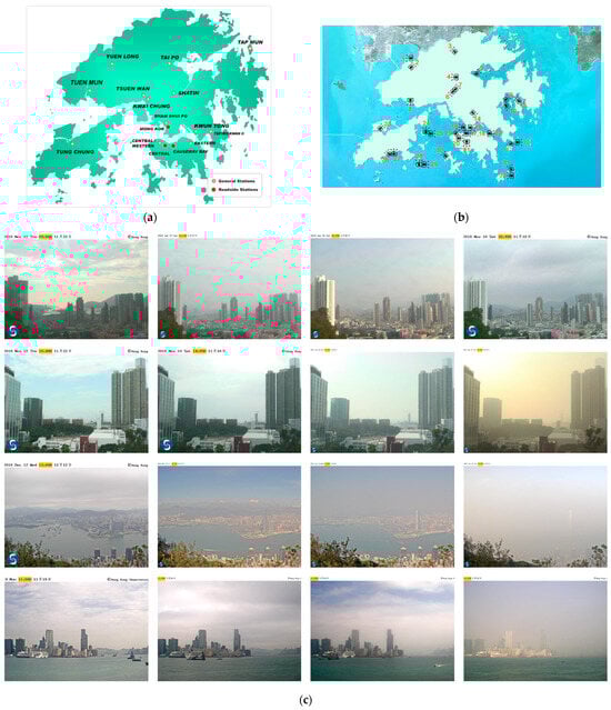
Figure 2.
(a) Location of the monitoring stations in Hong Kong (www.hko.gov.hk accessed on 11 November 2024). (b) Location of the weather cameras in Hong Kong (www.hko.gov.hk accessed on 11 November 2024). (c) Sample input images (www.hko.gov.hk accessed on 1 November 2023).
The Hong Kong Observatory’s surveillance cameras capture images every five minutes for weather monitoring purposes, providing a comprehensive data source for this algorithm. Over 300,000 images were collected through image scraping between November 2018 and early March 2019 from 14 cameras. The cameras’ locations are 1–5, 8–12, 14, 15, 17, and 19–22 in Figure 2b, which illustrates the weather cameras in Hong Kong. All cameras used for capturing these images were placed in open areas with a resolution of 1280 × 720. Samples of four of the stations utilised in the study are shown below (Figure 2c). The distance of information captured by these cameras depended on the day’s visibility. The primary purpose of these cameras was to capture weather-related information for the general public. Hong Kong data were chosen for this study because the stations and the cameras are scattered evenly, with a similar number of stations and cameras around. Also, the camera’s resolution is relatively high, which provides a good source of data for training and testing, with a setting that allows all cameras to have a long focal point, i.e., designed to the image from a far distance, which is a very good setup for the CORD model.
Meteorological data are sourced from the Climatological Information Services section of the Hong Kong Observatory’s website. This information encompasses a range of daily metrics, including mean pressure, maximum and minimum air temperatures, dew point, relative humidity, cloud cover, and total rainfall. The observatory’s webpage updates these data points daily.
Figure 2a,b illustrate that the monitoring and weather stations are well distributed across various suburbs in Hong Kong. This extensive coverage ensures a comprehensive and even distribution throughout the city, facilitating accurate estimations with the COLD framework. While COLD can be applied in any urban environment, obtaining reliable results requires data sources, such as monitoring stations and cameras, strategically placed across multiple locations to encompass the entire area. Hong Kong possesses these characteristics, making it an ideal representation for this study.
4.3. Data Preparation
The Environment Protection Department’s (EPD) air quality monitor station collects air quality data for Hong Kong. However, some data may not have been properly collected or missing. The EPD will estimate and mark the missing data with an asterisk in such cases. The collected data are also cleaned, and outliers are removed. If the data cannot be estimated, it will be marked as Not Available (N/A). Any N/A data will be replaced with zero during the data cleaning, and the asterisk will be removed for further data processing. Similarly, data collected from the Hong Kong Observatory (HKO) undergoes a similar cleaning process, including removing outliers.
4.4. Output Data Preparation
CORD was trained to predict a 24 h AQHI value using a time series with various window widths (i.e., the number of previous time steps) to predict future AQHI values. The following equation would forecast the output for the predicted value of Y at t0.
Yt0 = F(Xt−1, Xt−2 … Xt−n+1, Xt−n)
Y (t = 0) was the estimated value of time = 0, and the algorithm was trained on X (t = n) to X t = 0 if the window width was n hr. For example, if the window width is 10, the predicted value is based on the value of training data from Xt−1 to Xt−n. The first n hours of the input and output training data set were discarded.
4.5. Performance Measures
The parameter selection and performance evaluation were based on mean absolute error (MAE) and root mean square error (RMSE) measurements. These metrics are commonly employed to account for significant errors. The accuracy of the algorithms is compared based on the metrics calculated and compared for each one. RMSE is derived from the average squared difference between forecast and actual values, while MAE represents the mean difference between predicted and actual values. These metrics are calculated using the following formulas [32]:
This study employs mean absolute error (MAE), which calculates the average of the absolute differences between predicted and actual values. By assigning equal weight to all errors, regardless of their size, MAE offers valuable insights into the significance of larger errors.
Root mean square error (RMSE) is utilised in this study as well. RMSE assesses the square root of the average of the squared differences between predicted and actual values. By squaring the errors before summing, larger errors are given more weight, making RMSE particularly advantageous when large deviations are especially undesirable. Furthermore, RMSE retains the same units as the input data, enhancing its interpretability.
These matrices are commonly employed to account for significant errors. The lower the MAE and RMSE, the better a model’s predictive accuracy. Conversely, higher values of both metrics indicate a greater discrepancy between predicted and actual outcomes.
4.6. Training
CORD is built on Keras (version 2.11.0), a high-level neural network Application Programming Interface (API) written in Python 3. This open-source neural network library is designed to provide fast experimentation with deep neural networks. The data were ordered in chronological order when uploaded. The total number of records would then be counted. The scaled data were then split into a training set and a testing set; the training set contains the first 80% of the data, and the testing set contains the remaining 20% of the data, which are reserved for testing purposes and are not included in the training.
5. Evaluation and Discussion
5.1. Analysis of Results
CORD performance was tested by comparing 24 h predictions with the corresponding actual value. Three stations (Central, Eastern and Kwun Tong) were selected for the test, and the training with images and structured data was successful. The data set discussed inserted into the algorithm mentioned above also generated the outcome successfully.
A confusion matrix collects and summarises a 24 h prediction of each station. Figure 3 shows the confusion matrix for the prediction accuracy for the three stations. Figure 3a displays the confusion matrix of the predicted and actual values, while Figure 3b, shows the standardised confusion matrix for the same data set. Horizontal values represent the predicted values generated from CORD, whereas the verticals illustrate the actual values of the samples. When the predicted value matches the actual value in a confusion matrix, it falls on the diagonal. This means that the predictions are accurate and match the actual values. The values on the diagonal represent the number of correct predictions. There are 4 outcomes at AQHI level 3, 41 outcomes at AQHI level 4 and 16 outcomes at AQHI level 5 correctly predicted, while the off-diagonal values indicate the number of incorrect predictions. For example, five predictions of actual AQHI level 5 are incorrectly predicted as level 4. On-diagonal values in Figure 3b suggest the proportion of accurate predictions. AQHI level 3 has an accuracy of 100%, AQHI level 4 has an accuracy of 87% and AQHI level 5 has an accuracy of 76%. Figure 4 Compares of the actual value and the prediction by stations and Figure 5 illustrates the error vs. time by station.
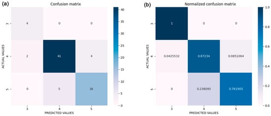
Figure 3.
(a) Confusion matrix for prediction accuracy. (b) Normalised confusion matrix for prediction accuracy.
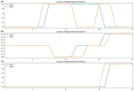
Figure 4.
Comparison of the actual value and the prediction by stations.

Figure 5.
Error vs. time by station.
5.2. Comparison of Different Models
CORD (algorithm a) performance was compared to other forecasting models using the same data set by comparing 24 h predictions against an LSTM with two hidden layers (algorithm b), a GRU with two hidden layers (algorithm c) and an ANN with two hidden layers (algorithm d). All these algorithms were built with the Keras library using Relu activation functions. All algorithms have the same number of neurons in the hidden and output layers. The inputs included all the parameters from the metrological data and the air pollution, and all models were allowed to train for the same epochs, 20 in this case. The outcome was generated successfully with the same data set inserted into the abovementioned algorithms. The 24 h prediction of each algorithm is plotted against time, as illustrated in Figure 6, Figure 7 and Figure 8. The MAE and RMSE for a 24 h prediction of the above experiment have been calculated. For a 24 h prediction, the CORD system’s mean absolute error (MAE) ranges from 0.0417 to 0.2917, and the root mean square error (RMSE) ranges from 0.0417 to 0.5401. With the same meteorological and air pollution data set, LSTM with two hidden layers has MAE ranges from 0.0833 to 0.3750 and an RMSE of 0.2287 to 0.6120 for a 24 h prediction. For GRU with two hidden layers, the MAE and RMSE range from 0.0417 to 0.25 and 0.2041 to 0.5 for a 24 h prediction. An ANN with two hidden layers has an MAE range from 0.2083 to 0.6250 and an RMSE of 0.4564 to 0.7906 for a 24 h prediction. A summary of the above outcome for each algorithm is listed in the table (Table 1) above. CORD has a similar outcome as GRU, and it has a slightly smaller error than LSTM, suggesting that CORD has a slightly better prediction capability in this test. Compared to ANN, CORD has a much smaller error, which suggests that CORD has a better prediction than ANN in this study.
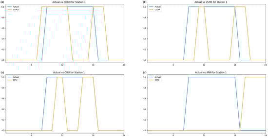
Figure 6.
Comparison of different algorithms for station 1.
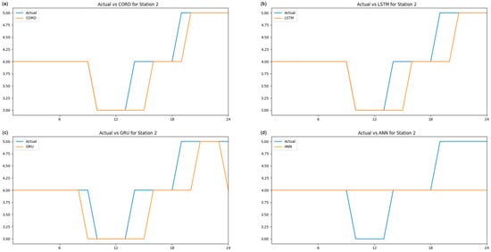
Figure 7.
Comparison of different algorithms for station 2.
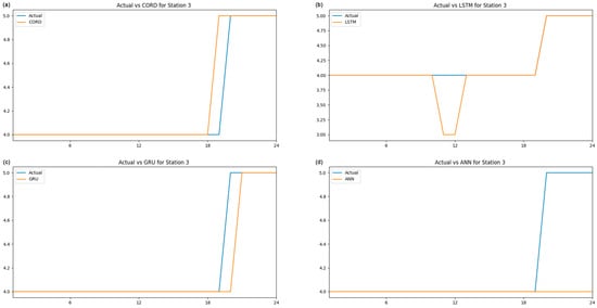
Figure 8.
Comparison of different algorithms for station 3.

Table 1.
Comparison of MAC and RMSE between different algorithms for all stations.
The coefficient of determination, denoted as R2, is conventionally utilised to evaluate the proportion of variance explained by a model in the context of continuous outcomes. A comprehensive summary of the R² values associated with each algorithm has been meticulously compiled and is presented in the table (Table 2) above. At Station 1, the R² values for all models are markedly inferior in comparison to those at other stations. For example, the CORD model demonstrates an R2 of 0.15, the LSTM model displays an R² of 0.04, and the GRU model indicates an R2 of 0.37. These low R2 values suggest that the models account for only a minor fraction of the data variance at Station 1. However, this observation does not necessarily imply inadequate model performance, as the rounding of data results in discrete values that attenuate the variability of the target variable, thereby rendering R2 less relevant as a performance metric. In contrast, at Stations 2 and 3, significantly higher R2 values are apparent for the majority of models, particularly for CORD, which records R2 values of 0.77 and 0.79, respectively. Considering that the target data are rounded, the relationship between predicted and actual values is overly simplistic, potentially inflating the R2 values and engendering a misleading interpretation of model efficacy. Furthermore, the ANN model produces “Infinity” values for R2 at Stations 2 and 3. This phenomenon occurs when the total variance of the rounded target data (the denominator in the R2 calculation) is either zero or exceedingly minimal, resulting in division by zero. This observation highlights the shortcomings of R2 for datasets characterised by rounding, as it fails to provide a meaningful evaluation of model performance.
Table 2.
Comparison of R2 between different algorithms for all stations.
R2 is intended to gauge how effectively a regression model elucidates the variance in a continuous target variable. When the target variable undergoes rounding or discretisation, the resultant rounding diminishes its variability as numerous continuous values converge into a singular rounded value. Rounding introduces discontinuities within the data, fostering a step-like relationship between predicted and actual values. This, in turn, contravenes the assumptions underpinning R2, which presumes a linear relationship between variables. As evidenced by the ANN model at Stations 2 and 3, R2 may yield “Infinity” values when the total variance associated with the rounded target data is zero or nearly negligible. This circumstance arises because R2 depends on the variance of the observed values to compute the proportion of variance explicated by the model. When the variance is minimal, the denominator of the R2 formula approaches zero, resulting in invalid outcomes.
To summarise, when predicting time series data, CORD performs slightly better than LSTM and GRU in terms of mean absolute error and root mean square error. CORD has a lower MAE and RMSE than a simple ANN algorithm, achieving greater prediction accuracy. The architecture of CORD is unique in that it combines elements of both CNN and LSTM models. Specifically, the CNN layers in CORD are used to categorise images into data that LSTM can analyse. These CNN layers can also serve as an additional data source when there are gaps in the monitoring data. By incorporating image data, CORD can achieve a slight improvement in accuracy. In this study, the LSTM layers in CORD provided good predictions. Combined with CNN, these layers could incorporate additional data from other sources, leading to an even better prediction due to the extra information. However, even without CNN, the LSTM predicted the AQHI better than ANN. This could be the reason why CORD outperformed ANN. This study is one of the first to integrate two deep learning techniques in predicting air quality using time series analytics. The scale-dependent properties of MAE and RMSE indicate that the results from this study can only be compared using metrics that are on the same scale. Furthermore, the distinctive nature of AQHI complicates comparisons with experiments conducted at different scales. A meaningful comparison can be achieved when CORD is utilised in other locations that share a common scale. This study showed that using extra images improved accuracy compared to other deep learning algorithms. CORD could be applied to other regions, but the model must be retrained. If comparison is needed, the scale of the Air Quality Index has to be aligned to perform the comparison if MAE and RMSE are used. This promising output could be applied to other air pollution measuring approaches, such as AQI.
There are a few improvements that can be made to the algorithms.
Since CORD is an LSTM-based model, it occasionally faces challenges in capturing hidden input features within long-range data sequences. This limitation arises mainly because it processes information in a single forward direction, relying solely on past data. To enhance CORD, incorporating a Bi-LSTM architecture could prove advantageous. The Bi-LSTM structure features two layers of LSTM: one that processes data in the forward direction and another that functions in reverse. This dual-layer approach enables the model to leverage both preceding and succeeding information. As a result, the Bi-LSTM model is better positioned to capture a wider array of input features, utilising data from future time steps through the backward layer. The bidirectional nature of Bi-LSTM fosters a more comprehensive and accurate representation of the input data. By considering both past and future information, the model can more effectively identify patterns, context, and dependencies within the sequence, ultimately leading to more precise predictions [19].
Although CORD works well in prediction, there is a good chance that the latest advancements, such as attention mechanisms and transformers, outperform CORD due to their ability to model intricate relationships and long-range dependencies in data. Compared to transformers, CORD is less computationally demanding. However, CORD would have the same limitations as LSTM. The first limitation is struggling to retain information over long sequences, as their memory cells can lose context. This limitation makes them less effective than transformers, which leverage self-attention to model long-term dependencies [33]. CORD also process input data sequentially, like LSTM, which is computationally inefficient for long sequences. Transformers, in contrast, use parallel processing, which improves training speed [34].
The current practice of addressing missing values in a data set typically involves replacing them with zeros. However, this approach can considerably alter the data distribution and adversely impact the training process of neural network models. Filling missing values with zeros may introduce noise, bias, and distortions within the data. Techniques like feature scaling have already been applied to reduce these effects. Nonetheless, future research on this topic should consider exploring alternative imputation methods, such as mean or median imputation, k-nearest neighbours (KNNs), or model-based techniques [35].
Addressing the time lag between actual and predicted values can enhance the performance of a recurrent neural network (RNN) model. One effective approach is to utilise the Autocorrelation Function (ACF) (https://www.geeksforgeeks.org/what-is-lag-in-time-series-forecasting/, accessed on 8 March 2025), which measures the correlation between an observation and its lagged values. The ACF plot illustrates the strength of correlation across various lags. If the time series exhibits strong correlations at specific lags, those lags can be incorporated into the model. This approach enables the model to concentrate on discerning the true underlying patterns in the data rather than merely compensating for the lag.
6. Conclusions and Recommendations
This paper presents a novel approach to predicting air quality by integrating well-structured meteorological and unstructured air pollution data with camera images. An algorithm that can perform time series-related predictions using two deep learning techniques and time series analytics has been discussed. The novelty of this study lies in its innovative integration of unstructured visual data from meteorological cameras with structured air pollution and weather data for air quality prediction. Unlike traditional models that rely solely on numerical or structured inputs, the CORD model combines image-based data with time series analytics, providing a unique approach to air quality forecasting. This dual-input framework expands the potential of deep learning applications by enabling the use of alternative data sources, such as images, to enhance prediction accuracy.
The approach utilised two types of neural networks—a convolutional neural network and a recurrent neural network with LSTM—which were trained on time series air pollutants and weather data from an air monitoring station along with over 18,000 images from the observatory weather cameras in Hong Kong. The algorithm predicts a 24 h Air Quality Health Index, a unique set of air pollution measuring systems used only in Hong Kong. The CORD algorithm has a mean absolute error of 0.2917 and a root mean square error of 0.5401, with a similar result as GRU and a slightly smaller error than LSTM. Additionally, CORD has shown better accuracy than the ANN algorithm.
While the model shows promise in predicting air quality, its limitations must be critically assessed. One of the most significant limitations of the CORD model is its dependence on the quality and availability of data. The model utilises structured data from air quality monitoring stations and unstructured data from meteorological cameras. However, the quality of these data can be inconsistent. For instance, images captured by the cameras may be affected by environmental factors such as fog, rain or snow. This can obscure visibility and result in inaccurate interpretations of air quality. Additionally, monitoring stations may experience technical malfunctions or maintenance issues, leading to missing or erroneous data. The presence of such inconsistencies can significantly impact the model’s predictive performance.
The handling of missing values is another critical issue for the CORD model. The current practice of replacing missing data with zeros can distort the underlying data distribution, introducing noise and bias into the training process. This approach may lead to misleading predictions, particularly in scenarios where the missing data point is critical for understanding air quality dynamics. Alternative imputation techniques could be explored to improve data integrity, such as mean or median imputation, k-nearest neighbours (KNNs), or model-based methods. However, the challenge remains in selecting the most appropriate imputation method that accurately reflects the underlying data characteristics. However, selecting the most appropriate imputation method remains a challenge, particularly when dealing with diverse data sources.
In terms of algorithms, the CORD model currently does not incorporate attention mechanisms, which have been shown to enhance the performance of deep learning models in various applications. Attention mechanisms allow the model to focus on specific parts of the input data that are more relevant for making predictions. By integrating attention mechanisms, the CORD model could improve its ability to identify critical features within the data, leading to more accurate air quality predictions. This integration could also help mitigate the impact of noisy or irrelevant data points on overall prediction accuracy.
It is advised that the techniques for image collection and null data handling be improved to enhance the CORD model and overcome its limitations. As the data are sourced by scraping from the Hong Kong Observatory Website, there may be occasions when the web crawler fails to gather information. Machine learning can estimate the missing data in such instances, potentially enhancing the CORD algorithm. Incorporating attention mechanisms to improve the model’s ability to capture long-term dependencies and focus on critical features within the data could further refine the model architecture. This can result in incomplete or missing data, further affecting the model’s performance. Machine learning-based techniques to estimate missing data in such scenarios could potentially mitigate this issue and improve the robustness of the model
In summary, the CORD model’s novelty lies in its ability to combine structured and unstructured data for air quality prediction, providing a unique and scalable approach to address the limitations of traditional prediction models. By implementing the proposed improvements—enhanced data handling techniques, advanced imputation methods, and attention mechanisms—the CORD model can evolve into a more robust and versatile tool for air quality prediction, ultimately contributing to better public health and environmental sustainability. Improvements in data handling techniques, such as advanced imputation methods, and the incorporation of attention mechanisms, could significantly enhance the model’s accuracy and reliability. Addressing the challenges related to data quality, availability, and collection processes will further help to develop the CORD model into a robust and versatile tool for air quality prediction. These enhancements will ensure that the model can contribute meaningfully to public health and environmental sustainability in diverse and real-world settings.
Author Contributions
Writing—original draft, K.C.; Writing—review & editing, P.M. and K.M. All authors have read and agreed to the published version of the manuscript.
Funding
This work has been partially funded by the University of the West of England (UWE), Bristol, UK, under their international collaboration program.
Data Availability Statement
The data presented in this study are available in The Hong Kong Observatory Data at https://www.hko.gov.hk/en/cis/dailyExtract.htm?y=2018&m=11, accessed on 8 March 2025. https://www.hko.gov.hk/en/wxinfo/uvinfo/dailymeanmaxuva.html, accessed on 8 March 2025. The Environment Protection Department Data at https://cd.epic.epd.gov.hk/EPICDI/air/station/, accessed on 8 March 2025. The Hong Kong Observatory Surveillance cameras picture at https://www.hko.gov.hk/en/wxinfo/ts/index_webcam.htm, accessed on 8 March 2024.
Conflicts of Interest
The authors have no relevant financial or non-financial interests to disclose. The authors have no conflicts of interest to declare that they are relevant to the content of this article. All authors certify that they have no affiliations with or involvement in any organisation or entity with any financial or non-financial interest in the subject matter or materials discussed in this manuscript. The authors have no financial/economic or proprietary interests in any material discussed in this article.
References
- Julfikar, S.K.; Ahamed, S.; Rehena, Z. Air Quality Prediction Using Regression Models. Lect. Notes Electr. Eng. 2021, 778, 251–262. [Google Scholar] [CrossRef]
- Madan, T.; Sagar, S.; Virmani, D. Air Quality Prediction using Machine Learning Algorithms-A Review. In Proceedings of the 2020 2nd International Conference on Advances in Computing, Communication Control and Networking (ICACCCN), Greater Noida, India, 18–19 December 2020; pp. 140–145. [Google Scholar] [CrossRef]
- Sahoo, L.; Praharaj, B.B.; Sahoo, M.K. Air Quality Prediction Using Artificial Neural Network. Adv. Intell. Syst. Comput. 2021, 1248, 31–37. [Google Scholar] [CrossRef]
- Li, X.; Peng, L.; Yao, X.; Cui, S.; Hu, Y.; You, C.; Chi, T. Long short-term memory neural network for air pollutant concentration predictions: Method development and evaluation. Environ. Pollut. 2017, 231, 997–1004. [Google Scholar] [CrossRef]
- Umar, I.K.; Nourani, V.; Gökçekuş, H. A novel multi-model data-driven ensemble approach for the prediction of particulate matter concentration. Environ. Sci. Pollut. Res. 2021, 28, 49663–49677. [Google Scholar] [CrossRef] [PubMed]
- Kök, I.; Şimşek, M.U.; Özdemir, S. A deep learning model for air quality prediction in smart cities. In Proceedings of the 2017 IEEE International Conference on Big Data (Big Data), Boston, MA, USA, 11–14 December 2017; pp. 1983–1990. [Google Scholar] [CrossRef]
- Chan, K.; Matthews, P.; Munir, K. A Framework for the Estimation of Air Quality by Applying Meteorological Images: Colours-of-the-Wind (COLD). Environments 2023, 10, 218. [Google Scholar] [CrossRef]
- Gardner, M.W.; Dorling, S.R. Artificial Neural Networks (The Multilayer Perceptron)–A Review Of Applications In The Atmospheric Sciences. Atmos. Environ. 1998, 32, 2627–2636. [Google Scholar] [CrossRef]
- Bengio, Y. Practical Recommendations for Gradient-Based Training of Deep Architectures; Springer: Berlin/Heidelberg, Germany, 2012. [Google Scholar]
- Biancofiore, F.; Verdecchia, M.; Di Carlo, P.; Tomassetti, B.; Aruffo, E.; Busilacchio, M.; Bianco, S.; Di Tommaso, S.; Colangeli, C. Analysis of surface ozone using a recurrent neural network. Sci. Total Environ. 2015, 514, 379–387. [Google Scholar] [CrossRef] [PubMed]
- Biancofiore, F.; Busilacchio, M.; Verdecchia, M.; Tomassetti, B.; Aruffo, E.; Bianco, S.; Di Tommaso, S.; Colangeli, C.; Rosatelli, G.; Di Carlo, P. Recursive neural network model for analysis and forecast of PM10 and PM2.5. Atmos. Pollut. Res. 2017, 8, 652–659. [Google Scholar] [CrossRef]
- Comrie, A.C. Comparing Neural Networks and Regression Models for Ozone Forecasting. J. Air Waste Manag. Assoc. 1997, 47, 653–663. [Google Scholar] [CrossRef]
- Elman, J.L. Finding Structure in Time. Cogn. Sci. 1990, 14, 179–211. [Google Scholar] [CrossRef]
- Elangasinghe, M.A.; Singhal, N.; Dirks, K.N.; Salmond, J.A.; Samarasinghe, S. Complex time series analysis of PM10 and PM2.5 for a coastal site using artificial neural network modelling and k-means clustering. Atmos. Environ. 2014, 94, 106–116. [Google Scholar] [CrossRef]
- Che, Z.; Purushotham, S.; Cho, K.; Sontag, D.; Liu, Y. Recurrent Neural Networks for Multivariate Time Series with Missing Values. Sci. Rep. 2018, 8, 6085. [Google Scholar] [CrossRef] [PubMed]
- Graves, A. Generating Sequences With Recurrent Neural Networks. arXiv 2013, arXiv:1308.0850. [Google Scholar]
- Koehrsen, W. Recurrent Neural Networks by Example in Python. Available online: https://towardsdatascience.com/recurrent-neural-networks-by-example-in-python-ffd204f99470 (accessed on 8 March 2025).
- Zhou, X.; Xu, J.; Zeng, P.; Meng, X. Air Pollutant Concentration Prediction Based on GRU Method. In Proceedings of the Journal of Physics: Conference Series; Institute of Physics Publishing: Bristol, UK, 2019; Volume 1168. [Google Scholar]
- Vankadara, R.K.; Mosses, M.; Siddiqui, M.I.H.; Ansari, K.; Panda, S.K. Ionospheric Total Electron Content Forecasting at a Low-Latitude Indian Location Using a Bi-Long Short-Term Memory Deep Learning Approach. IEEE Trans. Plasma Sci. 2023, 51, 3373–3383. [Google Scholar] [CrossRef]
- Reddybattula, K.D.; Nelapudi, L.S.; Moses, M.; Devanaboyina, V.R.; Ali, M.A.; Jamjareegulgarn, P.; Panda, S.K. Ionospheric TEC Forecasting over an Indian Low Latitude Location Using Long Short-Term Memory (LSTM) Deep Learning Network. Universe 2022, 8, 562. [Google Scholar] [CrossRef]
- Zhang, R.; Li, H.; Shen, Y.; Yang, J.; Li, W.; Zhao, D. Deep Learning Applications in Ionospheric Modeling: Progress, Challenges, and Opportunities. Remote Sens. 2025, 17, 124. [Google Scholar] [CrossRef]
- Freeman, B.S.; Taylor, G.; Gharabaghi, B.; Thé, J. Forecasting air quality time series using deep learning. J. Air Waste Manag. Assoc. 2018, 68, 866–886. [Google Scholar] [CrossRef]
- Gómez, P.; Nebot, A.; Ribeiro, S.; Alquézar, R.; Mugica, F.; Wotawa, F. Local maximum ozone concentration prediction using soft computing methodologies. Syst. Anal. Model. Simul. 2003, 43, 1011–1031. [Google Scholar] [CrossRef]
- O’Shea, K.; Nash, R. An Introduction to Convolutional Neural Networks. arXiv 2015, arXiv:1511.08458. [Google Scholar]
- Bezdan, T.; Bačanin Džakula, N. Convolutional Neural Network Layers and Architectures; Singidunum University: Beograd, Serbia, 2019; pp. 445–451. [Google Scholar]
- Saleem, M.A.; Senan, N.; Wahid, F.; Aamir, M.; Samad, A.; Khan, M. Comparative Analysis of Recent Architecture of Convolutional Neural Network. Math. Probl. Eng. 2022, 2022, 7313612. [Google Scholar] [CrossRef]
- Taye, M.M. Theoretical Understanding of Convolutional Neural Network: Concepts, Architectures, Applications, Future Directions. Computation 2023, 11, 52. [Google Scholar] [CrossRef]
- Bayat, O.; Aljawarneh, S.; Carlak, H.F. International Association of Researchers, Institute of Electrical and Electronics Engineers, and Akdeniz Universitesi. In Proceedings of the 2017 International Conference on Engineering & Technology (ICET’2017): Akdeniz University, Antalya, Turkey, 21–23 August 2017; ISBN 9781538619490. [Google Scholar]
- Indolia, S.; Goswami, A.K.; Mishra, S.P.; Asopa, P. Conceptual Understanding of Convolutional Neural Network—A Deep Learning Approach. Procedia Comput. Sci. 2018, 132, 679–688. [Google Scholar] [CrossRef]
- Environmental Protection Department Hong Kong (HKEPD). Annual Air Quality Monitoring Report; Marlborough District Council: Blenheim, New Zealand, 2022.
- Chan, C.K.; Yao, X. Air pollution in mega cities in China. Atmos. Environ. 2008, 42, 1–42. [Google Scholar] [CrossRef]
- Hasnain, A.; Sheng, Y.; Hashmi, M.Z.; Bhatti, U.A.; Hussain, A.; Hameed, M.; Marjan, S.; Bazai, S.U.; Hossain, M.A.; Sahabuddin, M.; et al. Time Series Analysis and Forecasting of Air Pollutants Based on Prophet Forecasting Model in Jiangsu Province, China. Front. Environ. Sci. 2022, 10, 945628. [Google Scholar] [CrossRef]
- Vaswani, A.; Shazeer, N.; Parmar, N.; Uszkoreit, J.; Jones, L.; Gomez, A.N.; Kaiser, Ł.; Polosukhin, I. Attention is all you need. In Proceedings of the 31st Conference on Neural Information Processing Systems (NIPS 2017), Long Beach, CA, USA, 4–9 December 2017; pp. 5999–6009. [Google Scholar]
- Brown, T.B.; Mann, B.; Ryder, N.; Subbiah, M.; Kaplan, J.; Dhariwal, P.; Neelakantan, A.; Shyam, P.; Sastry, G.; Askell, A.; et al. Language Models are Few-Shot Learners. Adv. Neural Inf. Process. Syst. 2020, 33, 1877–1901. [Google Scholar]
- Hron, K.; Templ, M.; Filzmoser, P. Imputation of missing values for compositional data using classical and robust methods. Comput. Stat. Data Anal. 2010, 54, 3095–3107. [Google Scholar] [CrossRef]
Disclaimer/Publisher’s Note: The statements, opinions and data contained in all publications are solely those of the individual author(s) and contributor(s) and not of MDPI and/or the editor(s). MDPI and/or the editor(s) disclaim responsibility for any injury to people or property resulting from any ideas, methods, instructions or products referred to in the content. |
© 2025 by the authors. Licensee MDPI, Basel, Switzerland. This article is an open access article distributed under the terms and conditions of the Creative Commons Attribution (CC BY) license (https://creativecommons.org/licenses/by/4.0/).