Article

Significance of Cloud Microphysics and Cumulus Parameterization Schemes in Simulating an Extreme Flood-Producing Precipitation Event in the Central Himalaya

Department of Earth and Atmospheric Sciences, University of Alberta, Edmonton, AB T6G 2E3, Canada
*
Author to whom correspondence should be addressed.
Atmosphere 2025, 16(3), 298; https://doi.org/10.3390/atmos16030298
Submission received: 10 January 2025 / Revised: 25 February 2025 / Accepted: 25 February 2025 / Published: 3 March 2025
(This article belongs to the Section Atmospheric Techniques, Instruments, and Modeling)

Abstract

:
Between 11 and 14 August 2017, the southern belt of the central Himalaya experienced extreme precipitation, with some stations recording more than 500 mm of accumulated rainfall, which resulted in widespread, devastating flooding. Precipitation was concentrated over the sub-Himalaya, and the established forecasting systems failed to predict the event. In this study, we evaluate the performance of six cloud microphysics schemes in the Weather Research and Forecasting (WRF) model forced with the advanced ERA5 dataset. We also examine the importance of the cumulus scheme in WRF at 3 km horizontal grid spacing in highly convective events like this. Six WRF simulations, each with one of the six different microphysics schemes with the Kain–Fritsch cumulus scheme turned off, all fail to reproduce the spatial variability of accumulated precipitation during this devastating flood-producing precipitation event. In contrast, the simulations exhibit greatly improved performance with the cumulus scheme turned on. In this study, the cumulus scheme helps to initiate convection, after which grid-scale precipitation becomes dominant. Amongst the different simulations, the WRF simulation using the Morrison microphysics scheme with the cumulus turned on displayed the best performance, with the smallest normalized root mean square error (NRMSE) of 0.25 and percentage bias (PBIAS) of −6.99%. The analysis of cloud microphysics using the two best-performing simulations reveals that the event is strongly convective, and it is essential to keep the cumulus scheme on for such convective events and capture all the precipitation characteristics showing that in regions of extreme topography, the cumulus scheme is still necessary even down to the grid spacing of at least 3 km.

1. Introduction

An accurate weather forecast is essential to minimize the effect of extreme weather events. Modern-day weather forecasting tools involve various ground and satellite-based observations of the precipitating systems as well as numerical weather model predictions. Numerical weather models (NWMs) predict the trajectory and progression of the atmospheric variables over time, allowing effective short-range, medium-range, and long-range forecasts. A complicating factor for numerical weather prediction in this region is that large spatial variability in the weather conditions is observed due to rapidly varying topographic structures in the Himalaya [1,2,3,4]. So, the NWMs configured at a small grid spacing are crucial to making localized weather predictions [1,2]. However, the NWMs require rigorous testing and validation to find the most accurate physics configuration for reliable weather forecasting in this region [5,6,7].
In recent years, the Weather Research and Forecasting (WRF) model has been widely used over the Himalaya (e.g., Bonekamp et al. [2,8]; Collier and Immerzeel [9]; Karki et al. [1,5]; Orr et al. [6]; Tiwari and Bush [10]). The WRF model is an open-source, mesoscale atmospheric model used for numerical weather prediction and atmospheric research [11]. In Nepal, the Meteorological Forecasting Division (MFD) of the Department of Hydrology and Meteorology uses the WRF model at 4 km horizontal grid spacing to aid in weather forecasting over Nepal. In the WRF model, cloud microphysics is vital in controlling cloud particles’ formation, growth, distribution, and precipitation development. Broadly, two categories of cloud microphysics schemes are available within the WRF model: single-moment and double-moment. The single-moment microphysics schemes only predict the mass mixing ratio of the cloud and precipitation particles, while the double-moment schemes predict the mass mixing ratio and number concentration. The Lin microphysics scheme [12] used in the WRF model by the MFD is a single-moment scheme that includes ice, snow, and graupel processes.
Despite implementing several weather and flood forecasting systems, including numerical weather prediction models, across local, regional, and global levels, such prediction systems failed to predict the devastating 2017 flooding event [13]. During the second week of 2017 (11–14 August), intense precipitation falling over the sub-Himalaya (elevations up to 1200 m above mean sea level) resulted in one of the most extreme flooding disasters in the history of Nepal, affecting 35 districts along the southern parts of Nepal. In contrast to all other flooding disasters in Nepal, which are caused by the large rivers, like Koshi, Gandaki, Karnali, and their tributaries, this event was the result of a series of flash floods in the ephemeral rivers originating from the sub-Himalaya. A total accumulated precipitation of >500 mm was recorded during 11–16 August 2017 by several weather stations across Nepal (Figure 1). The satellite-based Global Precipitation Measurement (GPM) data also show a band of strong precipitation along the southern belt of Nepal (Figure 1b). According to a report produced by the Ministry of Home Affairs, Nepal [14], more than 80% of the area in the affected districts was inundated during the flooding events, and the death toll during the event was 160 with more than 70 people missing. The National Planning Commission (NPC) of Nepal estimated around 1,688,474 people were directly affected by the disaster [15].
Reliable flood forecasting requires an accurate input of precipitation data from extensively validated atmospheric models. Apart from a model’s horizontal and vertical grid spacing, the selection of model physics and the quality of the forcing datasets are equally crucial for an accurate prediction of the atmospheric variables. Thus, the main objective of this study is to evaluate six different cloud microphysics schemes in WRF to reproduce the devastating flood-producing precipitation event that caused the August 2017 disaster in Southern Nepal. We configure the WRF model with two nested domains of 15 and 3 km horizontal grid spacing. Furthermore, our initial experiments (not published) with ERA-Interim and NCEP forcings in the WRF model at 3 km without the cumulus parameterization scheme did not yield promising results. Since the grid spacing of those datasets is large (0.75°× 0.75° for ERA-Interim and 2.5° × 2.5° for NCEP), they may provide weak forcing, resulting in a significant precipitation underestimation. Additionally, the WRF model, even at a grid spacing of 3 km, may not explicitly resolve convection forced by a sub-grid-scale Himalayan topography, although the need for cumulus parameterization for grid spacing between 3 and 10 km (often defined as a grey zone) is still a topic of debate. However, some studies have proven that cumulus parameterization at this grey zone improves precipitation simulation [16,17,18,19]. So, in this study, we force the WRF model with ERA5 datasets (30 km × 30 km) and perform sensitivity experiments with cumulus parameterization both on and off at 3 km horizontal grid distance using six different cloud microphysics schemes. From this suite of sensitivity experiments, we also evaluate the cloud microphysics of two of the best-performing simulations to get insights into the nature of cloud formation during convection over steep topography. Finally, we expand geographically outward to explore the synoptic conditions surrounding this extreme flooding event to aid in predicting the possibility of such events in the future.

2. Materials and Methods

2.1. Model Description

In this study, we use the Weather Research and Forecasting (WRF) model version 4.2.1 to simulate the atmospheric conditions from 5 to 20 August 2017 using various cloud microphysics schemes. WRF is a mesoscale atmospheric model used for both weather forecasting and atmospheric research. We configure the WRF model with two nested domains of 15 km × 15 km (D1) and 3 km × 3 km (D2) horizontal grid sizes. Geographically, D1 covers much of South Asia, the Himalaya, and the Tibetan Plateau, whereas D2 covers the Nepalese Himalaya (Figure 2a,b, respectively). The top model pressure level is set to 50 hPa, with the domains configured with 50 vertical layers, 4 soil layers, and 1 surface layer. The initial condition for the model simulations is obtained from the ERA5 reanalysis dataset, which is available at its original grid size of 31 km. The model physics and dynamics packages used are presented in Table 1.
This study employed the one-way nesting approach, with D1 receiving initial conditions from the ERA5 data and D2 receiving initial conditions from D1 runs. The cumulus scheme is turned on for D1 simulations. The model simulation started on 5 August 2017 and ended on 20 August 2017. The first three days of the simulation are considered model spin-up periods and are not used for the analysis. The D2 simulations consist of the model runs with both cumulus schemes turned on and off, totaling 12 runs.
First, we ran D2 simulations with four selected microphysics and two cumulus parameterization schemes (Kain–Fritsch (KF) and Betts–Miller—Janjić (BMJ)). The KF scheme is based on mass flux schemes, as they account for entrainment, detrainment, and cloud-scale downdrafts improving the deep convection simulation [20]. Likewise, the BMJ is a relaxation-type cumulus scheme suitable for large-scale convection, as it adjusts temperature and moisture profile towards an equilibrium station [24]. In this study, we found that the simulations with the KF cumulus scheme produced better results than those with the BMJ scheme. The improvement of the precipitation accumulation using the KF scheme may be due to its improved representation of deep convection, convection triggering mechanisms that rely on convective instability, and various other cloud processes like entrainment, downdrafts, and moisture adjustment.

2.2. Description of Cloud Microphysics Schemes

In the WRF model, cloud microphysics controls the formation, growth, and distribution of cloud particles and precipitation development. Two types of microphysics schemes exist in the WRF model: single-moment schemes and double-moment schemes. The main difference between these schemes is that the single-moment schemes only predict the mass mixing ratio of the cloud and precipitation particles, whereas the double-moment schemes, in addition to this, also predict the number concentration. Thus, due to their advanced predictability, double-moment schemes are computationally more expensive than single-moment schemes but presumably provide advanced predictability by calculating and providing more information.
In this study, we test the sensitivity of six different cloud microphysics schemes in simulating the extreme precipitation event over the central Himalaya during 11–14 August 2017. Table 2 lists these microphysics schemes along with their characteristics.

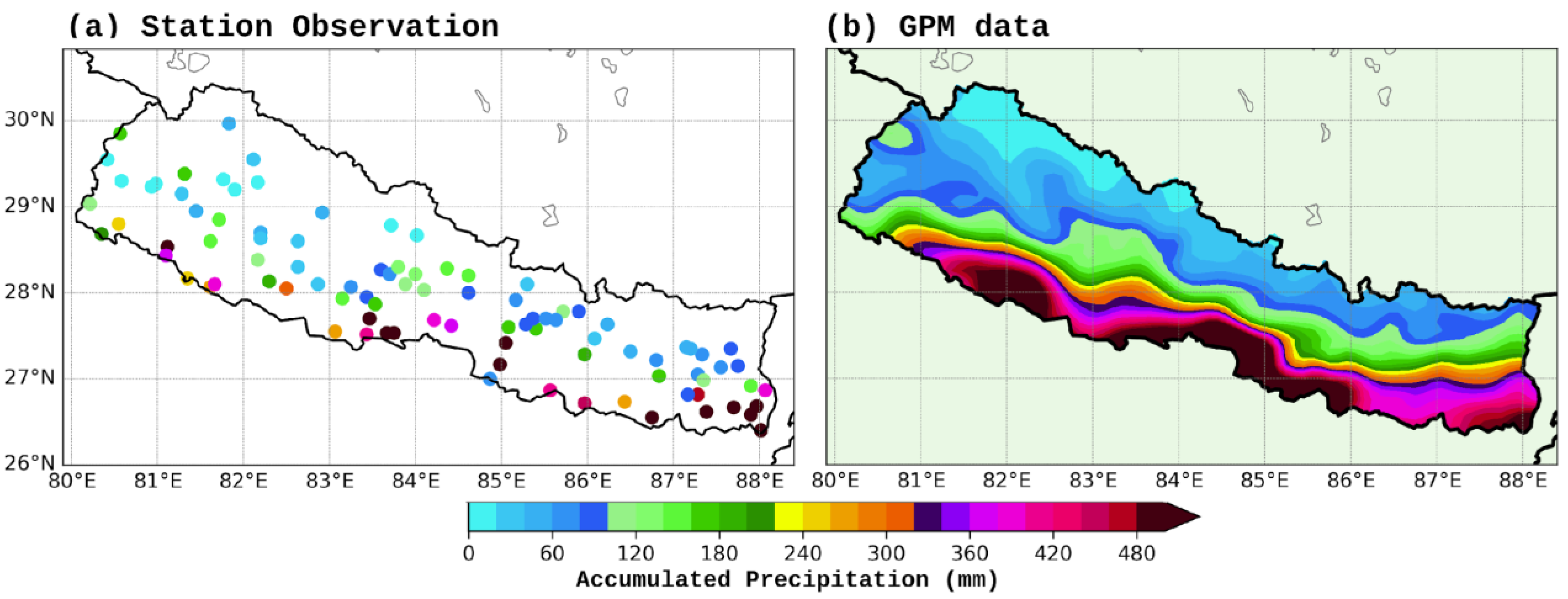
2.3. Station and Satellite Observation

We use daily accumulated precipitation recorded at 95 weather stations across Nepal (Figure 1a) and a half-hourly Global Precipitation Mission (GPM) satellite product (Figure 1b; [31]) to evaluate the performance of individual WRF simulations using different cloud microphysics schemes. The station data are available at a daily timestep and can be accessed at the Department of Hydrology and Meteorology, Nepal. Likewise, the GPM data is available at half-hourly timestep and a horizontal grid spacing of 10 km × 10 km. Studies have shown that the GPM data can reproduce the spatial and temporal features of monsoon precipitation very well [32,33].
We also use the Second Modern-ERA Retrospective analysis for Research and Applications (MERRA-2) cloud diagnostic data (Global Modeling and Assimilation Office (GMAO), 2015) to compare with selected WRF simulated hydrometeors. The MERRA-2 cloud diagnostic data contain two variables, mass fraction of cloud liquid water (QL, kg/kg) and mass fraction of cloud ice water (QI, kg/kg), which are used in cloud microphysics study. The MERRA-2 cloud diagnostic data can be accessed at https://disc.gsfc.nasa.gov/datasets/M2T3NPCLD_5.12.4/summary?keywords=cloud%20water (accessed on 21 September 2024).

2.4. Model Evaluation

We evaluate the precipitation simulated by different WRF microphysics schemes over the three altitude zones of Nepal. These three zones are defined as Z1, the Terai (Indo-Gangetic plain) and the Siwalik regions (60–1300 m amsl); Z2, the middle mountains (1300–3000 m amsl); and Z3, the high mountains (>3000 m amsl). Since the intense precipitation is concentrated over Z1 (c.f. Figure 1), we perform statistical analysis over Z1 only.
We name simulations without the cumulus scheme as “microphysics_sim” (for example, Morrison_sim) and simulations with the cumulus scheme on as “microphysics_cu_sim” (for example, Morrison_cu_sim). To evaluate the model performance, we have selected the following statistical parameters, as they provide the quantification of model errors.

2.4.1. Percentage Bias (PBIAS)

Percentage bias is a normalized metric used to evaluate the difference between the simulated precipitation and the observed precipitation. Mathematically, PBIAS is defined in Equation (1).
P B I A S = i = 1 n ( M i O i ) i = 1 n O i × 100
where, M i is the model precipitation and O i is the observed precipitation. The quantities in the numerator and denominator are spatially averaged values summed over model simulation days. Based on the value of P B I A S , we categorize the simulated precipitation as underestimation ( P B I A S < 10 % ), overestimation ( P B I A S > 10 % ), and nearly equal ( 10 % P B I A S 10 % ).
The smaller value of observed precipitation may sometimes lead to a misleading PBIAS value, so we also use other error metrics to evaluate model performance.

2.4.2. Normalized Root Mean Square Error

The RMSE is the quadratic mean of the difference between observed and simulated variables. The smaller the value of RMSE, the better the model performance. The RMSE can be calculated as
R M S E = 1 n i = 1 n M i O i 2
The NRMSE is then calculated as
N R M S E = R M S E O m a x O m i n
The lower the value of NRMSE, the smaller the difference between the observed and simulated data.

2.4.3. Coefficient of Determination (R2)

We also compute the R2 value to evaluate the linear relationships between the observations and simulations:
R 2 = 1 S S R S S T
where SSR is the sum of squared differences between observed and simulated values and SST is the total sum of squared differences between observed values and their mean. We use the Python 3.1 library scikit-learn to compute R2.

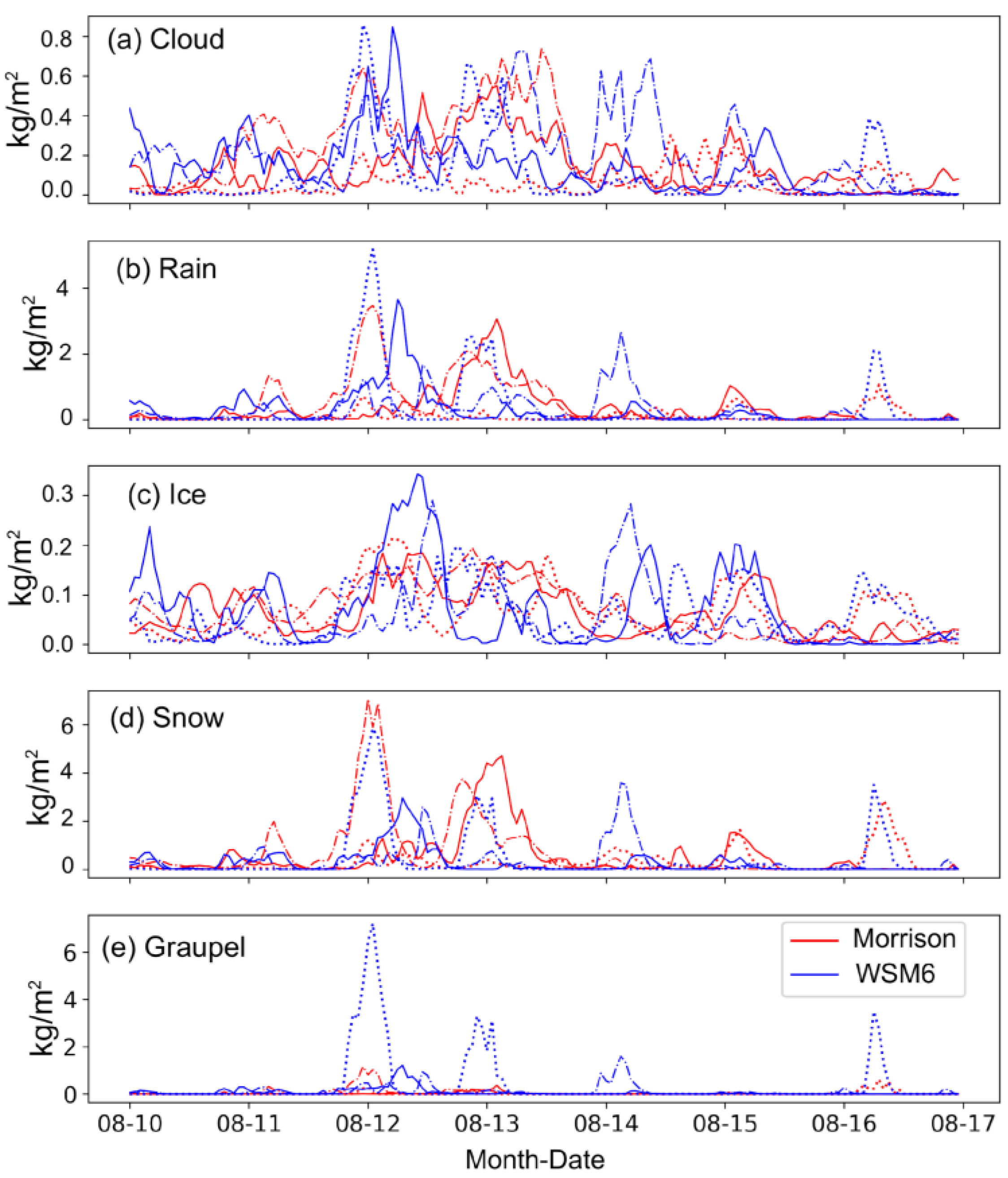
2.5. Column Density of Hydrometeors

We compute the column density of hydrometeors to examine the cloud microphysics over 11–14 August 2017. The column density of hydrometeors (CDH) is computed as
C D H = ρ ( z ) q ( z ) d z
where ρ is air density (kg/m3), q is the hydrometeor mixing ratio (kg/kg), and d z is the thickness of the atmospheric layer (m).

3. Results

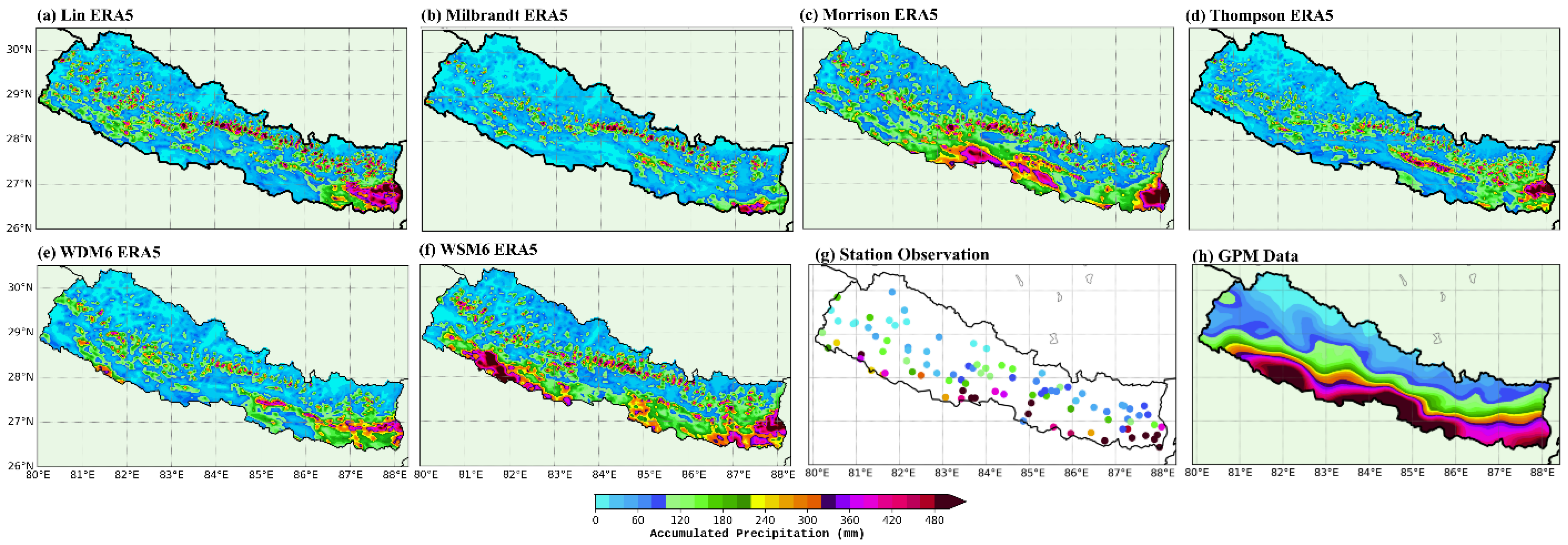
3.1. Simulations with Cumulus Parameterization off

The WRF simulations for D2 with cumulus parameterization turned off all fail to reproduce the precipitation accumulation during 11–16 August 2017 over southern Nepal, to varying degrees (Figure 3). Amongst the six simulations, the WSM6_sim displays the best spatial pattern, including substantial precipitation accumulations over south-western and south-eastern Nepal, but it nevertheless fails to capture the significant precipitation intensity over south-central Nepal. Likewise, the Morrison_sim shows precipitation accumulation over south-central and south-eastern Nepal but does not reproduce precipitation accumulation over south-western Nepal. This suggests that even with the improved forcing of ERA5, WRF simulations with various microphysics schemes fail to capture the flood-producing precipitation over the sub-Himalaya and the Indo-Gangetic plains of Nepal.

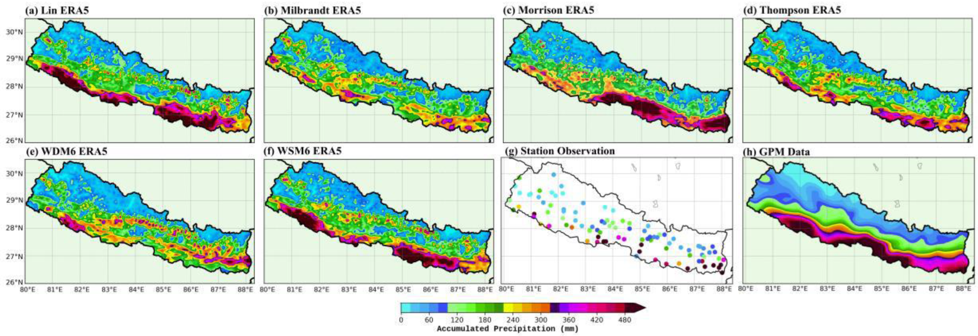
3.2. Simulations with Cumulus Parameterization Turned on

With the cumulus parameterization turned on in the D2 simulations, a significant improvement is noted in the spatial distribution of accumulated precipitation, which becomes comparable with the station and satellite observations for many of the simulations (Figure 4). All the numerical simulations produce intense rainfall along the southern belt of Nepal and most (Lin_cu_sim, Morrison_cu_sim, Thompson_cu_sim, and WSM6_cu_sim) capture the regions of extreme precipitation during the flood-producing event, although the other two (Milbrandt_cu_sim and WDM6_cu_sim) do not.
A statistical comparison of these WRF simulations with station data over Z1 reveals the smallest NRMSE for the Morrsion_cu_sim, followed by the WSM6_cu_sim. Furthermore, the values of PBIAS for both the Morrison_cu_sim and WSM6_cu_sim are less than 10%, implying a higher accuracy of the simulations (Figure 5a). The coefficient of determination ( R 2 ) for the Morrison_cu_sim is 0.74, demonstrating a strong linear relationship between the modelled and observed precipitation. On the other hand, the WDM6_cu_sim exhibits the highest NRMSE and PBIAS, displaying the poorest performance statistically (Figure 5c). The reason behind the poorest performance of WDM6_cu_sim may be due to weaker convective rainfall produced by a reduced rainwater mixing ratio because of the production of excessive cloud water [26]. Overall, the statistical parameters demonstrate that the double-moment Morrison microphysics scheme with cumulus parameterization outperforms all other model runs for the flood-producing precipitation simulation over southern Nepal.
We further evaluate the temporal evolution of precipitation by comparing the WRF simulations with the hourly GPM data over three regions, B1, B2, and B3, as shown in Figure 2b. During the monsoon season, it is typical to observe precipitation occurring throughout the day. As per the GPM data, precipitation started in the afternoon on 11 August and ended in the afternoon on 12 August (Figure 6a). During this period, three GPM precipitation peaks were observed, and the Lin_cu_sim captures the timing of these three peaks. Amongst the other simulations, there are discrepancies regarding the timing of the GPM precipitation peaks. However, the Morrison_cu_sim captures the last two peaks, with some mismatch in the timing of the peaks. Over B2, the first precipitation peak occurred on the evening of 11 August, and the second was observed in the late evening of 12 August (Figure 6b). Despite overestimating the precipitation magnitude, the Morrison_cu_sim captures both the precipitation peaks over B2. Over B3, all the simulations reproduce the GPM precipitation peaks (Figure 6c).

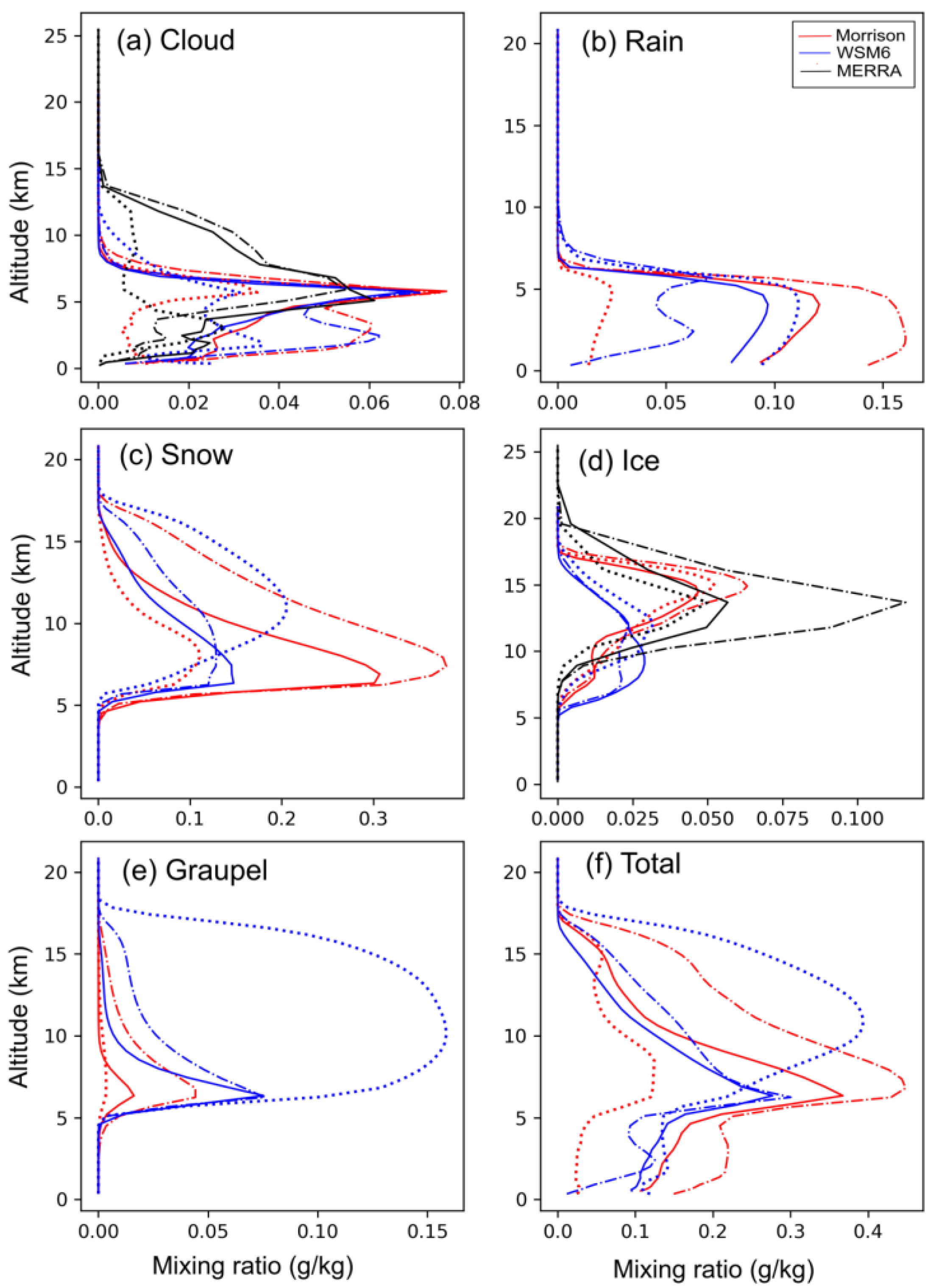
3.3. Cloud Microphysics

According to spatial distribution and our statistical analysis, we chose the two best-performing simulations (Morrison_cu_sim and WSM6_cu_sim) to investigate further the cloud microphysics over the three regions of intense precipitation indicated by the three boxes in Figure 2b (B1, B2, and B3). The column density of cloud remains high at various regions throughout the time series (Figure 7a); however, the peaks of column density of rain coincide with the timing of intense precipitation measured at the surface (Figure 7b and c.f. Figure 6). Over B1, the GPM data show three precipitation peaks between 12–13 August 2017, and the column density of cloud, rain, snow, and ice from the WSM6_cu_sim display a peak around the afternoon of 12 August, which coincides with the peak precipitation observed during that time (c.f. Figure 6a). The Morrison_cu_sim, however, produces peak column densities of hydrometeor particles around midnight to the early morning of 13 August, and the model simulates a precipitation peak around this time, consistent with the GPM precipitation peak. Furthermore, the Morrison_cu_sim captures both precipitation peaks over B2, with the column density of hydrometeors consistent with those precipitation peaks (Figure 7 and c.f. Figure 6b). On 12 August, the Morrision_cu_sim over B2 and WSM6_cu_sim over B3 simulate 6 kg/m2 column density of snow. Additionally, the WSM6_cu_sim shows >6 kg/m2 column density of graupel on 12 August.
We further investigate the vertical distribution of hydrometeor particles to gain a more detailed insight into the nature of this precipitating system. For reference, we use the MERRA-2 cloud diagnostics data on cloud liquid water and cloud ice water, which helps us understand the type of precipitation system and the distribution of liquid and frozen hydrometeors in the atmosphere. The MERRA-2 cloud data contain two variables: mass fraction of cloud ice water and mass fraction of cloud liquid water. We converted these variables to mixing ratio to plot them with the WRF variables.
The vertical distribution of spatially averaged hydrometeors, averaged over 11–14 August 2017, demonstrates a similarity in cloud droplet and ice particle distribution between the simulations and satellite measurements across all three regions. Additionally, the microphysical behaviour demonstrated by both simulations (Morrison_cu_sim and WSM6_cu_sim) indicates a highly convective storm with significant updrafts characterized by the presence of both liquid droplets and ice particles. The peak cloud mixing ratio is observed at 6 km above the surface, while the peak ice mixing ratio is observed between 10 and 15 km above the surface (Figure 8a,d).

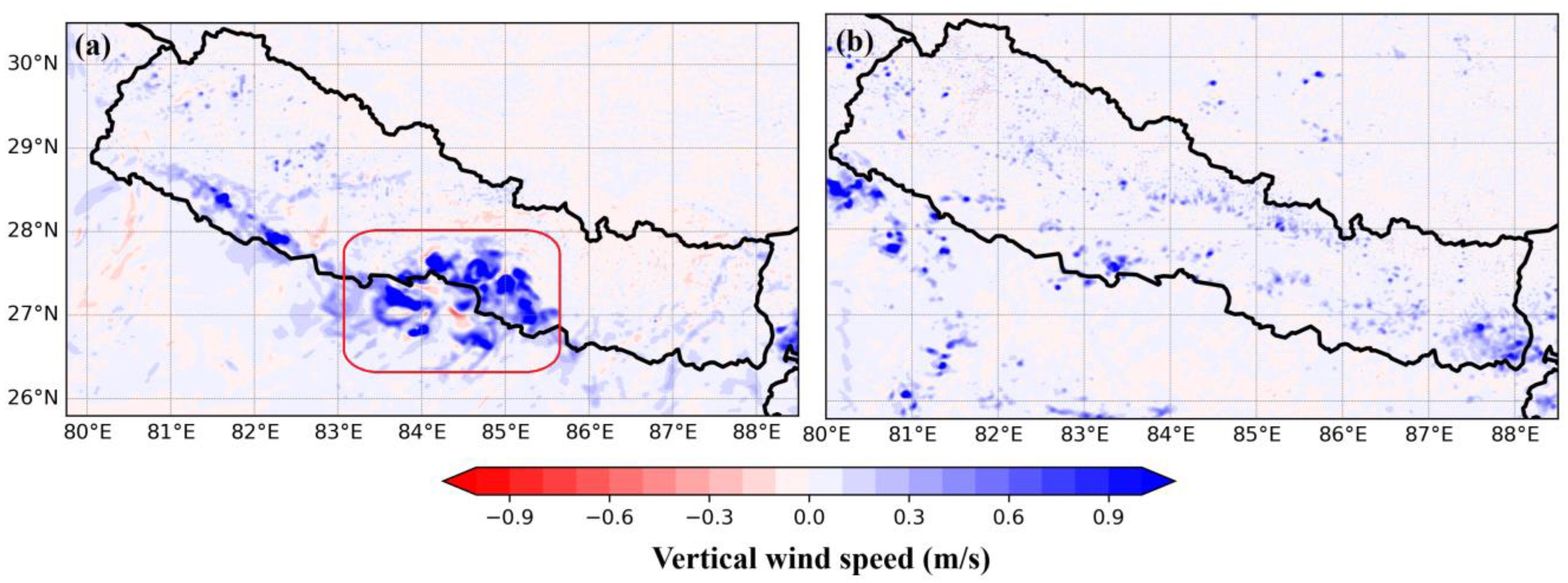
3.4. Role of Cumulus Scheme in Triggering Convection

The cumulus scheme over the complex Himalayan topography plays a crucial role in triggering an initial convection. The comparison of vertical wind speed between the Morrison_cu_sim and Morrison_sim shows that, at 3 km grid spacing, the cumulus scheme is necessary to initiate convection (Figure 9). The region of strong convection (marked by a red rectangle in Figure 9a) coincides with the area of intense precipitation shown in Figure 1. On the other hand, with the cumulus scheme turned off, the WRF model at a 3 km horizontal grid size produces small, scattered convective cells, which cannot produce intense precipitation.
We further analyzed the hourly accumulated grid-scale precipitation and the hourly accumulated cumulus precipitation produced by the Morrison_cu_sim over the three regions (B1, B2, and B3) defined in Figure 2b. The cumulus scheme initially triggers the updrafts, and once the convection is set up, the model explicitly simulates precipitation. For instance, the grid-scale precipitation peak over B2 observed around August 12 at 00:00 local time (shown in the red rectangle in Figure 10b) results from strong convection (within the red rectangle in Figure 9a) triggered by the cumulus scheme, which further justifies that at 3 km grid spacing, we still need the cumulus parameterization to trigger convection, and once the convection initiates, the model then explicitly simulates the precipitation.

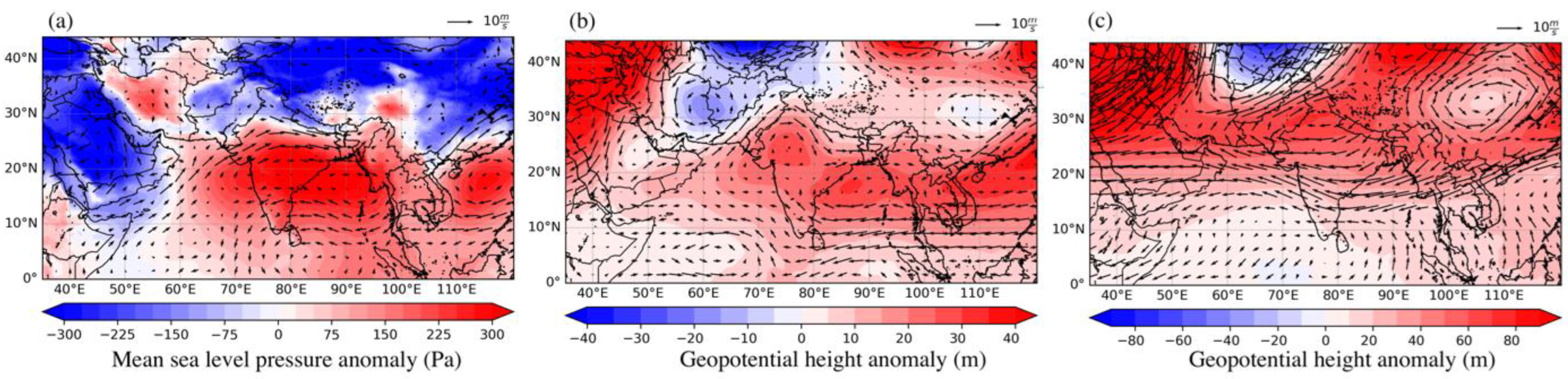
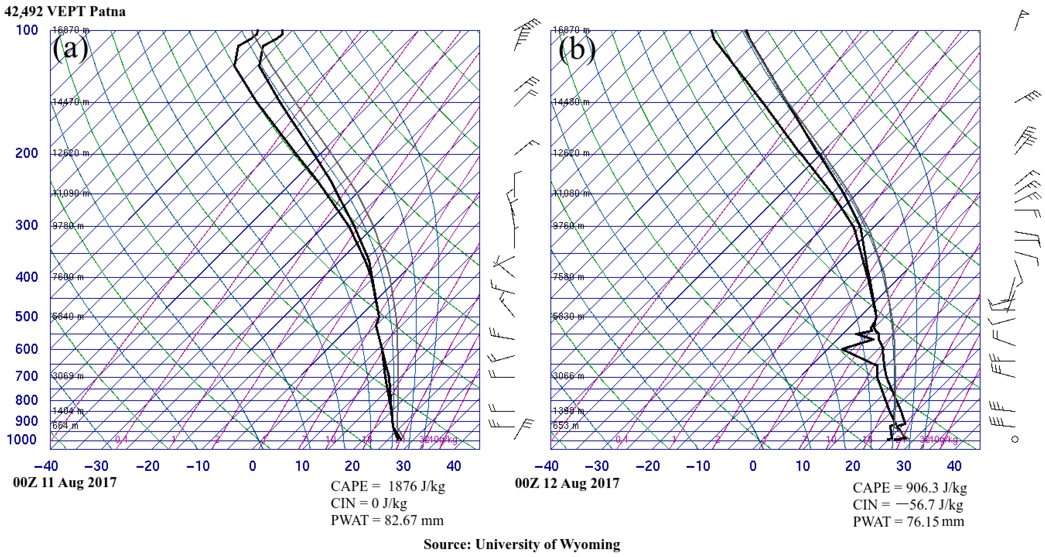
3.5. Synoptic Conditions Surrounding the Event

The synoptic conditions surrounding the event are summarized in Figure 11. The mean sea level pressure (MSLP) anomaly during this event shows an elevated MSLP over a large part of India, the Arabian Sea, the Bay of Bengal, and parts of Southeast Asia and a negative MSLP anomaly extending from Afghanistan, Pakistan, northern India, and Nepal along the Himalayan foothills (Figure 11a). In the mid-troposphere, a dipolar structure with a negative height anomaly over Afghanistan and Iran and a positive height anomaly along the Indo-Pakistan border and over the deserts of Rajasthan is observed (Figure 11b). Virtually all of South Asia and the Tibetan Plateau exhibit a positive geopotential height anomaly in the upper troposphere. At the same time, a mid-latitude trough penetrates south along the Pamir and Hindu Kush mountains in central Asia (Figure 11c).
Owing to the MSLP structure across South Asia and the Himalaya, strong zonal winds flow from the Arabian Sea to the central Himalaya along the pressure gradient zone near the Indo-Pakistan border to the Himalayan foothills (Figure 11a). The wind anomaly at the 500 hPa pressure level also depicts a strong flow moving towards the north-east along the pressure gradient zone between the low over Iran/Afghanistan and the high over north-western India, a flow which is subsequently steered towards the central and eastern Himalaya along the Himalayan front by the anti-cyclonic high over north-western India (Figure 11b). However, in the upper troposphere (200 hPa pressure level), strong north-easterly flows cross the Himalaya, which later converge with the easterly jet flowing over India and the Arabian Sea (Figure 11c).

4. Discussion

The importance of cloud microphysics and cumulus parameterizations is highlighted here for their contributory role in simulating a flood-producing precipitation event over the southern belt of Nepal during the monsoon in 2017. This study explores the role of cloud microphysics in simulating extreme precipitation events that have produced extreme flooding disasters over the southern part of Nepal. Our results have demonstrated that the double-moment Morrison microphysics scheme performs the best, followed by the single-moment WSM6 scheme. However, it is noteworthy that the WRF model at a grid spacing of 3 km still requires the cumulus scheme to make an accurate precipitation simulation.
Operational numerical weather prediction models are configured at a horizontal grid spacing of 3 to 5 km, much lower than the rule of thumb of 5–7 km, below which the cumulus parameterization has been deemed safe to turn off [18,34]. However, as demonstrated in this and other similar studies, in a highly convective environment, there is an added benefit to keeping the cumulus scheme on [16,17,18,19]. Furthermore, the horizontal scale of a convective system ranges from less than 1 km to greater than 10 km. A steep pressure gradient along the Himalayan foothills formed by the anomalously high surface pressure over central India (c.f. Figure 9a) creates a favourable environment for strong convective activity. Consequently, our simulations with cumulus off and on produce large afternoon CAPE along the Indo-Gangetic plains. However, the model simulations with cumulus parameterization turned off cannot initiate the convection required for cloud formation and precipitation (c.f. Figure 9b). Thus, the convection-triggering function in the KF scheme initially activates convection and, after that, the grid-scale precipitation becomes dominant (c.f. Figure 10). Additionally, this study also suggests that in a region where a steep and narrow topography controls precipitation dynamics, the 3 km grid spacing is not enough to resolve the topography and trigger convection. Hence, numerical models must be configured at a grid spacing smaller than 3 km to simulate precipitation explicitly.
We also compare the cloud microphysics of the best-performing simulations, Morrison_cu_sim and WSM6_cu_sim, with MERRA-2 satellite observation. Both simulations reveal the strong presence of hydrometeors coinciding with the timing of extreme precipitation. The vertical profile of the hydrometeors reveals the presence of rain and snow/ice particles in the atmosphere, which indicates a highly convective system characterized by towering cumulonimbus clouds. Furthermore, the elevation of the peak cloud water mixing ratio produced by the Morrison_cu_sim and WSM6_cu_sim coincides with the altitude of the MERRA-2 peak cloud water mixing ratio. Furthermore, the Morrison_cu_sim peak cloud ice mixing ratio elevation is close to the MERRA-2 peak cloud ice mixing ratio elevation. At the same time, the WSM6_cu_sim displays the peak ice mixing ratio at a relatively lower elevation.
Our simulations display the separation of rain and snow/ice at an altitude of about 5000 m, so we analyzed the vertical atmospheric profile obtained from the nearby Patna station in India to verify further the separation of rain and snow/ice in the atmosphere (Figure 12). The Patna station is about 200 km south of the Indo-Nepal border and is located outside the region of intense precipitation. The Skew-T Log-P diagram obtained from the Patna station reveals strong convective available potential energy (CAPE > 1800 J/kg) and >80 mm precipitable water at 00Z on 11 August 2017 (5.45 am Nepali Standard Time; Figure 12). This further verifies that the event is highly convective. The Skew-T Log-P diagrams in Figure 12 also indicate the freezing level at 5000 m above the surface, which confirms that the simulations accurately reproduce the altitude at which rain and snow/ice particles separate.

Limitations of the Study

This study investigates the role of cloud microphysics and cumulus schemes in simulating an extreme flood-producing precipitation event over the central Himalayas. This event is unique because a large quantity of precipitation fell over sub-Himalaya, resulting in flash floods. However, in this study, we only consider the KF cumulus scheme to examine the role of cumulus parameterization in improving precipitation simulation. Thus, future works should comprehensively examine various other cumulus schemes available in WRF, including the scale-aware ones, and incorporate them in operational weather forecasting.
The Himalayan topography is very complex, with a narrow valley and sharp ridges. Thus, the WRF model, even at a very fine grid spacing, may not be able to detect sub-grid-scale terrain features, resulting in biases in the forecast variables. It is, therefore, essential to refine the model grid size and model physics through continuous field campaigns and experiments to properly represent the dynamic interactions between the topography and the atmosphere in the model.
The satellite data utilized in this study have a larger grid spacing than that of the WRF model. Additionally, the space-borne sensors tend to underperform in steep terrain, which leads to an underestimation of precipitation in deep Himalayan valleys [3]. Therefore, we have employed GPM and MERRA-2 data to qualitatively compare the spatial and temporal patterns of precipitation, as well as the vertical distribution of hydrometeors. It is important to note that the satellite data is not used for statistical comparisons.

5. Conclusions

In this study, we perform the sensitivity analysis of six cloud microphysics schemes in WRF at 3 km horizontal grid spacing to simulate the devastating flood-producing precipitation event over the central (Nepal) Himalaya on 11–14 August 2017. For each simulation, we first turned off the cumulus scheme, completed the first six simulations, then turned on the cumulus scheme and completed the second six simulations. The spatial comparison of the precipitation accumulation produced by the simulations with the cumulus scheme turned off failed to reproduce key precipitation features along the southern belt of Nepal. However, with the cumulus scheme turned on, all six simulations exhibited an improved performance and were able to capture the spatial variability of accumulated precipitation. Thus, in an extreme precipitation event over the world’s most complex topography, the cumulus scheme helps initiate convection in the model, after which the model explicitly resolves the grid-scale precipitation.
Overall, Morrison_cu_sim yields the smallest NRMSE, PBIAS < 10%, and R2 > 0.7 amongst the six simulations. Thus, for WRF simulations at 3 km horizontal grid spacing, the double-moment Morrison microphysics scheme with the cumulus scheme turned on performs the best. Likewise, the single-moment WSM6 with the cumulus scheme turned on performs better in reproducing the flood-producing precipitation event after the Morrison_cu_sim.
The analysis of cloud microphysics using Morrison_cu_sim and Wsm6_cu_sim over three selected regions of highest precipitation accumulation demonstrates a highly convective environment with a vertically well-developed cloud structure during this event. For instance, both simulations display rain formation below 5 km altitude and snow/ice above 5 km altitude. The altitude at which rain and snow/ice separate coincides with the freezing level height measured at the nearby radiosonde station.
The synoptic conditions observed during this event display a strong negative MSLP anomaly squeezed between the anomalously high MSLP over central India and the Himalayan slopes. Additionally, in the upper troposphere, north-easterly flow crosses the Himalaya with widespread positive geopotential height anomaly. The synoptic setting of this kind promotes a terrain-induced mesoscale convergence, which results in extreme precipitation over the Himalayan foothills.
In the WRF modelling framework, cumulus parameterization influences the precipitation magnitude [7], so future modelling work in the Himalaya should, therefore, explore the role of various cumulus schemes in WRF, including scale-aware schemes, to improve precipitation simulation. The integration of machine learning techniques with an atmospheric modelling framework can improve data pre-processing and its performance evaluation. Finally, with climate change projected to impact the intensity and duration of monsoon precipitation in the Himalaya [35], it is critical to evaluate the performance of the mesoscale atmospheric models and their physics schemes.

Author Contributions

U.T. and A.B.G.B. conceptualized the research. U.T. performed model simulation and data analysis. U.T. prepared the initial manuscript drafts and A.B.G.B. contributed to the manuscript editing and finalization. All authors have read and agreed to the published version of the manuscript.

Funding

A.B.G. Bush received funding from the Natural Sciences and Engineering Research Council of Canada (NSERC), grant number RPGIN-2016-04094.

Institutional Review Board Statement

Not applicable.

Informed Consent Statement

Not applicable.

Data Availability Statement

The ERA-5 data used to simulate the WRF model are available to download freely from https://www.ecmwf.int/en/forecasts/dataset/ecmwf-reanalysis-v5 (accessed on 14 June 2022). The station data can be purchased from the Department of Hydrology and Meteorology, Nepal. The GPM and MERRA-2 data can be downloaded from https://gpm.nasa.gov and https://gmao.gsfc.nasa.gov/reanalysis/merra-2/ (accessed on 21 September 2024), respectively. The atmospheric sounding data can be downloaded from the University of Wyoming weather lab website https://weather.uwyo.edu/upperair/sounding.html (accessed on 21 September 2024).

Acknowledgments

We acknowledge the Department of Hydrology and Meteorology, Nepal for the station data. We also thank the European Centre for Medium-Range Weather Forecast (ECMWF) for the ERA5 data, the NASA Global Precipitation Measurement Project for the GPM data, and the NASA Goddard Space Flight Center for MERRA-2 data. The model simulations were conducted on the Digital Research Alliance of Canada’s supercomputers.

Conflicts of Interest

The authors declare no conflicts of interest.

References

  1. Karki, R.; ul Hasson, S.; Gerlitz, L.; Schickhoff, U.; Scholten, T.; Böhner, J. Quantifying the Added Value of Convection-Permitting Climate Simulations in Complex Terrain: A Systematic Evaluation of WRF over the Himalayas. Earth Syst. Dyn. 2017, 8, 507–528. [Google Scholar] [CrossRef]
  2. Bonekamp, P.N.J.; Collier, E.; Immerzeel, W.W. The Impact of Spatial Resolution, Land Use, and Spinup Time on Resolving Spatial Precipitation Patterns in the Himalayas. J. Hydrometeorol. 2018, 19, 1565–1581. [Google Scholar] [CrossRef]
  3. Barros, A.P.; Lang, T.J. Monitoring the Monsoon in the Himalayas: Observations in Central Nepal, June 2001. Mon. Weather Rev. 2003, 131, 1408–1427. [Google Scholar] [CrossRef]
  4. Lang, T.J.; Barros, A.P. Winter Storms in the Central Himalayas. J. Meteorol. Soc. Jpn. 2004, 82, 829–844. [Google Scholar] [CrossRef]
  5. Karki, R.; ul Hasson, S.; Gerlitz, L.; Talchabhadel, R.; Schenk, E.; Schickhoff, U.; Scholten, T.; Böhner, J. WRF-Based Simulation of an Extreme Precipitation Event over the Central Himalayas: Atmospheric Mechanisms and Their Representation by Microphysics Parameterization Schemes. Atmos. Res. 2018, 214, 21–35. [Google Scholar] [CrossRef]
  6. Orr, A.; Listowski, C.; Couttet, M.; Collier, E.; Immerzeel, W.; Deb, P.; Bannister, D. Sensitivity of Simulated Summer Monsoonal Precipitation in Langtang Valley, Himalaya, to Cloud Microphysics Schemes in WRF. J. Geophys. Res. Atmos. 2017, 122, 6298–6318. [Google Scholar] [CrossRef]
  7. Chawla, I.; Osuri, K.K.; Mujumdar, P.P.; Niyogi, D. Assessment of the Weather Research and Forecasting (WRF) Model for Simulation of Extreme Rainfall Events in the Upper Ganga Basin. Hydrol. Earth Syst. Sci. 2018, 22, 1095–1117. [Google Scholar] [CrossRef]
  8. Bonekamp, P.N.J.; de Kok, R.J.; Collier, E.; Immerzeel, W.W. Contrasting Meteorological Drivers of the Glacier Mass Balance Between the Karakoram and Central Himalaya. Front. Earth Sci. 2019, 7, 107. [Google Scholar] [CrossRef]
  9. Collier, E.; Immerzeel, W.W. High-Resolution Modeling of Atmospheric Dynamics in the Nepalese Himalaya. J. Geophys. Res. Atmos. 2015, 120, 9882–9896. [Google Scholar] [CrossRef]
  10. Tiwari, U.; Bush, A.B.G. A Relationship Between Ural-Siberian Blocking and Himalayan Weather Anomalies. Earth Space Sci. 2019, 6, 1633–1651. [Google Scholar] [CrossRef]
  11. Skamarock, W.; Klemp, J.; Dudhia, J.; Gill, D.; Barker, D.; Wang, W.; Huang, X.-Y.; Duda, M. A Description of the Advanced Research WRF Version 3; NCAR/TN-475+STR; University Corporation for Atmospheric Research (UCAR); National Center for Atmospheric Research (NCAR): Boulder, CO, USA, 2008; p. 1002 KB. [Google Scholar]
  12. Lin, Y.-L.; Farley, R.D.; Orville, H.D. Bulk Parameterization of the Snow Field in a Cloud Model. J. Appl. Meteorol. Climatol. 1983, 22, 1065–1092. [Google Scholar] [CrossRef]
  13. Palash, W.; Akanda, A.S.; Islam, S. The Record 2017 Flood in South Asia: State of Prediction and Performance of a Data-Driven Requisitely Simple Forecast Model. J. Hydrol. 2020, 589, 125190. [Google Scholar] [CrossRef]
  14. MoHA Nepal Disaster Report, 2017: The Road to Sendai; Government of Nepal: Kathmandu, Nepal, 2018.
  15. NPC Nepal Flood 2017: Post Flood Recovery Needs Assessment; Government of Nepal: Kathmandu, Nepal, 2017.
  16. Deng, A.; Stauffer, D.R. On Improving 4-Km Mesoscale Model Simulations. J. Appl. Meteorol. Climatol. 2006, 45, 361–381. [Google Scholar] [CrossRef]
  17. Gallus, W.A.; Harrold, M.A. Challenges in Numerical Weather Prediction of the 10 August 2020 Midwestern Derecho: Examples from the FV3-LAM. Weather. Forecast. 2023, 38, 1429–1445. [Google Scholar] [CrossRef]
  18. Amirudin, A.A.; Salimun, E.; Zuhairi, M.; Tangang, F.; Juneng, L.; Mohd, M.S.F.; Chung, J.X. The Importance of Cumulus Parameterization and Resolution in Simulating Rainfall over Peninsular Malaysia. Atmosphere 2022, 13, 1557. [Google Scholar] [CrossRef]
  19. Kotroni, V.; Lagouvardos, K. Evaluation of MM5 High-Resolution Real-Time Forecasts over the Urban Area of Athens, Greece. J. Appl. Meteorol. Climatol. 2004, 43, 1666–1678. [Google Scholar] [CrossRef]
  20. Kain, J.S. The Kain–Fritsch Convective Parameterization: An Update. J. Appl. Meteorol. Climatol. 2004, 43, 170–181. [Google Scholar] [CrossRef]
  21. Nakanishi, M.; Niino, H. An Improved Mellor–Yamada Level-3 Model: Its Numerical Stability and Application to a Regional Prediction of Advection Fog. Bound.-Layer Meteorol. 2006, 119, 397–407. [Google Scholar] [CrossRef]
  22. Jiménez, P.A.; Dudhia, J.; González-Rouco, J.F.; Navarro, J.; Montávez, J.P.; García-Bustamante, E. A Revised Scheme for the WRF Surface Layer Formulation. Mon. Weather Rev. 2012, 140, 898–918. [Google Scholar] [CrossRef]
  23. Niu, G.-Y.; Yang, Z.-L.; Mitchell, K.E.; Chen, F.; Ek, M.B.; Barlage, M.; Kumar, A.; Manning, K.; Niyogi, D.; Rosero, E.; et al. The Community Noah Land Surface Model with Multiparameterization Options (Noah-MP): 1. Model Description and Evaluation with Local-Scale Measurements. J. Geophys. Res. Atmos. 2011, 116, D12109. [Google Scholar] [CrossRef]
  24. Janjić, Z.I. The Step-Mountain Eta Coordinate Model: Further Developments of the Convection, Viscous Sublayer, and Turbulence Closure Schemes. Mon. Weather. Rev. 1994, 122, 927–945. [Google Scholar] [CrossRef]
  25. Hong, S.-Y. Hongandlim-JKMS-2006. J. Korean Meteorol. Soc. 2006, 42, 129–151. [Google Scholar]
  26. Lim, K.-S.S.; Hong, S.-Y. Development of an Effective Double-Moment Cloud Microphysics Scheme with Prognostic Cloud Condensation Nuclei (CCN) for Weather and Climate Models. Mon. Weather Rev. 2010, 138, 1587–1612. [Google Scholar] [CrossRef]
  27. Thompson, G.; Field, P.R.; Rasmussen, R.M.; Hall, W.D. Explicit Forecasts of Winter Precipitation Using an Improved Bulk Microphysics Scheme. Part II: Implementation of a New Snow Parameterization. Mon. Weather Rev. 2008, 136, 5095–5115. [Google Scholar] [CrossRef]
  28. Morrison, H.; Gettelman, A. A New Two-Moment Bulk Stratiform Cloud Microphysics Scheme in the Community Atmosphere Model, Version 3 (CAM3). Part I: Description and Numerical Tests. J. Clim. 2008, 21, 3642–3659. [Google Scholar] [CrossRef]
  29. Morrison, H.; Curry, J.A.; Khvorostyanov, V.I. A New Double-Moment Microphysics Parameterization for Application in Cloud and Climate Models. Part I: Description. J. Atmos. Sci. 2005, 62, 1665–1677. [Google Scholar] [CrossRef]
  30. Milbrandt, J.A.; Yau, M.K. A Multimoment Bulk Microphysics Parameterization. Part I: Analysis of the Role of the Spectral Shape Parameter. J. Atmos. Sci. 2005, 62, 3051–3064. [Google Scholar] [CrossRef]
  31. Huffman, G.; Bolvin, D.; Braithwaite, K.; Hsu, R.; Joyce, R.; Xie, P. Integrated Multi-SatellitE Retrievals for GPM (IMERG), Version 4.4. NASA’s Precipitation Processing Center. Available online: https://gpm.nasa.gov/data/imerg (accessed on 31 March 2015).
  32. Prakash, S.; Mitra, A.K.; AghaKouchak, A.; Liu, Z.; Norouzi, H.; Pai, D.S. A Preliminary Assessment of GPM-Based Multi-Satellite Precipitation Estimates over a Monsoon Dominated Region. J. Hydrol. 2018, 556, 865–876. [Google Scholar] [CrossRef]
  33. Sharma, S.; Chen, Y.; Zhou, X.; Yang, K.; Li, X.; Niu, X.; Hu, X.; Khadka, N. Evaluation of GPM-Era Satellite Precipitation Products on the Southern Slopes of the Central Himalayas Against Rain Gauge Data. Remote Sens. 2020, 12, 1836. [Google Scholar] [CrossRef]
  34. Field, P.R.; Broz̆ková, R.; Chen, M.; Dudhia, J.; Lac, C.; Hara, T.; Honnert, R.; Olson, J.; Siebesma, P.; de Roode, S.; et al. Exploring the Convective Grey Zone with Regional Simulations of a Cold Air Outbreak. Q. J. R. Meteorol. Soc. 2017, 143, 2537–2555. [Google Scholar] [CrossRef]
  35. Intergovernmental Panel on Climate Change (IPCC). Climate Change 2021—The Physical Science Basis: Working Group I Contribution to the Sixth Assessment Report of the Intergovernmental Panel on Climate Change, 1st ed.; Cambridge University Press: Cambridge, UK, 2023; ISBN 978-1-00-915789-6. [Google Scholar]
Figure 1. Total accumulated precipitation during 11–16 August 2017 (a) recorded over 95 surface weather stations across Nepal and (b) measured by the Global Precipitation Measurement (GPM) satellite.
Atmosphere 16 00298 g001
Figure 2. WRF domains: (a) outer domain (D1, 15 km) and (b) inner domain (D2, 3 km). Topography is shaded in both domains. B1, B2, and B3 in (b) are the regions of intense precipitation where the hourly precipitation variability and cloud microphysics analyses are performed.
Atmosphere 16 00298 g002
Figure 3. Spatial distribution of accumulated precipitation over 11–16 August 2017. (af) WRF simulated precipitation accumulation without the cumulus scheme using (a) Lin, (b) Milbrandt, (c) Morrison, (d) Thompson, (e) WDM6, (f) WSM6 microphysics schemes; (g) represents station observations and (h) represents GPM data.
Atmosphere 16 00298 g003
Figure 4. Same as Figure 3, but with the cumulus scheme turned on.
Atmosphere 16 00298 g004
Figure 5. Modelled versus observed precipitation, along with respective values of the compared statistical parameters.
Atmosphere 16 00298 g005
Figure 6. Comparison of 3-hourly accumulated precipitation (mm) between GPM satellite observations and WRF simulations using various microphysics schemes from 10 to 14 August 2017 over (a) B1, (b) B2, and (c) B3.
Atmosphere 16 00298 g006
Figure 7. Time series of spatial averaged column density hydrometeors from Morrison_cu_sim and WSM6_cu_sim. The solid line represents the region B1, the broken line represents B2, and the dotted line represents B3.
Atmosphere 16 00298 g007
Figure 8. Vertical profile of spatially averaged mixing ratio of hydrometeors. The solid line represents the region B1, the broken line represents B2, and the dotted line represents B3.
Atmosphere 16 00298 g008
Figure 9. Vertically averaged vertical wind speed (w, m/s) at 00:00, 12 August 2017 (local time) plotted from (a) Morrison_cu_sim and (b) Morrison_sim.
Atmosphere 16 00298 g009
Figure 10. Hourly grid scale, cumulus, and total accumulated precipitation simulated by Morrison_cu_sim averaged over (a) B1, (b) B2, and (c) B3.
Atmosphere 16 00298 g010
Figure 11. (a) Mean Sea level pressure anomaly (shaded) and 850 hPa wind anomalies; (b) 500 hPa geopotential height (shaded) and wind anomalies, and (c) 250 hPa geopotential height and wind anomalies averaged over 11–14 August 2017.
Atmosphere 16 00298 g011
Figure 12. Skew-T Log-P diagram from the Patna station, India for (a) 11 August 2017 and (b) 12 August 2017.
Atmosphere 16 00298 g012
Table 1. WRF model configuration.
Domain Configuration
Horizontal grid spacing15 and 3 km
Vertical levels50
Model top pressure50 hPa
Model Physics
RadiationCommunity Atmospheric Model
CumulusKain–Fritsch [20]
Planetary boundary layerMYNN level 2.5 [21]
Atmospheric surface layerRevised MM5 [22]
Land surface modelNOAH-MP [23]
Dynamics
Top boundary conditionRayleigh damping
DiffusionCalculated in physical space
Lateral Boundaries
ForcingERA5 (31 km × 31 km)
Table 2. Description of WRF microphysics schemes used in this study.
MicrophysicsCharacteristics
Lin et al. scheme (Lin) [12]Single-moment scheme with ice, snow, and graupel processes
Six classes of moisture variables: water vapour, cloud water, rain, cloud ice, snow, and graupel
WRF Single-Moment 6-class scheme (WSM6) [25]Single-moment scheme with ice, snow, and graupel processes
Six classes of moisture variables scheme like Lin
Sedimentation of precipitating particles is computed with a Lagrangian scheme
WRF Double-Moment 6-class scheme (WDM6) [26]Double-moment scheme with ice, snow, and graupel processes
Six classes of moisture variables like Lin and WSM6
Sedimentation of precipitation particle computed by a Lagrangian scheme
Suitable for cloud and cloud condensation nuclei (CCN) for warm rain processes
New Thompson et al. scheme (Thompson) [27]Double-moment bulk microphysics scheme for cloud ice and rain processes, while single-moment for cloud water, snow, and graupel processes
Morrison double-moment scheme (Morrison) [28,29]Double-moment bulk microphysics scheme with ice, snow, and graupel processes
Milbrandt–Yau Double-Moment 7-class scheme (Milbrandt) [30]Double-moment microphysics scheme with 12 prognostic variables (besides water vapour)
Computes graupel and hail separately
Disclaimer/Publisher’s Note: The statements, opinions and data contained in all publications are solely those of the individual author(s) and contributor(s) and not of MDPI and/or the editor(s). MDPI and/or the editor(s) disclaim responsibility for any injury to people or property resulting from any ideas, methods, instructions or products referred to in the content.

