The Sensitivity of Heatwave Climatology to Input Gridded Datasets: A Case Study of Ukraine

Abstract

In this research, based on a case study of Ukraine, we (1) examined the sensitivity of heatwave (HW) climatology to input gridded data and (2) statistically compared HW metrics (such as duration, intensity, etc.) calculated from the gridded data against similar results derived from high-quality station time series. For the first task, we used a mini statistical ensemble of gridded datasets of the daily maximum air temperature (TX). The ensemble included the following: ClimUAd and E-OBS (Ukrainian and European observation-based gridded data, respectively), reanalyzes ERA5, ERA5-Land, NOAA-CIRES 20CR V2c and V3, and NCEP-NCAR R1. For the second task, the same gridded data were used along with 178 quality-controlled and homogenized TX station time series from Ukraine. HWs and their metrics were defined according to the approach summarized by Perkins and Alexander (2013). All calculations were performed for the period 1950–2014. Our results showed that, depending on the gridded dataset, the calculated values of HW metrics might differ significantly. Even after averaging over the study period and the territory of Ukraine, the ranges between the max and min values of HW metrics remain large. For instance, the spread in HW number per year may be up to six events. However, the differences in the trend slopes of HW metrics are less pronounced. In addition, the comparison of HW calculations derived using gridded and station data showed that E-OBS, ERA5, and ERA5-Land provide similar verification statistics. The evaluation statistics for 20CRV3 are worse compared to E-OBS, ERA5, and ERA5-Land, but significantly better than for 20CRV2c and NCEP-NCAR R1. Our findings can aid in selecting gridded datasets for calculating reliable HW climatology and, consequently, contribute to developing climate adaptation strategies for extreme temperature events in Ukraine, its neighboring countries, and potentially across Europe.

1. Introduction

Weather/climate extreme events, such as heatwaves (HWs), are of great interest to researchers due to their substantial, harmful effects on the environment and society [1,2,3,4]. Numerous studies have focused on calculating HW metrics and analyzing their long-term trends at global, regional, and national scales (e.g., [3,5,6,7,8,9]). According to these studies, HWs are becoming more frequent, prolonged, and severe in various parts of the world. Moreover, climate projections indicate that these tendencies will persist throughout the 21st century (e.g., [10,11,12,13]). Understanding and accurately quantifying these trends is essential for assessing future climate risks and developing effective adaptation strategies. Note that HW metrics are typically calculated based on the daily maximum (TX) and/or minimum (TN) surface (2 m) air temperature (e.g., [1]).

The best input data for calculating HW climatology are station measurements that are sufficiently long, quality-controlled, and homogenized. It is important to emphasize that quality control (QC) and homogenization procedures are essential [14], as possible errors, outliers, and breaks in station time series can significantly affect the characteristics of extreme events and their long-term trends. However, in many regions worldwide, station measurements are scarce, with low station density, insufficient record length, and poor data quality. In such cases, a good (and perhaps the only) alternative is gridded datasets, such as reanalysis products. Many studies have used different gridded data (including reanalysis) to examine HW characteristics and climatology in specific regions [9,15,16,17,18,19,20].

Despite the wide application of gridded data, their use in the climatological analysis of extreme temperature events presents several challenges. For instance, the spatial resolution of many gridded products is relatively coarse, which can limit their applicability in various practical tasks, such as urban planning or mitigation strategies development for extreme temperature phenomena in a complex terrain. In such cases, special downscaling methods—either statistical or dynamical—are required to achieve the desired resolution [21,22]. Another challenge might be insufficient temporal and/or spatial coverage, as some gridded datasets have an only regional extent, while others are restricted to specific periods and are no longer updated. Additionally, an issue regarding the applicability of reanalysis products for the long-term climatological analysis of the extreme events is their potential inhomogeneity due to changes in the sets of measurements assimilated during model simulations [23,24].

However, the most significant challenge is the ability of gridded data to accurately reproduce the observed air temperatures, including extremes. Many studies have compared air temperature data from various gridded products with station measurements. However, existing reanalysis comparisons tend to focus primarily on average values [25]. Therefore, there is still a need to compile and analyze more verification results, particularly those related to extreme air temperatures. As stated in [25], “there is little information on the relative accuracy and usefulness of historical temperature datasets to characterize the behavior and change in extreme heat in different parts of the world”. For instance, in this study, the authors compared calculations of extreme heat events performed based on a global, gridded observation-based dataset (CHIRTS) and three reanalysis products: ERA5, NCEP-DOE Reanalysis 2, and MERRA2. They found a very poor agreement between the calculated extreme temperature metrics in the tropics, whereas in other regions, the metrics were relatively similar. In [26], significant differences in the HW metrics calculated using various datasets (including ERA5 reanalysis and observation-based gridded products such as SILO and CPC Global Daily Temperature) were found over Australia. The authors also observed that HW climatology depends substantially on the method/definition used to identify the extreme events. In [27], the authors examined how the ERA5 reanalysis data reproduced mean and extreme temperatures over Europe during 1981–2010. They compared the reanalysis with selected station time series and the E-OBS observational gridded data and found discrepancies in reproducing extreme temperature in several European regions (e.g., Black Sea region and Scandinavia). A statistical comparison of the daily extreme (TX and TN) air temperatures from three observation-based gridded products (E-OBS, CAPPATCLIM, and ROCADA) with station measurements was conducted at the national scale in [28]. The authors found that ROCADA data are highly suitable for climate trend analysis, whereas E-OBS provides better results for extreme temperature analysis. The compatibility between ETCCDI (Expert Team on Climate Change Detection and Indices) extreme indices derived from an observation-based dataset (HadEX3) and six reanalysis products (20CRv3, GFSR, ERA5, JRA55, NCEP2, and MERRA2) was evaluated in [29]. The study demonstrated the good temporal agreement between many of the reanalysis datasets and HadEX3 across almost all temperature indices after spatial averaging over the globe. However, the authors acknowledged a spread in the range of absolute values for most of the indices, indicating that conclusions drawn from a single reanalysis product may either overestimate or underestimate the magnitude of the extreme events.

When HWs are detected using gridded data such as reanalysis, a natural question arises as follows: how accurately does the calculated climatology reflect reality? Another important question is which of the available gridded datasets provides the most reliable estimates of HW metrics for a given region. Obviously, addressing these questions requires high-quality observational data. However, when such data are unavailable, it remains important to determine the possible range of HW metrics derived from different gridded datasets. In other words, it is important to assess how large the uncertainty is in HW metrics that we might expect when applying different input data. In our study, we aim to answer these questions based on the calculations performed for the spatial domain of Ukraine.

Thus, the main objective of this research work is to evaluate, using Ukraine as a case study, how sensitive heatwave parameters/metrics (such as frequency, intensity/amplitude, duration, etc.) are to the input gridded datasets commonly used for calculating HW climatology and to quantify to which extent the differences (or uncertainty) might be expected. We also aim to compare the calculated HW metrics with similar results derived from a newly developed, quality-controlled and homogenized collection of station time series from Ukraine. Such a comparison can facilitate the selection of the most appropriate gridded climate dataset for assessing heatwave climatology in various spatial domains in Ukraine, neighboring countries, and potentially across Europe and, consequently, provide an essential tool for the development of climate adaptation strategies for the extreme temperature events. However, the conducted analysis will not only help improve the accuracy of heatwave studies but also provide insights into the inherent limitations of gridded datasets in reproducing temperature extremes.

2. Materials and Methods

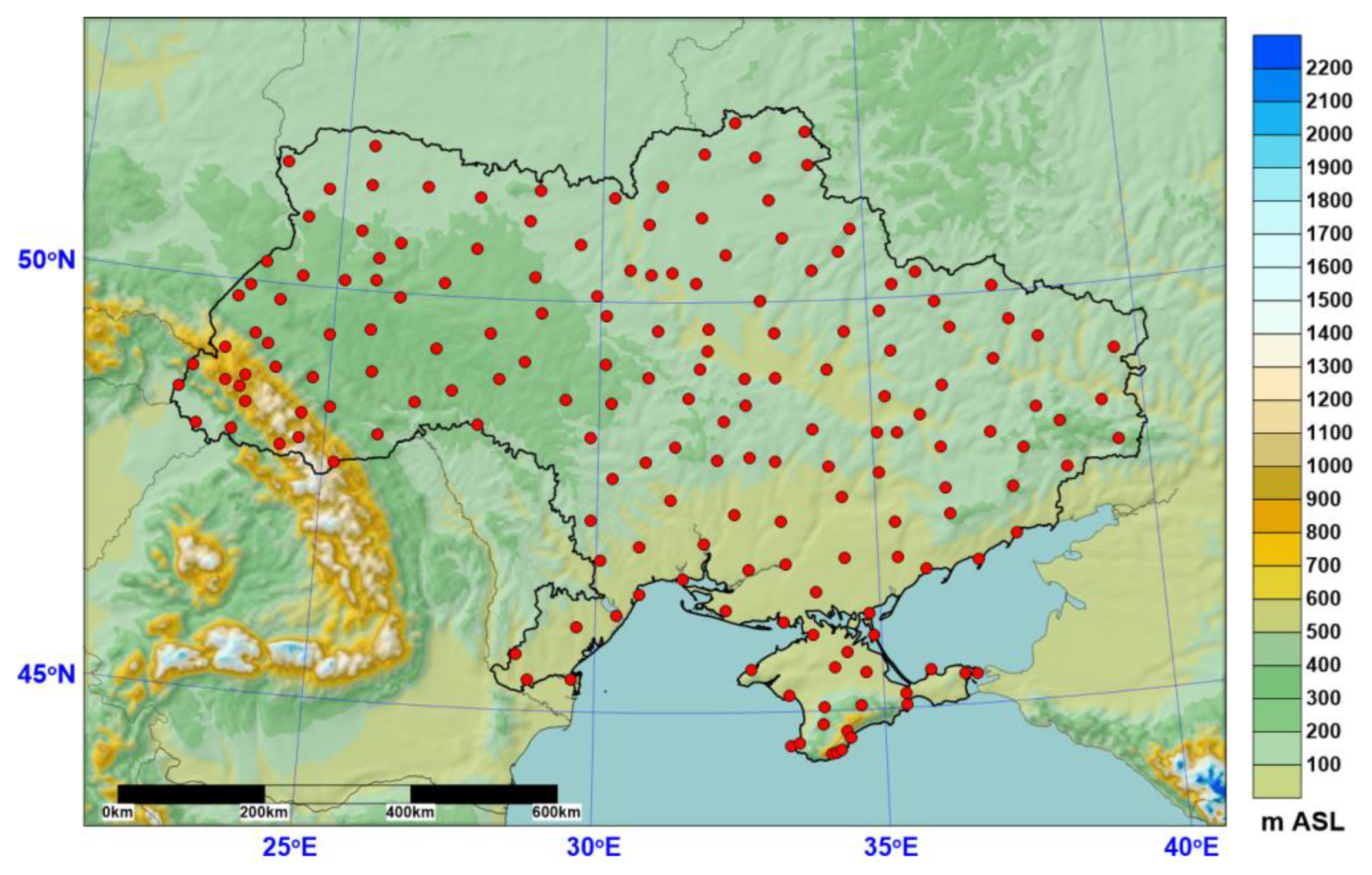
2.1. Domain and Reference Station Data

Figure 1 shows the extended domain of Ukraine and its topography. However, all calculations were strictly performed over the country’s territory, excluding the adjacent areas. The domain is characterized by a variety of climate conditions due to the large south-to-north extent of the territory, along with the complex terrain and the presence of the warm Black Sea and Sea of Azov [30]. The topographic features are primarily due to the Ukrainian part of the Carpathians and the Crimean Mountains, with elevations reaching up to 2061 and 1545 m above sea level, respectively. The rest of the country, in contrast, is relatively flat.

In order to achieve our objectives, high-quality reference data are necessary. For this purpose, we utilized a dataset of 178 quality-controlled and homogenized station time series recently developed for Ukraine [31,32]. The dataset spans the period from 1946 to 2020 (75 years) and includes daily values of the four essential climate variables: atmospheric precipitation, and the minimum, mean, and maximum air temperature. The data development followed the recommendations of the World Meteorological Organization (WMO) [10] and involved several key steps, such as data rescue to fill missing values in the raw time series, thorough quality control to detect and correct or remove errors, and relative homogenization to remove artificial station signals, which are not related to climate. After the data rescue procedure, the quantity of missing data in each time series was less than 5% of the total series length. The quality control was performed by means of the well-established and widely used modern software tools INQC [33] and Climatol [34]. INQC applies an absolute approach, detecting errors within individual time series based on physical principles, thresholds, and statistical analysis. Climatol uses a relative approach, identifying outliers by comparing a candidate series to a reference series constructed from neighboring stations. Multiple iterations were performed with both packages, verifying errors against paper sources and correcting when confirmed. The Climatol software was also used for the relative homogenization of daily station time series. To detect break points, the software employs the standard normal homogeneity test (SNHT), which is applied iteratively—both to the entire series and via a moving window—to minimize false detections, as it is designed to identify only one break at a time. Detected shifts are adjusted using an orthogonal (type II) linear regression model. To homogenize the daily station time series, several Climatol algorithms were tested [31]. The final homogenization results [32] were achieved using a unified collection of break points, developed based on the testing outcomes, and previously collected metadata. Note that according to the HW definition used in our study (see the relevant section below) only the daily maximum air temperature data (TX) were utilized for HW calculations.

Figure 1 illustrates the spatial locations of the 178 meteorological stations whose TX records were used in the study. These stations constitute the basis of the modern monitoring network of Ukraine. As shown in the figure, the stations cover the country’s territory with a relatively high density; for instance, the average distance between the stations is approximately 50 km.

2.2. Gridded Datasets Used for HW Metric Calculations

In our study, we utilized gridded datasets of daily maximum air temperature, which are freely available on the Internet. It is worth noting that we selected only datasets that cover the entire territory of Ukraine and have a temporal span of at least six decades, extending as close as possible to recent years. Such a time period is optimal for our analysis. On the one hand, it is not excessively long, which helps avoid historical data of lower quality. On the other hand, it is sufficiently long to derive a reliable HW climatology and compute consistent trends reflecting recent climate change.

Table 1. Gridded datasets used to evaluate the HW metric sensitivity/uncertainty.

#	Name	Temporal Coverage	Spatial Resolution, lon × lat	Reference
1	ClimUAd	1946–2020	0.1° × 0.1°	[32,35]
2	E-OBS	1950 to present	0.1° × 0.1°	[36]
3	ERA5	1940 to present	0.25° × 0.25°	[37]
4	ERA5-Land	1950 to present	0.1° × 0.1°	[38]
5	20CRV2c	1850–2014	2° × 2°	[39]
6	20CRV3	1806–2015	1° × 1°	[39,40]
7	NCEP-NCAR R1	1948 to present	2.5° × 2.5°	[41]

summarizes the daily gridded datasets used in this study, with brief descriptions provided below.

(1) ClimUAd observation-based daily gridded data of Ukraine [32,35]. The quality-controlled and homogenized station data presented above were used to generate gridded time series with a spatial resolution of 0.1° in both longitude and latitude. The gridding was conducted using the MISH software [42], which is widely applied in climatological researches. The time coverage matches that of the corresponding station series, spanning 1946–2020. The data are freely available for download from the data repository of the Ukrainian Hydrometeorological Institute (https://uhmi.org.ua/eng/data_repo/; accessed on 30 November 2024).

(2) E-OBS v28.0 (E-OBS) observational-based daily gridded data for Europe [36]. The E-OBS dataset is based on the European Climate Assessment & Dataset (ECA&D) collection of station series and is provided as ensemble data (comprising ensemble mean and 20 members) at spatial resolutions of 0.1° × 0.1° and 0.25° × 0.25°. In our analysis, only the ensemble mean data at a 0.1° resolution were used. The dataset covers the period from 1950 to the present. The E-OBS TX dataset was obtained from the Copernicus Climate Data Store (CDS) (https://cds.climate.copernicus.eu; accessed on 30 November 2024).

(3) ERA5 single-level (ERA5) 2 m air temperature data [37]. ERA5 is the latest (fifth generation) global reanalysis product created by the European Center for Medium-Range Weather Forecast (ECMWF). The spatial resolution of the ERA5 single-level reanalysis data is 0.25° × 0.25° (longitude and latitude), with the temporal resolution of 1 h. Since HW metrics in our study are calculated based on TX daily data, the hourly air temperatures were converted to daily maximum values using the CDO software [43]. This conversion was performed by extracting the maximum value from twenty-four hourly records for each day. The ERA5 data cover the period from January 1940 to the present and they were obtained from the Copernicus CDS.

(4) ERA5-Land 2 m air temperature data [38]. ERA5-Land is a refined version of the ERA5 global reanalysis, specifically designed for land surface applications. The spatial resolution of the data is 0.1° × 0.1° (longitude and latitude), while the temporal resolution is the same as in ERA5 (1 h). The conversion of the hourly ERA5-Land temperature data to daily maximum values was performed in a similar manner to the conversion for the ERA5 single-level data. The temporal coverage of ERA5-Land is from January 1950 to the present. Similarly to E-OBS and ERA5, the ERA5-Land TX dataset was downloaded from the Copernicus CDS.

(5) NOAA-CIRES 20th Century Reanalysis V2c (20CRV2c) [39]. 20CRV2c is global reanalysis data developed in the frame of the Twentieth Century Reanalysis Project (20CR), an international effort led by the Physical Sciences Laboratory (PSL) of the National Oceanic and Atmospheric Administration (NOAA) and the Cooperative Institute for Research in Environmental Sciences (CIRES) at the University of Colorado. The V2c version of this dataset has a spatial resolution of 2° × 2° and covers the period from 1850 to 2014. The 20CRV2c daily maximum air temperature data are provided by the NOAA PSL and they were downloaded from their website (https://psl.noaa.gov/data/gridded/data.20thC_ReanV2c.html; accessed on 30 November 2024).

(6) NOAA-CIRES-DOE 20th Century Reanalysis V3 (20CRV3) [39,40]. 20CRV3 is the latest version of the global reanalysis data developed as a part of the 20CR project. This version features a refined spatial resolution of 1° × 1° and the extended temporal coverage from 1836 to 2015, with an additional experimental extension for the period 1806–1835. The 20CRV3 reanalysis daily TX data are provided by the NOAA PSL and they were downloaded from their website (https://psl.noaa.gov/data/gridded/data.20thC_ReanV3.html; accessed on 30 November 2024).

(7) NCEP-NCAR Reanalysis 1 (NCEP-NCAR R1) [41]. The NCEP-NCAR R1 is a global gridded dataset developed by the National Centers for Environmental Prediction (NCEP) and the National Center for Atmospheric Research (NCAR). The dataset has a spatial resolution of 2.5° × 2.5° and covers the period from 1948 to the present. The NCEP-NCAR R1 daily maximum temperature data are provided by the NOAA PSL and they were downloaded from their website (https://psl.noaa.gov/data/gridded/data.ncep.reanalysis.html; accessed on 30 November 2024). It is worth noting that in the downloaded data files of two reanalyzes, 20CRV2c and NCEP-NCAR R1, the spatial resolution is slightly finer (~1.875° × 1.905°) compared to what is declared on the download webpages.

Most of the gridded products used in this study are regularly updated, with the exception of the two versions of the 20CR global data and ClimUAd. The latter is planned to be updated at least once every several years. The usage of 20CRV2c and 20CRV3 is important despite their relatively coarse spatial resolutions (2° × 2° and 1° × 1°, respectively) and the fact that they are no longer updated. Based on their statistical comparison with real measurements for a modern period, it will be possible also to assess approximately their applicability for studying HWs over Ukraine or similar European regions during the XIX century (starting from 1806/1850).

As shown in Table 1, the overlapping period with available TX records across all datasets is 1950–2014 (65 years). Consequently, all HW calculations were performed for this period. In addition, the datasets differ in spatial resolution. To facilitate further calculations and enable mutual comparison, we selected a regular longitude–latitude 0.1° × 0.1° grid (used in ClimUAd and ERA5-Land) as a target one. All other datasets were remapped to this grid using the CDO software with a bilinear interpolation algorithm. It is worth noting that the E-OBS data also have a spatial resolution of 0.1° × 0.1°, but their grid is slightly spatially shifted compared to ClimUAd and ERA5-Land (by ~0.05° along the longitude and latitude). Consequently, the CDO bilinear remapping was applied to E-OBS as well. We believe that such a remapping does not significantly distort the original gridded data.

Finally, all seven datasets—original (ClimUAd and ERA5-Land) and remapped (E-OBS, ERA5, 20CRV2c, 20CRV3, and NCEP-NCAR R1)—were combined to create a mini statistical ensemble of different realizations of the TX variable. Using this ensemble, HW metrics were calculated for each grid point within the territory of Ukraine and for each individual member of the ensemble.

2.3. Heatwave Calculation Methodology

There are many different approaches to defining (or detecting) HW events and, consequently, to quantifying their peculiarities (e.g., [44,45,46,47]). In our study, we adopted the methodology summarized by Perkins and Alexander [1], which is frequently utilized in climatological studies. This methodology typically involves the use of both the daily minimum (TN) and maximum (TX) air temperatures in HW calculations. However, given the objectives of our study, the use of TX data alone is entirely sufficient. The methodology is generally based on applying a relative threshold (which varies by geographical location) for air temperature and identifying instances when the temperature exceeds this threshold. The threshold is calculated for each calendar day of a year by applying a 15-day window (7 days before and 7 days after the given day). This used approach allows us to detect periods with significantly abnormal, positive temperature anomalies throughout the entire year.

Thus, following [1], we define a heatwave as an event when TX exceeds the 90-th percentile threshold (calculated based on the WMO standard 1961–1990 reference period) for at least three consecutive days, allowing for a one-day gap. Perkins and Alexander [1] recommend considering several HW metrics/aspects calculated on a yearly basis, namely the following: heatwave number (HWN), heatwave duration (HWD), heatwave frequency (HWF), heatwave amplitude (HWA), and heatwave magnitude (HWM). In our study, we used the first four metrics. HWN refers to the yearly number of the observed heatwave episodes, with units in [events]; HWD represents the length of the longest yearly HW event, measured in [days]; HWF denotes the yearly sum of heatwave days, measured in [days]; and HWA is a maximum intensity of the hottest yearly event, measured in [°C]. Note that HW intensity is defined as the difference between TX and the corresponding value of the climatological seasonal cycle. All calculations of HW metrics were performed using the R package heatwaveR [48]. Figure 2 illustrates a simple example of calculated HW metrics for one of the Ukrainian stations for 1946.

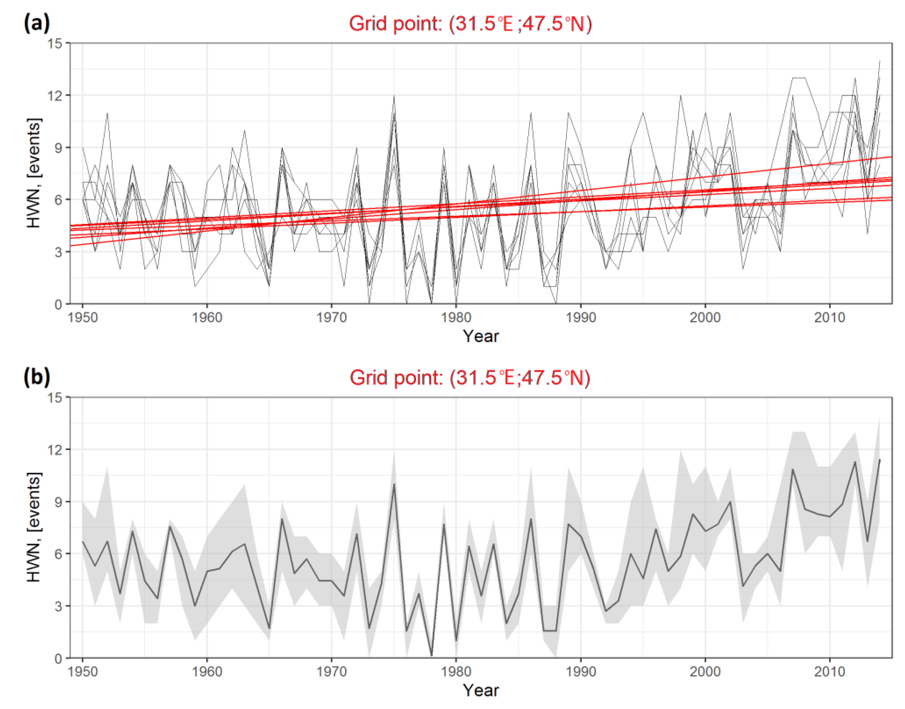
2.4. Quantification of the Sensitivity of HW Metrics to Input Gridded Datasets and Their Comparison with Station-Based Calculations

The sensitivity of HW metrics to the input datasets results in a range (or spread) of metric values calculated for each year and grid point. Any statistical metric characterizing the width of this range can be considered as a measure of sensitivity or, more broadly, a measure of the uncertainty originating from the choice of the input gridded data. For example, Figure 3a illustrates the yearly time series of one HW metric (HWN) calculated for each member of the created statistical ensemble at a selected grid point located in a relatively flat area of the domain (in the south-eastern part of Ukraine). Additionally, linear trends for each HWN time series, calculated using Sen’s approach [49]—a nonparametric and robust method resistant to gross errors/outliers—are also shown. To quantify the spread of HWN values (and hence the uncertainty of the metrics) for each year of the period, we calculate the ranges between the maximum and minimum values of the HW metric (Max–Min). Such ranges, along with the ensemble mean time series of the HWN metric, are presented in Figure 3b, which corresponds to the same grid point as Figure 3a. Due to the yearly variations in the Max–Min values, which are clearly seen in Figure 3b, it is more convenient to use in the analysis their mean value, averaged over the entire period. A similar Max–Min range is also calculated for the slopes of the linear trends (no additional averaging is performed in this case). Thus, the Max–Min (averaged over time for HW metrics and unaveraged for trend slopes) serves as the primary variable in our study to quantify the sensitivity or uncertainty associated with the input gridded data. It is important to note that this method does not use HW calculations derived from station time series, which are typically considered as reference results. Consequently, such a sensitivity or uncertainty quantification can be regarded as absolute (not tied to reference measurements) and is applicable in regions where high-quality observational data are lacking.

The second approach, aligned with the research goals, aims to compare HW metrics calculated from the gridded datasets with corresponding results obtained from the reference station series. To facilitate statistical comparison, the gridded data were additionally interpolated to the station locations using the nearest neighbor method. The relatively high spatial resolution of all gridded datasets (0.1° × 0.1°, approximately 10 km in both longitude and latitude) minimizes interpolation errors. The comparison involved calculating several statistical verification indices: mean error (BIAS), root mean square error (RMSE), Pearson’s correlation coefficient (R), and the difference between the trend slopes derived from station and gridded data (TrD). The formulas for the first three indices are well established and can be found, for instance, in [50]. The formula for TrD is evident from its introduction above. The verification indices were computed for each HW metric, each gridded dataset, and each climate station. The results were then aggregated into box plots to illustrate statistical distributions of the verification indices.

3. Results and Discussion

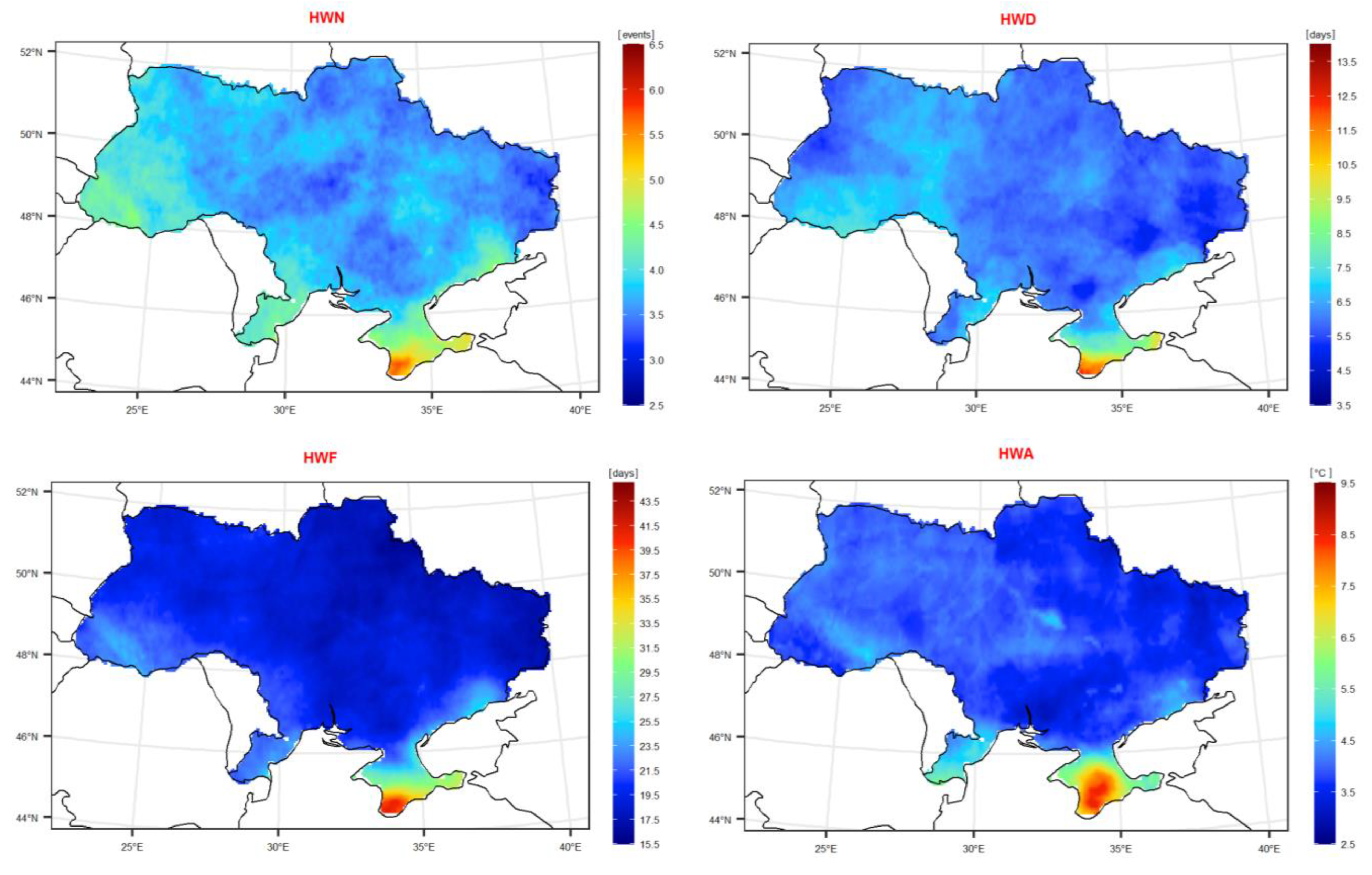
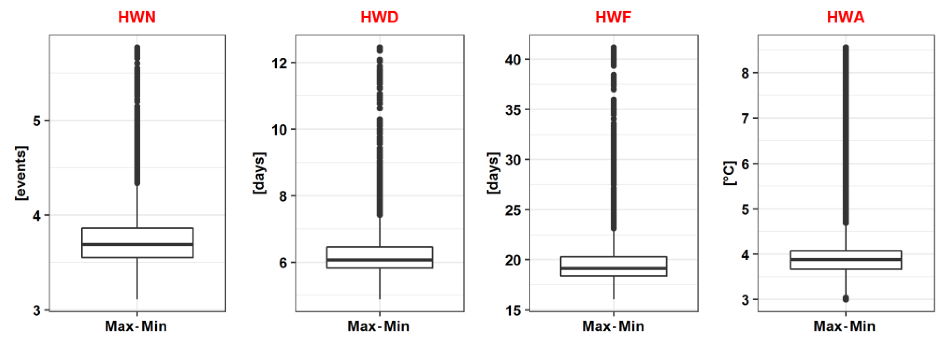
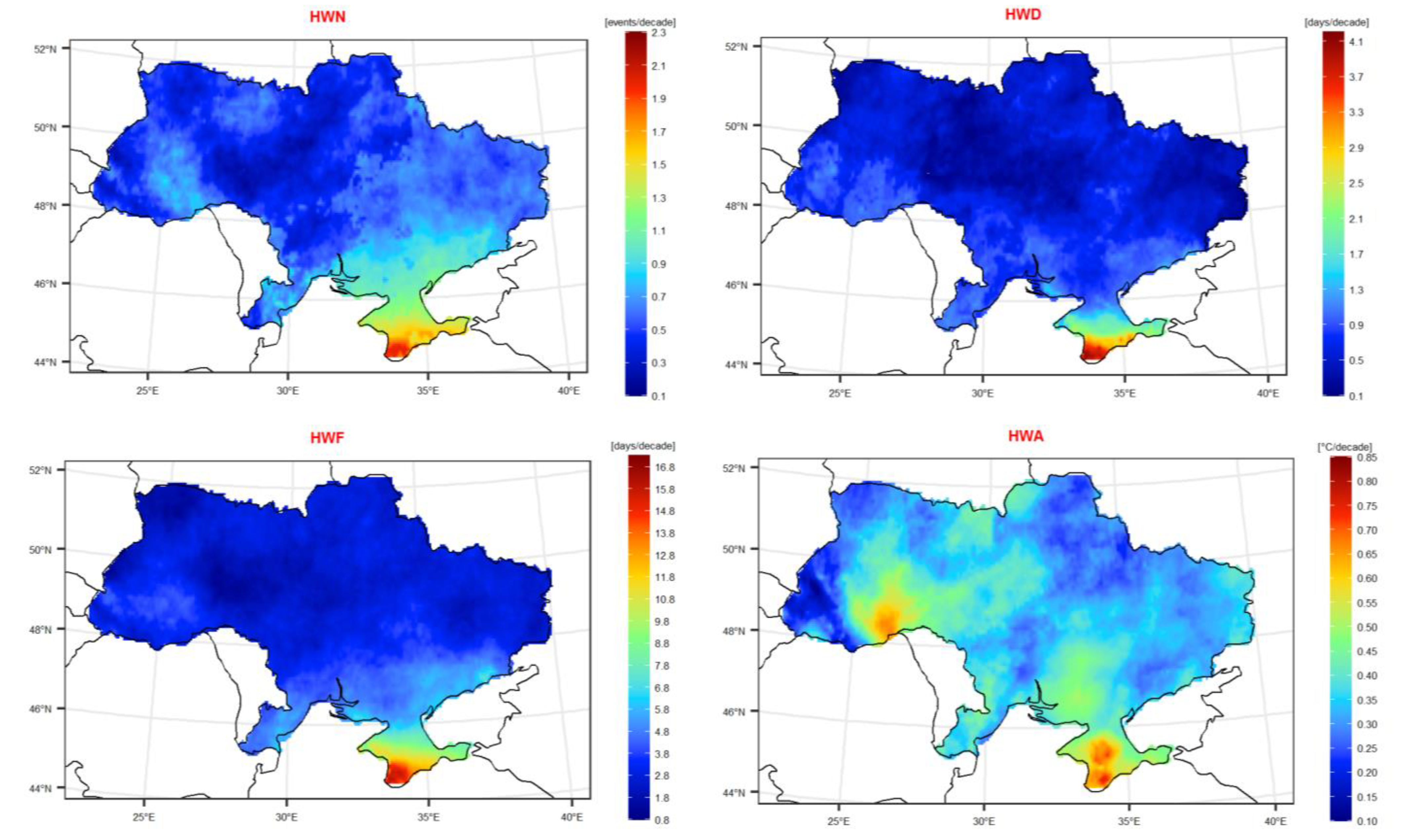
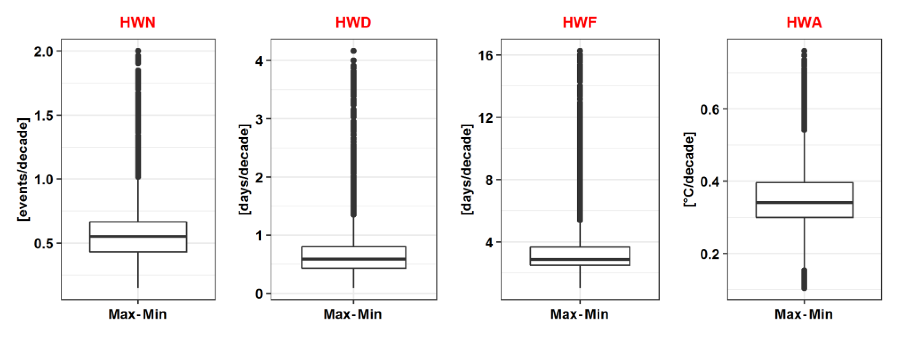
3.1. Absolute HW Metrics Sensitivity/Uncertainty Quantification

The spatial distribution of the Max–Min ranges, calculated for the HW metrics and averaged over 1950–2014, is shown in Figure 4, while their aggregated representations as box plots are presented in Figure 5. Similar results for the slopes of Sen’s linear trends, identified in the yearly time series of the HW metrics, are displayed in Figure 6 and Figure 7.

As shown in Figure 4, the spatial distribution patterns of the Max–Min values over Ukraine are relatively homogeneous for all four HW metrics. The only region with substantially higher Max–Min values is the Crimea Peninsula. Additionally, the Carpathian Mountains and the area closest to the coastline also exhibit a slightly greater variability in HW metrics derived from the different gridded datasets. This is likely due to the influence of complex topography and/or the presence of large water bodies. The original spatial resolution of some gridded datasets (e.g., 20CRV2c, 20CRV3, and NCEP-NCAR R1) is relatively coarse, which makes it challenging for these datasets to capture the fine spatial structure of the temperature field, including its extreme values, in such regions. This limitation is reflected in the calculated HW metric and, consequently, in their Max–Min ranges.

It is also worth noting that, starting from the mid-1980s, the variability of HW metrics calculated from different input gridded datasets began to increase substantially in the Crimea Peninsula, with the largest contribution from NCEP-NCAR R1. This reanalysis significantly overestimates (compared to other datasets) two HW metrics, HWD and HWF, and underestimates HWA. Across the entire country, the main contributors to the spread of HW metric values are reanalyzes with the coarsest spatial resolution, namely 20CRV2c, 20CRV3, and NCEP-NCAR R1. Time series of three HW metrics (HWN, HWD, and HWF) derived from these reanalyzes exhibit significantly greater temporal variability than those from other gridded datasets. These reanalyzes produce both the highest and lowest metric values in most years of the study period. As mentioned above, the largest variability is observed in the southern part of Ukraine, particularly on the Crimea Peninsula, and during the last 30 years of the 1950–2014 period. However, HWA follows a slightly different pattern. In this case, 20CRV3 (and 20CRV2c from the mid-1980s onward) shows an underestimation (cold bias) compared to other datasets. This finding aligns with the results of (Figure S13 in [29]), where a similar underestimation was observed on a global scale for the ETCCDI index TXx (annual maximum of the daily maximum air temperature; closely related to HWA) derived from the same reanalysis. The tipping point observed in the mid-1980s in HW metric time series calculated from 20CRV2c, 20CRV3, and NCEP-NCAR R1 is likely attributed to changes in data sources and assimilation techniques used in these reanalyzes [39,41].

Overall, as indicated by the box plots in Figure 5, the ranges of Max–Min values for HW metrics over Ukraine are as follows: HWN (3.1; 5.8) with a mean value of 3.7 [events]; HWD (4.9; 12.6) with a mean of 6.0 [days]; HWF (15.8; 42.1) with a mean of 19.1 [days]; and HWA (3.0; 8.6) with a mean of 3.9 [°C]. These results suggest that, even after time averaging Max–Min values over the study period (1950–2014), the sensitivity of HW metrics to the input gridded data remains relatively high. In terms of HW climatology uncertainty arising from the input gridded datasets, these findings indicate a considerable variability. For example, the number of detected HW episodes may differ by approximately four events depending on the gridded dataset used, while the total duration of HWs and the duration of the most intense HWs may vary by 19 and 6 days, respectively. Regarding HW amplitude, TX deviations from the climatological annual cycle during HW events could differ by approximately 4 °C. Such significant differences should be kept in mind when evaluating and quantifying consequences of past HW events based on different gridded datasets, particularly in sectors like the economy or public health. Based on these results, we recommend, similar to [25], that in the absence of reliable station measurements needed for verification purposes, HW climatology calculations should incorporate several gridded products. This approach can help assess the climatology uncertainty and provide insights into the inherent limitations of gridded datasets in reproducing the air temperature extremes.

As demonstrated in Figure 6, the spatial distributions of Max–Min ranges for the trend slopes of HW metrics are similar to those in Figure 4. However, the influence of the Carpathian Mountains on trend slope variations is less pronounced compared to the HW metrics themselves. Additionally, relatively larger variability in Max–Min values for HWA trends is observed in the pre-Carpathian region (western Ukraine). Overall, the ranges of Max–Min values for the HW metrics trends across Ukraine are as follows (Figure 5): HWN (0.1; 2.0) with a mean value of 0.6 [events/decade]; HWD (0.1; 4.2) with a mean of 0.7 [days/decade]; HWF (0.9; 16.2) with a mean of 2.9 [days/decade]; HWA (0.1; 0.8) with a mean of 0.3 [°C/decade]. These findings indicate that when using different input gridded datasets, the estimated regular changes of HWN may differ by approximately 0.6 [events/decade]. Similarly, trend slope estimates for HWD, HWF and HWA may vary by about 0.7 [days/decade], 2.9 [days/decade] and 0.3 [°C/decade], respectively.

The quantitative evaluation of the uncertainty of HW metrics and their trends shows that the variability in HW metric trend slopes (their sensitivity to input datasets) is slightly lower compared to the metrics themselves. Such reduced variability in trends likely indicates that the time series of HW metrics derived from different gridded data should be coherent, showing relatively consistent over- or underestimation of each other over time. This conclusion (regarding HWA) aligns with the findings obtained in [29], where the authors indicated that while there is sometimes a large spread in the absolute values of ITCCDI temperature indices derived from different reanalysis products, their long-term trends are in agreement.

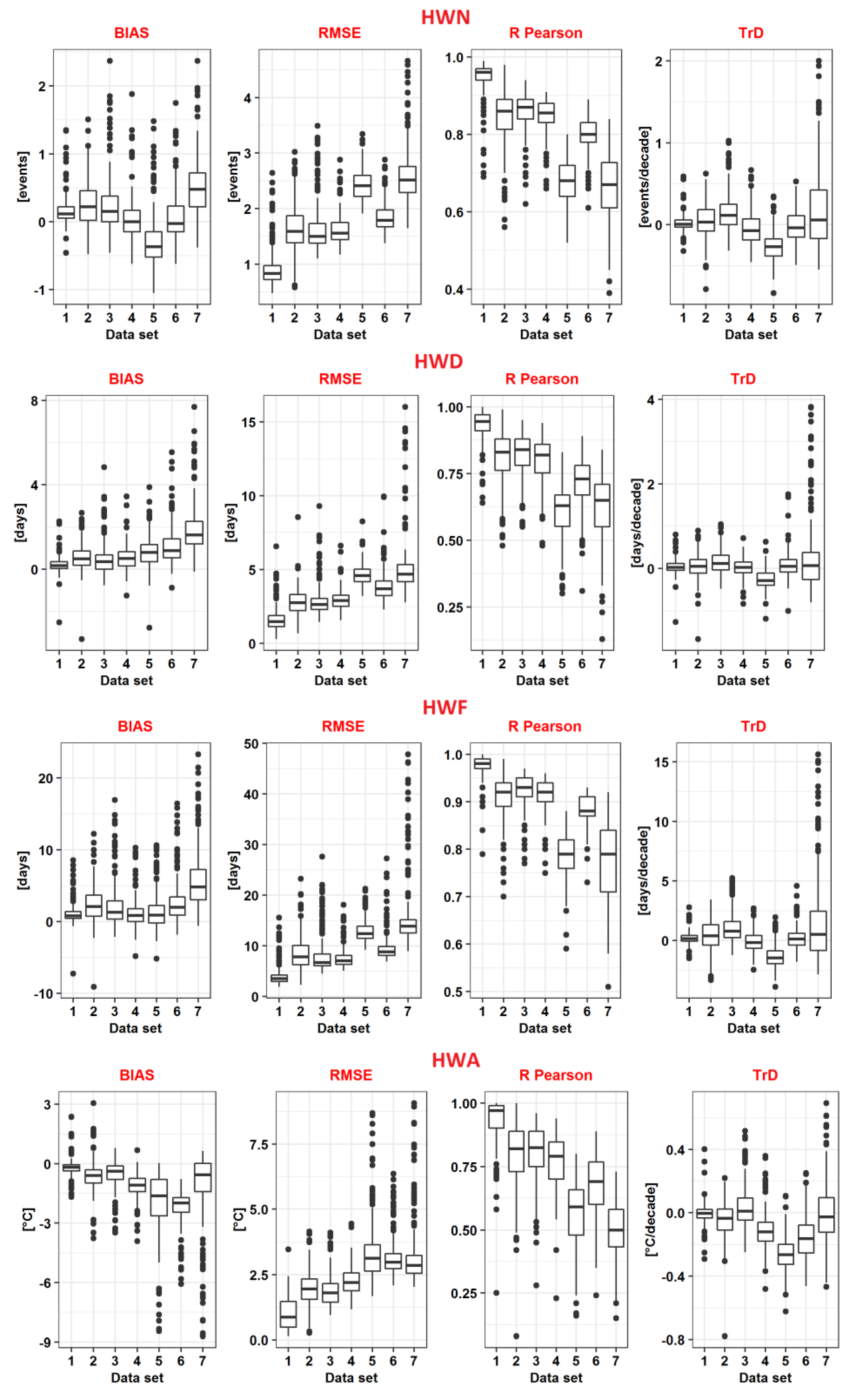
3.2. Verification of HW Metrics Against the Reference Station Data

Figure 8 presents box plots of the verification statistics, illustrating compatibility between the HW climatology calculated from gridded datasets and reference station data. The statistics were calculated on a station basis and then aggregated into box plots for each HW metric. The average values of these statistics, calculated across all stations, are summarized in

Table 2. Verification statistics (averaged values over all stations). The BIAS and RMSE are measured in the same units as the HW metric, R Pearson is dimensionless, and TrD is measured in [HW metric]/decade.

HW Metric	Verification Statistic	Dataset
		ClimUAd	E-OBS	ERA5	ERA5-Land	20CRV2c	20CRV3	NCEP-NCAR R1
HWN, [events]	BIAS	0.16	0.26	0.25	0.05	−0.29	0.07	0.49
	RMSE	0.92	1.64	1.63	1.64	2.44	1.85	2.61
	R Pearson	0.95	0.85	0.86	0.84	0.68	0.80	0.66
	TrD	0.02	0.03	0.14	−0.05	−0.26	−0.03	0.20
HWD, [days]	BIAS	0.23	0.58	0.50	0.53	0.83	1.11	1.86
	RMSE	1.62	2.83	2.89	2.97	4.63	3.89	5.22
	R Pearson	0.93	0.81	0.82	0.80	0.61	0.71	0.62
	TrD	0.04	0.06	0.16	0.02	−0.27	0.08	0.26
HWF, [days]	BIAS	1.12	2.45	2.24	1.18	1.49	2.87	5.76
	RMSE	4.04	8.52	8.21	7.60	13.08	9.82	15.81
	R Pearson	0.97	0.91	0.92	0.91	0.78	0.88	0.77
	TrD	0.17	0.39	0.99	−0.14	−1.37	0.16	1.56
HWA, [°C]	BIAS	−0.19	−0.64	−0.55	−1.13	−1.98	−2.29	−1.14
	RMSE	0.97	1.95	1.89	2.25	3.41	3.20	3.25
	R Pearson	0.93	0.80	0.81	0.77	0.56	0.68	0.49
	TrD	−0.01	−0.05	0.03	−0.10	−0.26	−0.16	0.00

. Generally, as shown in Figure 8, all HW metrics exhibit similar patterns in the distribution of the verification statistics. The best verification results were obtained from ClimUAd. However, this is not surprising, as the same station time series were used both to create ClimUAd and to conduct an evaluation study. The E-OBS, ERA5, and ERA5-Land gridded datasets show comparable verification results for all HW metrics. For example, for HWN, the calculated statistics—BIAS, RMSE, Pearson’s R, and TrD—are close to 0.0 [events], 1.7 [events], 0.9, and 0.0 [events/decade], respectively, across all three datasets. Similar verification results are observed for the other HW metrics (Table 2). This indicates that any of these datasets can be used to study HW climatology in Ukraine, neighboring countries, and potentially in other European domains with a similar-to-Ukraine climate and terrain features with comparable accuracy.

However, it is worth noting that E-OBS, as an observation-based gridded dataset, may produce completely different evaluation results when applied to other European domains. The accuracy of E-OBS depends heavily on station data used for gridding (e.g., the number of stations, percentage of missing values, and overall data quality), which can vary significantly across regions. Consequently, in other domains, verification results for this dataset could be better, potentially approaching the performance of ClimUAd observed in our study.

The verification statistics for 20CRV3 are less favorable than those for the E-OBS, ERA5, and ERA5-Land datasets but are significantly better than those for the 20CRV2c and NCEP-NCAR R1 reanalysis. For example, for HWN, the mean values of the verification statistics—BIAS, RMSE, Pearson’s R, and TrD—are approximately 0.0 [events], 1.9 [events], 0.8, and 0.0 [events/decade], respectively. Thus, the 20CRV3 dataset is suitable for studying HW climatology in past historical periods (e.g., 19th and early 20th centuries) with reasonable accuracy.

It is interesting to note that all datasets showed an average overestimation of HWN, HWD, and HWF compared to the station data, with the only exception of HWN derived from 20CRV2c. Unfortunately, we have not found scientific publications that compare reanalysis-based HWN, HWD, and HWF to corresponding station calculations and report similar biases. A likely reason for the overestimation can be the relatively coarse spatial resolution of the gridded datasets, which can lead to spatial smoothing of temperature extremes. This can artificially extend the duration and frequency of heatwaves since localized cooling effects are not well captured. Additionally, the applied HW definition relies on TX 90-th percentile thresholds, which are calculated based on the 1961–1990 reference period using data from the same dataset serving as input. Differences in these thresholds may contribute to variations in the calculated metrics, potentially leading to an overestimation of the number, duration, and frequency of heatwaves. Further research is needed to identify the calculation factors responsible for these discrepancies.

While HWN, HWD, and HWF are generally overestimated, all datasets exhibited a cold bias for HWA, indicating an underestimation of heatwave intensity. The largest average cold biases for HWA were calculated based on 20CRV3 and 20CRV2c: −2.23 and −1.98 °C, respectively. ERA5-Land underestimated HWA with almost the same bias as NCEP-NCAR R1 (−1.13 °C), whereas ERA5 showed a better agreement with station data (−0.55 °C), comparable with the observation-based gridded datasets (ClimUAd and E-OBS). These results are consistent with findings reported in [25,29], where the authors compared TX (or TXx) derived from reanalysis products (including ERA5 and 20CRV3) with observation-based data on a global scale and found a significant underestimation of the maximum air temperature, particularly in mountainous regions [25].

The calculated average values of RMSE for all HW metrics revealed substantially larger scatter errors in metrics derived from reanalyzes with the coarsest spatial resolution (20CRV2c and NCEP-NCAR R1) compared to other datasets. While 20CRV3 exhibited a smaller RMSE than 20CRV2c and NCEP-NCAR R1, it still showed significantly larger errors compared to ClimUAd, E-OBS, ERA5, and ERA5-Land. These findings support the previously stated conclusion regarding the greater variability of HW metric time series calculated from the reanalyzes with the coarse resolution. Similar conclusions hold for the Pearson correlation between HW metrics derived from the gridded data and station measurements. The weakest correlation was found for 20CRV2c and NCEP-NCAR R1 for all HW metrics. Notably, the average Pearson correlation coefficients calculated for HWA from ERA5 and 20CRV3 are comparable to the results obtained in [29], where a similar correlation between TXx values derived from the same reanalysis and HadEX3 was evaluated at a global scale. The authors found that the globally averaged correlation is 0,64 and 0.62 for ERA5 and 20CRV3, respectively, whereas for Ukraine we obtained 0.81 and 0.68. The differences may partly stem from variations in metric/index definitions or from differences in spatial domains and temporal periods used in the averaging.

It is important to emphasize that the findings of this study are based on a limited geographical domain. However, this limitation is unavoidable, as we completely rely on the available verification data. At the same time, Ukraine is a relatively large country—the second largest in Europe—encompassing a diverse range of climate conditions and terrain features [30]. Its geography includes warm seas, mountain ranges, and even a desert. Given this diversity, we believe that the conclusions drawn from this study can be extended to other European regions, particularly to neighboring countries and areas with similar climatic conditions, such as Central and Eastern Europe. The indirect comparison performed above supports this conclusion. However, unfortunately, we have not found studies that report similar verification statistics for the HW metrics in other European regions, which could directly support the broader applicability of our results.

4. Conclusions

In this research, based on a case study of Ukraine, we examined the sensitivity of HW climatology to input gridded datasets commonly used in climate research. To achieve this, we created a mini statistical ensemble of gridded daily data, comprising seven different realizations of the TX variable for Ukraine. The approach, summarized by Perkins and Alexander [1], was applied to determine the yearly time series of four heatwave metrics, HWN, HWD, HWF, and HWA, for the period 1950–2014. The uncertainty of HW climatology was quantified by calculating the intervals between the minimum and maximum values of the metrics (Max–Min ranges) derived from the different gridded datasets.

The average Max–Min intervals, computed over time (1950–2014) and space (Ukraine), were as follows: HWN 3.7 [events], HWD 6.0 [days], HWF 19.1 [days], and HWA 3.9 [°C], indicating a notable level of uncertainty in HW metrics. Geophysical terrain features, such as mountainous regions and large water bodies, were found to amplify the metric spreads. Additionally, similar Max–Min ranges were calculated for the slopes of Sen’s linear trends in HW metric time series. However, the sensitivity of the trends to gridded datasets was notably lower compared to the sensitivity of the HW metrics themselves. The Max–Min intervals for the trends, averaged over time (1950–2014) and space (Ukraine), were determined as follows: HWN 0.6 [events/decade], HWD 0.7 [days/decade], HWF 2.9 [days/decade], and HWA 0.3 [°C/decade]. Our findings suggest that in the case of the absence of reliable station measurements needed for verification, HW climatology calculations should involve several gridded products. This approach can facilitate the evaluation of the climatology uncertainty and provide insights into the inherent limitations of gridded datasets in reproducing the air temperature extremes.

The HW metrics and their trends calculated from the gridded datasets were also compared with those derived from high-quality station time series recently developed for Ukraine. Several statistical metrics were employed to assess the compatibility between the gridded and station-based HW calculations. The best estimates of HW climatology were obtained from ClimUAd, which is unsurprising given that ClimUAd was developed using the same collection of station series that were used for the verification study. The E-OBS, ERA5 and ERA5-Land gridded data demonstrated similar verification statistics, indicating that any of these datasets can be used to study HW climatology with comparable accuracy. In contrast, the verification statistics for 20CRV3 were worse than those for E-OBS, ERA5 and ERA5-Land but significantly better than for 20CRV2c and NCEP-NCAR R1 reanalysis. Consequently, 20CRV3 is more suitable for defining HW climatology in historical periods, particularly for the 19th and early 20th centuries.

Unfortunately, we have not found previously published studies which can be used for a direct comparison of our results. The number of publications verifying HW metrics (HWN, HWD, HWF, and HWA) derived from gridded datasets, including reanalysis, is rather limited. However, some indirect comparisons indicated consistency with several studies that have evaluated extreme air temperatures derived from various reanalysis products against observation-based data, supporting the potential ability to extend the findings beyond Ukraine.

Reliable HW climatology is vitally important for climate risk assessment and the development of mitigation measures and strategies for extreme temperature events. By comparing HW metrics derived from gridded data with calculations from high-quality station time series, the research underlines the need for careful dataset selection in climate studies. By identifying the most appropriate datasets for HW assessment in Ukraine (which can be extended for other spatial domains, at least, for neighboring countries and potentially across Europe), this work contributes to improving the accuracy of climate research and supports better-informed adaptation and mitigation strategies in the face of growing climate extremes.

References

1. Perkins, S.E.; Alexander, L.V. On the measurement of heat waves. J. Clim. 2013, 26, 4500–4517. [Google Scholar] [CrossRef]
2. Campbell, S.; Remenyi, T.A.; White, C.J.; Johnston, F.H. Heatwave and health impact research: A global review. Health Place 2018, 53, 210–218. [Google Scholar] [CrossRef]
3. Perkins-Kirkpatrick, S.E.; Lewis, S.C. Increasing trends in regional heatwaves. Nat. Commun. 2020, 11, 3357. [Google Scholar] [CrossRef] [PubMed]
4. Yadav, N.; Rajendra, K.; Awasthi, A.; Singh, C.; Bhushan, B. Systematic exploration of heat wave impact on mortality and urban heat island: A review from 2000 to 2022. Urban Clim. 2023, 51, 101622. [Google Scholar] [CrossRef]
5. Shevchenko, O.; Lee, H.; Snizhko, S.; Mayer, H. Long-term analysis of heat waves in Ukraine. Int. J. Climatol. 2014, 34, 1642–1650. [Google Scholar] [CrossRef]
6. Spinoni, J.; Lakatos, M.; Szentimrey, T.; Bihari, Z.; Szalai, S.; Vogt, J.; Antofie, T. Heat and cold waves trends in the Carpathian Region from 1961 to 2010. Int. J. Climatol. 2015, 35, 4197–4209. [Google Scholar] [CrossRef]
7. Lhotka, O.; Kyselý, J. The 2021 European heat wave in the context of past major heat waves. Earth Space Sci. 2022, 9, e2022EA002567. [Google Scholar] [CrossRef]
8. Serrano-Notivoli, R.; Lemus-Canovas, M.; Barrao, S.; Sarricolea, P.; Meseguer-Ruiz, O.; Tejedor, E. Heat and cold waves in mainland Spain: Origins, characteristics, and trends. Weather Clim. Extrem. 2022, 37, 100471. [Google Scholar] [CrossRef]
9. Cimolai, C.; Aguilar, E. Assessing Argentina’s heatwave dynamics (1950–2022): A comprehensive analysis of temporal and spatial variability using ERA5-LAND. Theor. Appl. Climatol. 2024, 155, 4925–4940. [Google Scholar] [CrossRef]
10. Meehl, G.A.; Tebaldi, C. More intense, more frequent, and longer lasting heat waves in the 21st century. Science 2004, 305, 994–997. [Google Scholar] [CrossRef] [PubMed]
11. Molina, M.O.; Sánchez, E.; Gutiérrez, C. Future heat waves over the Mediterranean from an Euro-CORDEX regional climate model ensemble. Sci. Rep. 2020, 10, 8801. [Google Scholar] [CrossRef] [PubMed]
12. Ramarao, M.V.S.; Arunachalam, S.; Sánchez, B.N.; Schinasi, L.H.; Bakhtsiyarava, M.; Caiaffa, W.T.; Dronova, I.; O’neill, M.S.; Avila-Palencia, I.; Gouveia, N.; et al. Projected changes in heatwaves over Central and South America using high-resolution regional climate simulations. Sci. Rep. 2024, 14, 23145. [Google Scholar] [CrossRef] [PubMed]
13. Liu, J.; Wang, A.; Zhang, T.; Pan, P.; Ren, Y. Projected increase in heatwaves under 1.5 and 2.0 °C warming levels will increase the socio-economic exposure across China by the late 21st century. Atmosphere 2024, 15, 900. [Google Scholar] [CrossRef]
14. Aguilar, E.; Auer, I.; Brunet, M.; Peterson, T.C.; Wieringa, J. WMO Guidelines on Climate Metadata and Homogenization; WCDMP No. 53, WMO-TD No. 1186; WMO: Geneva, Switzerland, 2003; p. 55. [Google Scholar]
15. Amou, M.; Gyilbag, A.; Demelash, T.; Xu, Y. Heatwaves in Kenya 1987–2016: Facts from CHIRTS High Resolution Satellite Remotely Sensed and Station Blended Temperature Dataset. Atmosphere 2021, 12, 37. [Google Scholar] [CrossRef]
16. Oliveira, A.; Lopes, A.; Correia, E. Annual summaries dataset of Heatwaves in Europe, as defined by the Excess Heat Factor. Data Brief 2022, 4, 108511. [Google Scholar] [CrossRef] [PubMed]
17. Becker, F.N.; Fink, A.H.; Bissolli, P.; Pinto, J.G. Towards a more comprehensive assessment of the intensity of historical European heat waves (1979–2019). Atmos. Sci. Lett. 2022, 23, e1120. [Google Scholar] [CrossRef]
18. Espinosa, L.A.; Portela, M.M.; Matos, J.P. ERA5-Land reanalysis temperature data addressing heatwaves in Portugal. In INCREaSE 2023. Advances in Sustainability Science and Technology; Semião, J.F.L.C., Sousa, N.M.S., da Cruz, R.M.S., Prates, G.N.D., Eds.; Springer: Cham, Switzerland, 2023; pp. 81–94. [Google Scholar] [CrossRef]
19. Espinosa, L.A.; Portela, M.M.; Moreira Freitas, L.M.; Gharbia, S. Addressing the spatiotemporal patterns of heatwaves in Portugal with a validated ERA5-Land dataset (1980–2021). Water 2023, 15, 3102. [Google Scholar] [CrossRef]
20. Labban, A.; Morsy, M.; Abdeldym, A.; Abdel Basset, H.; Al-Mutairi, M. Assessment of changes in heatwave aspects over Saudi Arabia during the last four decades. Atmosphere 2023, 14, 1667. [Google Scholar] [CrossRef]
21. Fiddes, J.; Gruber, S. TopoSCALE v.1.0: Downscaling gridded climate data in complex terrain. Geosci. Model Dev. 2014, 7, 387–405. [Google Scholar] [CrossRef]
22. Frustaci, G.; Pilati, S.; Lavecchia, C.; Montoli, E.M. High-Resolution Gridded Air Temperature Data for the Urban Environment: The Milan Data Set. Forecasting 2022, 4, 238–261. [Google Scholar] [CrossRef]
23. Sterl, A. On the (In)Homogeneity of Reanalysis Products. J. Clim. 2004, 17, 3866–3873. [Google Scholar] [CrossRef]
24. Ferguson, C.R.; Villarini, G. An evaluation of the statistical homogeneity of the Twentieth Century Reanalysis. Clim. Dyn. 2014, 42, 2841–2866. [Google Scholar] [CrossRef]
25. Coughlan de Perez, E.; Arrighi, J.; Marunye, J. Challenging the universality of heatwave definitions: Gridded temperature discrepancies across climate regions. Clim. Change 2023, 176, 167. [Google Scholar] [CrossRef]
26. Zhang, M.; Yang, X.; Cleverly, J.; Huete, A.; Zhang, H.; Yu, Q. Heat wave tracker: A multi-method, multi-source heat wave measurement toolkit based on Google Earth Engine. Environ. Model. Softw. 2022, 147, 105255. [Google Scholar] [CrossRef]
27. Velikou, K.; Lazoglou, G.; Tolika, K.; Anagnostopoulou, C. Reliability of the ERA5 in replicating mean and extreme temperatures across Europe. Water 2022, 14, 543. [Google Scholar] [CrossRef]
28. Sidău, M.R.; Croitoru, A.-E.; Alexandru, D.-E. Comparative Analysis between Daily Extreme Temperature and Precipitation Values Derived from Observations and Gridded Datasets in North-Western Romania. Atmosphere 2021, 12, 361. [Google Scholar] [CrossRef]
29. Dunn, R.J.H.; Donat, M.G.; Alexander, L.V. Comparing extremes indices in recent observational and reanalysis products. Front. Clim. 2022, 4, 989505. [Google Scholar] [CrossRef]
30. Lipinsky, V.M.; Dyachuk, V.A.; Babichenko, V.M. (Eds.) Climate of Ukraine; Vydavnytstvo Raevskogo: Kyiv, Ukraine, 2003; p. 343. ISBN 966-7016-18-8. (In Ukrainian) [Google Scholar]
31. Skrynyk, O.Y.; Sidenko, V.; Aguilar, E.; Guijarro, J.; Skrynyk, O.A.; Palamarchuk, L.; Oshurok, D.; Osypov, V.; Osadchyi, V. Data quality control and homogenization of daily precipitation and air temperature (mean, max and min) time series of Ukraine. Int. J. Climatol. 2023, 43, 4166–4182. [Google Scholar] [CrossRef]
32. Osadchyi, V.; Skrynyk, O.Y.; Sidenko, V.; Aguilar, E.; Guijarro, J.; Szentimrey, T.; Skrynyk, O.A.; Palamarchuk, L.; Oshurok, D.; Kravchenko, I.; et al. Gridded data of daily atmospheric precipitation and minimum, mean and maximum air temperature for Ukraine, 1946–2020. In Proceedings of the EGU General Assembly 2024, Vienna, Austria, 14–19 April 2024. [Google Scholar] [CrossRef]
33. Aguilar, E. INDECIS Quality Control Software and Manual: INQC, Beta Version. 2019. Available online: http://www.indecis.eu/docs/Deliverables/Deliverable_3.1.a.pdf (accessed on 30 November 2024).
34. Guijarro, J.A. Homogenization of Climatic Series with Climatol. Version 4.0.7. Guide. 2023. Available online: https://www.climatol.eu/climatol4.1.2-en.pdf (accessed on 30 November 2024).
35. ClimUAd: Ukrainian Gridded Daily Air Temperature (Min, Max, Mean) and Atmospheric Precipitation Data (1946–2020). Available online: https://www.uhmi.org.ua/data_repo/ClimUAd_Ukrainian_gridded_daily (accessed on 30 November 2024). [CrossRef]
36. Cornes, R.; van der Schrier, G.; van den Besselaar, E.J.M.; Jones, P.D. An ensemble version of the E-OBS temperature and precipitation datasets. J. Geophys. Res. Atmos. 2018, 123, 9391–9409. [Google Scholar] [CrossRef]
37. Hersbach, H.; Bell, B.; Berrisford, P.; Hirahara, S.; Horányi, A.; Muñoz-Sabater, J.; Nicolas, J.; Peubey, C.; Radu, R.; Schepers, D.; et al. The ERA5 global reanalysis. Q. J. R. Meteorol. Soc. 2020, 146, 1999–2049. [Google Scholar] [CrossRef]
38. Muñoz-Sabater, J.; Dutra, E.; Agustí-Panareda, A.; Albergel, C.; Arduini, G.; Balsamo, G.; Boussetta, S.; Choulga, M.; Harrigan, S.; Hersbach, H.; et al. ERA5-Land: A state-of-the-art global reanalysis dataset for land applications. Earth Syst. Sci. Data 2021, 13, 4349–4383. [Google Scholar] [CrossRef]
39. Compo, G.P.; Whitaker, J.S.; Sardeshmukh, P.D.; Matsui, N.; Allan, R.J.; Yin, X.; Gleason, B.E.; Vose, R.S.; Rutledge, G.; Bessemoulin, P.; et al. The Twentieth Century Reanalysis project. Q. J. R. Meteorol. Soc. 2011, 137, 1–28. [Google Scholar] [CrossRef]
40. Slivinski, L.C.; Compo, G.P.; Whitaker, J.S.; Sardeshmukh, P.D.; Giese, B.S.; McColl, C.; Allan, R.; Yin, X.; Vose, R.; Titchner, H.; et al. Towards a more reliable historical reanalysis: Improvements for version 3 of the Twentieth Century Reanalysis system. Q. J. R. Meteorol. Soc. 2019, 145, 2876–2908. [Google Scholar] [CrossRef]
41. Kalnay, E.; Kanamitsu, M.; Kistler, R.; Collins, W.; Deaven, D.; Gandin, L.; Iredell, M.; Saha, S.; White, G.; Woollen, J.; et al. The NCEP/NCAR 40-year reanalysis project. Bull. Am. Meteorol. Soc. 1996, 77, 437–470. [Google Scholar] [CrossRef]
42. Szentimrey, T.; Bihari, Z. Manual of Interpolation Software MISHv1.03; Hungarian Meteorological Service: Budapest, Hungary, 2014. [Google Scholar]
43. Schulzweida, U.; Climate Data Operators (CDO). Max-Plank Institute for Meteorology. 2023. Available online: https://code.mpimet.mpg.de/projects/cdo (accessed on 30 November 2024).
44. Tong, S.; Wang, X.Y.; Barnett, A.G. Assessment of heat-related health impacts in Brisbane, Australia: Comparison of different heatwave definitions. PLoS ONE 2010, 5, e12155. [Google Scholar] [CrossRef] [PubMed]
45. Perkins, S.E. A review on the scientific understanding of heatwaves—Their measurement, driving mechanisms, and changes at the global scale. Atmos. Res. 2015, 164–165, 242–267. [Google Scholar] [CrossRef]
46. Awasthi, A.; Vishwakarma, K.; Pattnayak, K.C. Retrospection of heatwave and heat index. Theor. Appl. Climatol. 2022, 147, 589–604. [Google Scholar] [CrossRef] [PubMed]
47. McGregor, G. Heatwaves, Cause, Consequences and Responses; Springer Nature: Cham, Switzerland, 2024; ISBN 978-3-031-69906-1. [Google Scholar] [CrossRef]
48. Schlegel, R.W.; Smit, A.J. heatwaveR: A central algorithm for the detection of heatwaves and cold-spells. J. Open Source Softw. 2017, 3, 1821. [Google Scholar] [CrossRef]
49. Sen, P.K. Estimates of the regression coefficient based on Kendall’s tau. J. Am. Stat. Assoc. 1968, 63, 1379–1389. [Google Scholar] [CrossRef]
50. Wilks, D.S. Statistical Methods in the Atmospheric Sciences, 2nd ed.; Elsevier Academic Press: Cambridge, MA, USA, 2006; p. 627. ISBN 978-0-12-751966-1. [Google Scholar]
Figure 1. The extended domain of Ukraine, its topography, and the spatial locations of the meteorological stations (red bullets) used in the study.
Atmosphere 16 00289 g001
Figure 2. The graphical illustration of HW metric calculations for one of the Ukrainian meteorological stations (Sumy, WMO ID 33275) for 1946. Temperature is TX, Climatology is defined for each day of a year based on 1961–1990 with a 15-day window, and Threshold is 90th percentile defined similarly to Climatology. For this example, the following values for the metrics were determined as follows: HWN = 3 [events] (the HWs are denoted in pink and red colors); HWD = 12 [days] (the longest HW is marked in red); HWF = 23 (6 + 3 + 12) [days]; and HWA = 17 [°C].
Atmosphere 16 00289 g002
Figure 3. (a) Time series of the HWN (black) and corresponding linear trends (red) calculated for all members of the created statistical ensemble for a selected grid point with geographical coordinate (31.5° E; 47.5° N); (b) the ensemble mean of the calculated HWN time series (solid line) and Max–Min range (shaded area) for the same grid point.
Atmosphere 16 00289 g003
Figure 4. A spatial distribution of the averaged over 1950–2014 Max–Min ranges of the HW metrics.
Atmosphere 16 00289 g004
Figure 5. Box plots summarizing statistical distributions of the averaged over 1950–2014 Max–Min values of the HW metrics calculated over Ukraine.
Atmosphere 16 00289 g005
Figure 6. A spatial distribution of the Max–Min ranges of the HW metric trend slopes. The trends were determined for the period 1950–2014.
Atmosphere 16 00289 g006
Figure 7. Box plots summarizing statistical distributions of the Max–Min values of the HW metric trend slopes calculated over Ukraine. The trends were determined for the period 1950–2014.
Atmosphere 16 00289 g007
Figure 8. Statistical evaluation of the HW metrics and their linear trends calculated using the gridded datasets against similar results derived from station data. The datasets are listed according to Table 1: ClimUAd (1); E-OBS (2); ERA5 (3); ERA5-Land (4); 20CRV2c (5); 20CRV3 (6); NCEP-NCAR R1 (7).
Atmosphere 16 00289 g008