Article

An AI-Based Framework for Characterizing the Atmospheric Fate of Air Pollutants Within Diverse Environmental Settings

1
Academy of Applied Studies Politehnika, Katarine Ambrozić 3, 11000 Belgrade, Serbia
2
Institute of Physics Belgrade, National Institute of the Republic of Serbia, University of Belgrade, Pregrevica 118, 11080 Belgrade, Serbia
3
Software and Information Engineering, Singidunum University, Danijelova 32, 11000 Belgrade, Serbia
*
Author to whom correspondence should be addressed.
Atmosphere 2025, 16(2), 231; https://doi.org/10.3390/atmos16020231
Submission received: 21 January 2025 / Revised: 14 February 2025 / Accepted: 15 February 2025 / Published: 18 February 2025
(This article belongs to the Section Atmospheric Techniques, Instruments, and Modeling)

Abstract

:
This study introduces a novel artificial intelligence (AI) modeling framework that combines machine learning algorithms optimized through metaheuristics with explainable AI to capture complex interactions among pollutant concentrations, meteorological data, and socio-economic indicators. Applied to a COVID-19-related dataset comprising 404 variables, with benzene concentrations as the target—measured using proton transfer reaction–mass spectrometry in Belgrade, Serbia—the framework demonstrated exceptional sensitivity in assessing the impact of complex environmental and societal changes during the pandemic. Explainable AI techniques, such as SHAP and SAGE, were employed to reveal the influence of each predictor, while the clustering of SHAP values identified distinct environmental settings that influenced benzene behavior. Three distinct settings were identified regarding benzene levels during the onset of the state of emergency. The first, involving local petroleum-related activities, biomass burning, chemical manufacturing, and traffic, led to a 15.7% reduction in benzene levels. The second, characterized by non-combustion processes, nocturnal chemistry, and the specific meteorological context, resulted in a 51.9% increase. The third, driven by local industrial processes, contributed to a modest 2.33% reduction. The study underscored the critical role of environmental settings in shaping air pollutant behavior, emphasizing the importance of integrating broader environmental contexts into models to gain a more comprehensive understanding of air pollutants and their dynamics.

1. Introduction

Understanding the complex behaviour of air pollutants, such as benzene—one of the key volatile organic compounds (VOCs) impacting public health—is essential for effective environmental management and policy development [1]. This complexity arises from the dynamic interplay of various environmental, societal, and economic factors [2]. The ability to disentangle the contributions and significance of influencing factors is particularly insightful during globally impactful events, such as the COVID-19 pandemic, which induced profound changes in traffic, economic, industrial, and day-to-day activities at both global and local levels. These changes resulted in notable alterations in pollutant emissions and environmental conditions, creating unique research opportunities to observe environmental dynamics that are rarely, if ever, available under normal circumstances [3,4].
A deeper understanding of atmospheric pollutant behavior requires advanced methodologies, particularly artificial intelligence (AI). AI, broadly defined as the use of computational systems that emulate human cognitive functions, such as learning, pattern recognition, and decision-making, has become ubiquitous in modern society. From personalized recommendation algorithms in streaming platforms and e-commerce to real-time traffic navigation systems, predictive healthcare diagnostics, and smart home devices, AI-driven technologies increasingly shape daily life by optimizing efficiency, personalization, and problem-solving. In scientific research, AI’s capacity to process vast datasets, uncover hidden patterns, and model nonlinear relationships has revolutionized fields such as climate science, epidemiology, and environmental science. In this study, we leveraged data on VOC concentrations (measured by the proton transfer reaction–mass spectrometer, PTR–MS), criteria air pollutants, meteorological parameters, epidemiological data, socio-economic indicators (Oxford COVID-19 Government Response Tracker—OxCGRT), mobility reports from Google and Apple, and stock market indices, within a novel AI-based framework to examine how widespread societal shifts have influenced benzene concentrations during the pandemic in Belgrade, Serbia. By incorporating pandemic-related lagged variables, we gained nuanced insights, shedding light on both the immediate and delayed direct and indirect effects of global events on air quality.
Our modeling approach employed ensemble machine learning algorithms optimized through several metaheuristics to model benzene concentrations, allowing for the interrelation of complex nonlinear relationships among variables. The best-performing model was interpreted using Shapley additive global importance (SAGE) and Shapley additive explanation (SHAP) values [5,6], explainable artificial intelligence (XAI) methods that elucidated the contribution of each predictor and the conditions under which they were most influential [7,8,9,10]. Additionally, we used the hierarchical density-based spatial clustering of applications with noise algorithm (HDBSCAN, McInnes and Healy 2017) to cluster SHAP values, where each cluster characterizes a unique environmental setting [11].
The term environmental setting, as used herein, refers to a set of coexisting conditions and factors within the environment that shape the environmental fate and predictability of benzene. This setting is defined by a variety of natural and anthropogenic variables, including, but not limited to, meteorological conditions, temporal variations, and human activities influencing benzene-related processes and concentration dynamics. By incorporating not only pollutant concentrations but also meteorological factors and a diverse range of variables reflecting the societal aspects of human activities, this concept offers a more robust framework for understanding emissions, sinks, and many contextual effects, surpassing the limitations of conventional source apportionment techniques. This innovative approach underscores the critical importance of the environmental context for accurately interpreting the relationships between variables and pollutant variability. The context is crucial because the same variable—such as temperature or wind speed—can exert different effects on the target compound, or display varying relationships, whether linear or non-linear, depending on the ambient conditions. Although the relationships presented are statistical, they may also reflect underlying causal mechanisms.
This approach has been applied to explore benzene dynamics during the onset of the COVID-19 state of emergency, which, as far as we are aware, has not been analyzed with such comprehensive contextualization, incorporating a broad spectrum of variables and employing AI at this level of detail to capture the broader environmental dynamics.

2. Methodology

2.1. Mitigation Measures

The first confirmed case of SARS-CoV-2 in Serbia was reported on 6 March 2020. Initial measures included suspending international travel and restricting entry from high-risk countries. By 10 March, the government had recommended enhanced hygiene practices, mask usage, and social distancing. As cases rose to 55 by 15 March, the measures escalated, leading to the closure of schools, limitations on public gatherings, and reductions in public transport [12]. A curfew was implemented on 18 March, initially from 8:00 p.m. to 5:00 a.m. By late April, restrictions began to ease, curfew hours were shortened, and some sectors started reopening. The state of emergency was lifted on 6 May, allowing for the resumption of transport and the reopening of shopping centers under strict health protocols.

2.2. Sampling Site

From 2 March to 15 May 2020, we measured VOCs and meteorological parameters at the Institute of Physics, Belgrade (44.86° N, 20.39° E). The site, situated 2 m above the roof and 10 m from ground level, ensured unobstructed airflow, minimizing potential bias from localized air currents. Located 8 km northwest of Belgrade’s urban core and 2 km from central Zemun, the site is in a residential area along the Danube River. The area features small residential buildings with individual heating systems and is near a major bridge, 1 km northwest, impacting local air quality (Figure S1, Supplementary Materials).

2.3. Data

Detailed information about the experimental setup, measurement methods, calibration procedures, data preprocessing, and additional dataset information is available in the Supplementary Materials (Experimental Setup section; Figure S2 [13,14,15,16]). Briefly, we quantified concentrations of 249 protonated molecular masses of VOCs (21–270 amu) using a proton-transfer-reaction-quad mass spectrometer (PTR-quad-MS, Ionicon Analytic, Innsbruck, Austria). Our analysis incorporated external datasets, such as regulatory air pollution data, modeled meteorological variables, and information related to governmental measures, the pandemic, economic indicators, and human mobility patterns (Supplementary Materials, Data section, Table S1 [15,16,17,18,19,20,21,22,23,24,25,26,27,28,29,30,31,32,33,34,35,36,37] and Table S2). These datasets were sourced from the National Air Quality Network [37], the Global Data Assimilation System [38], and databases maintained by Oxford [39], Worldometer [40], Apple [41], and Google [42]. To assess delayed effects, we included time-lagged variables for pandemic containment measures, epidemiological data, and mobility metrics, offset by three days, and systematically indexed as lag1, lag2, and lag3.

2.4. Data Analysis

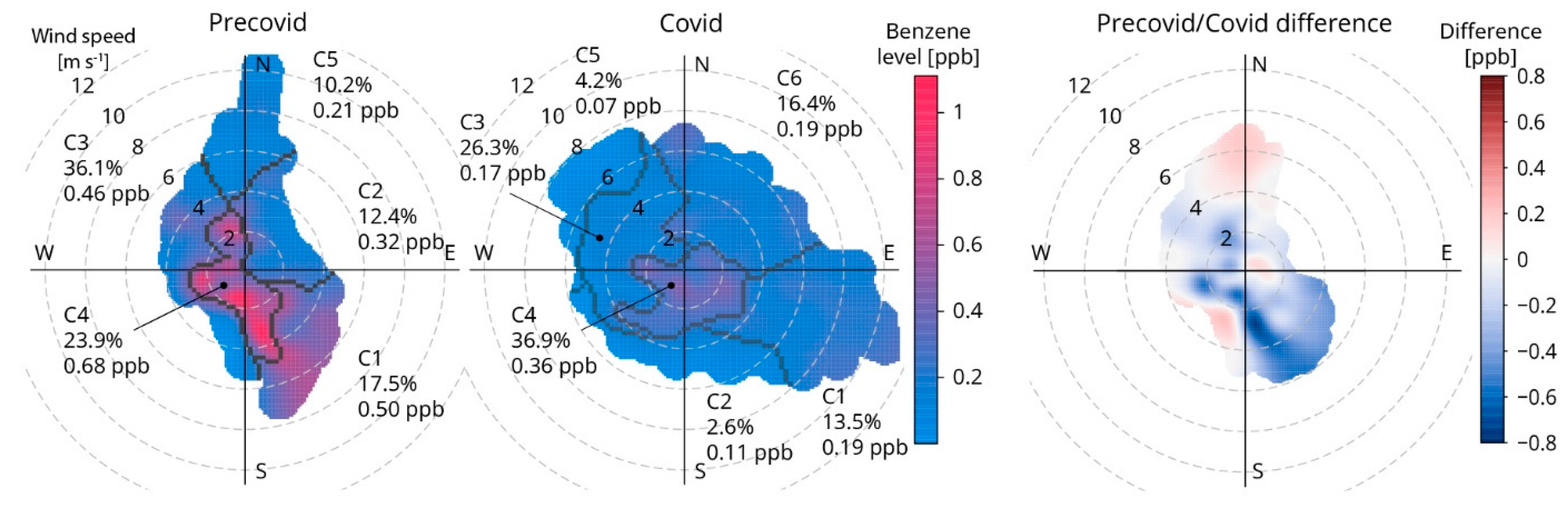
2.4.1. Bivariate Polar Plot

To identify potential spatial distribution of benzene emission sources, we employed a bivariate polar plot analysis [43] to examine the relationship between benzene concentrations and wind speed and direction. The analysis was conducted for periods before and during the state of emergency, with a focus on delineating differences in measured concentrations relative to wind characteristics, in order to assess the potential attenuation or intensification of specific sources and the emergence of new ones across different time frames. Subsequently, polar cluster analysis was applied to identify and group similar features and quantify the proportion of events associated with clusters.

2.4.2. Machine Learning

The data were analyzed using 7 regression tree ensemble machine learning algorithms that enhance prediction quality and robustness by combining multiple models into a single, more accurate model, and are particularly effective at reducing overfitting [44]. The ensembles include AdaBoost, ExtraTrees, Gradient Boosting, and Histogram Gradient Boosting (sklearn version 1.4), as well as CatBoost (1.2.7), LightGBM (4.5.0), and XGBoost (2.1.3). AdaBoost [45] increases focus on instances that were incorrectly predicted in previous rounds, thereby refining its performance continuously. CatBoost [46] optimizes gradient boosting by directly handling categorical features and reducing overfitting through ordered boosting. LightGBM [47] employs techniques like Gradient-based One-Side Sampling and Exclusive Feature Bundling to boost computational efficiency and feature management. XGBoost [48] constructs trees in parallel, supports multiple loss functions, and includes regularization to prevent overfitting. Both Gradient Boosting and Histogram Gradient Boosting, incorporated from the Python sklearn package [49], enhance modeling efficiency—Gradient Boosting builds models in a forward stage-wise fashion, while Histogram Gradient Boosting uses a binning method to speed up the training process and reduce memory usage.
To rigorously evaluate the performance of each model, we employed 5-fold cross-validation, ensuring comprehensive use of the dataset for both training and validation purposes, which significantly reduces the risk of overfitting. After training and evaluating the seven models, the top three performers were identified based on r-squared value and further refined to optimize performance using metaheuristics.

2.4.3. Metaheuristics

The effectiveness of machine learning models relies heavily on hyperparameter tuning, which is a nondeterministic polynomial-time (NP)-hard optimization challenge that is best addressed using metaheuristics. We incorporated six metaheuristic optimization algorithms to refine the hyperparameters of the top three models, thereby enhancing prediction accuracy. These algorithms included the Firefly Algorithm (FFA, [50]), Artificial Bee Colony (ABC, [51]), Harris Hawks Optimization (HHO, [52]), Sine Cosine Algorithm (SCA, [53]), Slime Mould Algorithm (SMA, [54]), and Quantum Search Algorithm (QSA, [55]) (mealpy version 3.0.1). These algorithms efficiently navigate the search space to identify near-optimal solutions. After determining the optimal hyperparameters for the three leading models, the best performing model was selected based on its r-squared value.

2.4.4. Explainable Artificial Intelligence

After identifying the best-performing model, we employed XAI methods SAGE and SHAP to ensure interpretability and transparency. SAGE assessed the global importance of each feature using an extension of the Shapley value from game theory, while SHAP values clarified each feature’s contribution to individual predictions, allowing for comprehensive analysis across the dataset to identify trends in feature contributions.
We also calculated relative and normalized SHAP values and introduced a categorical system for interpreting SHAP values, referred to as inherent SHAP values. Relative SHAP values denoted the proportion of absolute SHAP within the overall attributed significance of all features for a single prediction, reflecting the relative impact of each feature [10]. Normalized SHAP values, normalized to the expected value, simplified the understanding of impact magnitude [11]. For inherent SHAP values, high negative impacts were defined as those below the mean of all negative SHAP values. Moderate negative impacts ranged from this mean to −10% of the 95th percentile of all absolute SHAP values, while minor impacts spanned from −10% to 10% of this 95th percentile. Moderate positive impacts ranged from 10% of this percentile to the mean of positive SHAP values, and high positive impacts exceeded this mean. This classification system clarified the scale of each variable’s effect regardless of its absolute magnitude compared to other predictors and highlighted its distinct contributions to the model’s predictions. In this study, we utilized Python versions SAGE 0.2.4 and SHAP 0.46.0.

2.4.5. Cluster Analysis of Variable Impacts

To enhance the analytical depth of the study, we used dimensionality reduction and clustering techniques to analyze the relationships of variable local impacts. We utilized Uniform Manifold Approximation and Projection (UMAP, version 0.5.7, [56]) for dimensionality reduction, which preserves both local and global data structure, making it suitable for complex datasets. For clustering, we applied HDBSCAN [57] (version 0.8.40), which extends DBSCAN into a hierarchical clustering algorithm, dynamically selecting clusters based on data stability, allowing for the identification of clusters of varying densities. This combination allowed us to effectively identify and categorize localized impacts. Repeated framework executions consistently led to the identification of nine environmental settings, confirming the robustness of the clustering methodology.
According to the data and the obtained impacts, we have defined three ranges of normalized predictor levels: low (0–33%), medium (33–66%), and high (66–100%), for the variable absolute value, as well as three ranges of normalized impacts: low (1–5%), medium (5–15%), and high (15–100%).

3. Results and Discussion

3.1. Implementation of the State of Emergency

Prior to the state of emergency, benzene levels peaked at 2.26 ppb, with an average concentration of 0.48 ppb, driven by emission sources and weather conditions typical of the colder part of the year (Table S3, Supplementary Materials). In contrast, following the enactment of the emergency measures, the average benzene concentration was halved to 0.24 ppb, while peak levels dropped to 1.61 ppb.
Figure 1 visualizes the potential spatial distribution of benzene sources before and during the pandemic, enabling a direct comparison. The most intense sources, located in the N, NW, W, S, and SE, experienced significant reductions or were deactivated following the emergency measures. In the S and E areas, observed concentrations decreased by up to 0.8 ppb. However, new emission sources emerged in the N and SW areas.
The March state of emergency significantly impacted air quality, primarily driven by movement restrictions, institutional closures, reduced industrial activity, and decreased traffic. These combined factors led to more stable benzene levels with smaller variations. Despite the sampling site being influenced by light to fresh breeze winds (2 to 10 m s−1) from the north and east, regions typically associated with intense anthropogenic activities, no significant contribution to benzene concentrations was observed from these areas, likely due to the imposed governmental measures and subsequent changes in human behavior (Figure 2). Additionally, the onset of the state of emergency coincided with the transition into the warmer part of the year, suggesting that seasonal atmospheric changes and meteorological factors also contributed to the observed decrease in benzene concentrations. While lockdown measures were a dominant factor, the role of seasonal and meteorological variability cannot be overlooked. Future research will further refine this assessment by explicitly accounting for seasonal influences in a more comprehensive environmental analysis.

3.2. Modelling Results

The global explanation of the best-performing model (Gradient boosting model optimized with SCA metaheuristics, with MAE 0.034, max error 0.34, MSE 0.003, RMSE 0.056, MAPE 0.168, and R2 0.94—MAE improvement of 15.1% compared to the non-optimized model) using SAGE revealed that 81 out of the 404 analyzed variables accounted for 95% of the global impact for benzene level prediction during the state of emergency (Table S4, Supplementary Materials). Notably, only 15 variables emerged as having a global impact greater than 1% (in descending order: m129, m41, m105, m97, m42, m45, m107, m95, m135, m62, m133, PM10, m93, m163, and m73). Utilizing our clustering approach with SHAP explanations, we identified nine distinct groups of variable impacts, each representing a specific environmental setting (E0–E8). This method sheds light on how key factors sculpt the environmental context that affects benzene concentrations, particularly in emergency situations, like a pandemic, where changes in human activities play a significant role (Table 1). Additionally, a tenth group, E-1, remained unclustered, encompassing data instances likely to represent outliers or transitional regimes, rendering them unsuitable for categorization within a specific environmental setting.
The majority of data instances were grouped into E1 (38.6%), followed by E3 (10.5%), E7 (7.2%), and E6 (6.5%). The five least represented environmental settings accounted for 2.9% to 5.8% of the data, reflecting isolated or periodic events rather than consistent environmental regimes. Notably, three of these settings were associated with an increase in benzene levels relative to the expected value: E7 (0.37 ppb in average), E5 (0.26 ppb), and E2 (0.02 ppb). In contrast, the remaining settings demonstrated negative mean impacts from −0.12 to −0.01 ppb, indicating that the combinations of variables in these contexts are linked to environments characterized by lower benzene concentrations.
Based on the distribution of normalized variable levels and impacts across environmental settings (Figure 3), 27 variables, each with varying roles and magnitudes, are associated with the environmental fate of benzene. These include 18 VOCs (m41, m42, m45, m47, m62, m73, m75, m93, m95, m135, m61, m97, m105, m107, m129, m130, m133, and m163), two criteria air pollutants (PM10 and CO), three meteorological variables (total cloud cover—tcld, best four-layer lifted index—lib4, and temperature at 2 m—t02m), and four pandemic variables (confirmed deaths, total active cases lag 1, confirmed cases lag 2, and parks percentage change lag 3). Notably, m41, m42, m105, and m129 emerge as key determinants across all settings. We acknowledge that the ion signals at these masses could correspond to a variety of compounds. For instance, m41 could be associated with alcohols, such as propanol, butanol, pentanol, and octanol, isoprene, acetonitrile, as well as 1-octen-3-ol and naphthalene—both identified at m129 (Table S1, Supplementary Materials). However, based on existing literature, we believe that the most likely compound at m41 is propyne. Similarly, the signals at m42, m105, and m129 are most likely attributable to acetonitrile, styrene, and naphthalene, respectively.
Among the most influential variables, m45 (acetaldehyde) and m97 (cycloheptene) are key factors in nearly every environmental setting, with m107 (C8 aromatics) impacting all but two. Meanwhile, lib4, m62 (vinyl chloride), m95 (phenol or dimethyl sulfide), and m135 (C10 aromatics) play significant roles in all but three settings (Figure 3). The remaining variables offer valuable insights that can help trace the origins of benzene within each specific context, with special attention given to those that describe or reflect the immediate or delayed changes in human activities in response to the pandemic.
The environmental setting E3 initially aligned with the introduction of the state of emergency (Figure 4) while, as time progressed, the tightening of restrictions gave rise to periodic events attributed to E7 and regime E6. The subsequent relaxation of measures triggered the onset of environmental setting E1. The remaining settings represent isolated benzene pollution events that coincided with the development of specific environmental conditions. For the purpose of this study, we will focus on analyzing three environmental settings that marked the onset of the state of emergency: E3, E4, and E7.

3.2.1. Environmental Setting E3—Chemical Manufacturing, Combustion, and Petroleum-Related Emissions

During the first week of the state of emergency, the environmental setting identified as E3 became prominent, accounting for 10.5% of the total data instances (Figure 4). In this environmental content, observed benzene levels were, on average, 15.7% lower than the expected value (0.244 ppb; Table 1).
The setting was primarily driven by 12 key variables, including a combination of VOCs, temperature (t02m), and lib4. As shown in Figure 5, the principal contributors among these were VOCs identified as cycloheptene, acetonitrile, styrene, and naphthalene, with relative impacts of 11.0%, −7.0%, −7.9%, and −11.9%, respectively, and medium mean normalized impacts on benzene level prediction of 8.5%, −5.2%, −6.0%, and −8.9% (Tables S1 and S5, Supplementary Materials). These compounds originate from petroleum refining, industrial emissions, chemical and plastic manufacturing, as well as the combustion of biomass, fossil fuels (vehicle exhaust, residential heating), coal, and wood [58,59], activities that are prevalent in the facilities surrounding the sampling site.
The positive association between benzene and cycloheptene (Group 1) suggests common sources that elevate benzene concentrations. In contrast, the negative association with styrene, and acetonitrile (Group 2), and even stronger negative association with naphthalene (Group 3), indicate that these compounds share sources that contribute to a reduction in benzene concentrations, with the sources of naphthalene likely being the weakest or most diminished among them. Industrial processes, including petroleum refining, storage and distribution, the production of synthetic rubber and plastics, and various combustion activities, like vehicle exhaust and biomass burning, are common sources of both cycloheptene and benzene. However, these processes are not necessarily associated with other compounds in Groups 2 and 3. The E3 setting was characterized by light to fresh breeze winds (averaging 5 m s−1) from the north and especially the east, where the Pančevo Oil Refinery is located. Despite these conditions, the high levels of lib4 (averaging 12.5 °C) with minimal impact on benzene prediction indicate an atmosphere with significant vertical and some horizontal stability. This is likely to have limited vertical mixing, causing pollutants to remain near the surface. The wind speed was insufficient to disperse these pollutants effectively over a wide area, suggesting that the influence of distant sources, including the refinery, was insignificant, though other petroleum-related activities near the sampling site might still have been relevant. Given that the heating season was ongoing during the E3 period, local sources, particularly biomass burning for residential heating, are likely to have contributed to the observed increase in benzene concentrations. This is further supported by the observation that naphthalene levels and impacts were higher at night, as the extended time spent at home due to restrictions prolonged the heating period into the evening hours.
In the case of Group 2, chemical manufacturing, particularly the production of acrylonitrile and polystyrene, emerged as a significant source, and the reduction in emissions from these activities ultimately led to a decrease in benzene levels. Regarding Group 3, the negative impact of naphthalene on benzene predictions, which is a byproduct of incomplete combustion of gasoline and diesel [60], was likely to have been attributable to reduced traffic activity near the measurement site. The onset of the state of emergency, coinciding with the first registered COVID-19 cases, resulted in the closure of numerous institutions and schools, thereby significantly reducing vehicle usage. This reduction in traffic not only decreased emissions of key pollutants but also led to a lower presence of nitrogen oxides (NOx), which are precursors to both ozone and benzene formation. The primary compounds that contribute to benzene levels, including its precursors, are known to react with hydroxyl radicals, nitrate radicals and ozone, which leads to the formation of secondary pollutants, such as acetaldehyde. The observed further reductions in benzene levels appear to be linked to increased ozone concentrations, a phenomenon attributed to the reduction of aerosol and nitrogen oxide concentrations during the restrictions [61].
Finally, considering the other VOCs associated with this setting, their low levels resulted in low negative impacts on benzene prediction for propyne, acetaldehyde, C8 aromatics, phenol, dimethyl sulfide, vinyl chloride, and toluene (m93). This limited impact, coupled with the low concentrations, suggests a significant reduction in emissions from their typical sources.
At the end of the first week of the state of emergency, as the weekend began, benzene concentration patterns were influenced by the emergence of two additional environmental settings, E7 and E4 (Figure 4). Occurrences of E3 reappeared only in the middle of the second week of the state of emergency, but this setting faded before the second weekend, coinciding with the first implementation of the curfew.

3.2.2. Environmental Setting E7—Non-Combustion Emissions, Nocturnal Chemistry, and Meteorological Context

Within the environmental setting E7, which accounted for 7.2% of the data instances, benzene levels were notably elevated, with an average of 0.37 ppb. This setting captured high benzene events that periodically occurred and persisted until the final curfew, primarily during nighttime and early morning hours (10 p.m.–8 a.m.) towards the end of the workweek.
Benzene levels in this setting varied significantly, ranging from −8% to 421% relative to the expected value. These fluctuations were largely driven by 19 variables, including a mix of VOCs, CO, PM10, and meteorological parameters (Figure 5). The most influential variables in predicting benzene levels were naphthalene (relative impact 21.4%), cycloheptene (7.8%), propyne (5.2%), and phenol/dimethyl sulfide (4.0%), contributing to increases of 50%, 14%, 13%, and 12%, respectively (Table S6, Supplementary Materials). Overall, the variables contributed highly positively to the prediction of benzene levels, except for C10 aromatics and lib4, which had moderate positive impacts, and styrene (m105), with a minor impact.
Among the compounds observed at high levels, naphthalene was the only one that made a significant contribution to the prediction of benzene levels, while cycloheptene and acetonitrile had moderate impacts, and CO had a minor impact (Table S6). These compounds reflect a mix of emissions from industrial activities and fossil fuels, as previously discussed, as well as potential nocturnal chemistry under specific atmospheric conditions [62]. This interpretation aligns with our findings, as the levels and corresponding impacts of styrene, cycloheptene, acetonitrile, PM10, and CO increased during nighttime. In urban atmospheres, significant amounts of NO are oxidized to NO2, which is then converted to the nitrate radical (NO3) by ozone. NO3, the primary nocturnal tropospheric oxidant, accumulates at night due to its rapid degradation through photolysis and reaction with NO during daylight. At night, NO3-driven reactions significantly influence air pollution and regulate the lifespan of various trace gases, including VOCs, leading to the formation of complex oxidation products. The high concentration and reactivity of NO3 make it responsible for the degradation of many unsaturated hydrocarbons during the night. For instance, styrene concentrations increased significantly within the stable nocturnal boundary layer, resulting in heightened reactivity. Styrene thus serves as an effective indicator of NO3 reactivity across different seasons and for estimating NO3 reactivity toward other VOCs [62]. Conversely, the opposite trend was observed for propyne, C8 aromatics, C10 aromatics, fragmentation ions at m133, and lib4 (Table S6, Supplementary Materials).
Among the compounds exhibiting medium levels, propyne, styrene, acetaldehyde, and phenol/dimethyl sulfide recorded medium, while C8 aromatics, C10 aromatics, vinyl chloride, fragmentation ions at m133, PM10, C12 aromatics, and hydroxy acetone showed low impacts on benzene prediction. The relatively low impacts of CO and PM10 suggested that combustion played a lesser role in this setting compared to other potential sources of benzene, a conclusion further supported by the periodic nature of this setting. Additionally, the analysis of traffic intensity during the weekdays revealed no surge in activity prior to curfews, making it unlikely that vehicle exhaust significantly contributed to the observed benzene levels.
The strong association of benzene and naphthalene, with their concentration consistently increasing during the workweek, then declining over the weekend, likely originating from non-combustion processes. These joint emissions can be attributed to various nearby facilities, including an oil refinery (NE and E), textile recycling (E and SE), paper industry (NW, W, SW, S, and SE), rubber and plastic production (W, NW, S, SE, E, and N), and furniture manufacturing (W, SW, S, SE, and E). The levels and impacts of VOCs generally decreased as the duration of this setting progressed, aligning with the reduction in anthropogenic activities due to increasing restrictions. Moreover, typical human activities intensified before each weekend curfew as people prepared for the impending lockdown, likely affecting the observed environmental conditions.
The meteorological context, shaped by the best four-layer lifted index, temperature, and total cloud cover, played an important role in defining this setting. Calm to light breeze winds (0–3.3 m s−1) and medium levels of lib4, which exhibited a low impact on benzene prediction, suggest that, although dispersion and transport processes were present, they did not significantly affect benzene concentrations. While the observed medium-level temperatures (up to 13 °C) are likely to have accelerated chemical reactions, potentially increasing secondary pollutants like ozone and particulate matter [63], the nocturnal nature of this setting suggests that ozone formation was minimal during the early morning hours. Additionally, our results indicate that the recorded temperature levels had only a modest impact on benzene dynamics, averaging 1.3%.
Low levels of total cloud cover (tcld) had a low but notable positive impact on benzene levels through various mechanisms. At night, cloud cover traps pollutants closer to the surface by reducing the radiative cooling and preventing rapid heat loss, stabilizing the lower atmosphere and leading to pollutant accumulation near the ground [64]. During the day, tcld plays a critical role in modulating solar radiation, potentially lowering surface temperatures, which might reduce the volatilization rate of some VOCs or slow down the photochemical reactions necessary for the formation of certain secondary pollutants. The higher positive impact observed during the day compared to night suggests that cloud cover plays a more crucial role in shaping benzene prediction during daylight hours in this environmental setting.

3.2.3. Environmental Setting E4—Local Industrial Processes

Setting E4, accounting for 5.4% of data instances, emerged during the first weekend of the state of emergency and persisted until the following weekend as an isolated event (Figure 4). It contributed to a slight further reduction in observed benzene levels, averaging 2.33% below the expected value (Table 1).
The setting was primarily driven by eight variables, including a combination of VOCs and lib4 (Figure 5). The key contributors were cycloheptene (5.0%), naphthalene (−3.3%), acetonitrile (−3.4%), and styrene (−8.3%), with mean normalized impacts on benzene prediction of 4.4%, −1.1%, −2.4%, and −6.2%, respectively (Table S7, Supplementary Materials).
The differentiation between cycloheptene and benzene (Group 1), naphthalene, acetonitrile, and benzene (Group 2), and styrene and benzene (Group 3) primarily arises from specific industrial activities and combustion processes. Although Groups 1 and 2 share common sources, such as vehicle exhaust and industrial emissions, Group 2 is more specifically associated with chemical production activities, which play a less prominent role in the origin of the Group 1 compounds. Group 1 is closely associated with combustion processes, like vehicle exhaust, residential heating, and biomass burning, as well as industrial emissions from petroleum refining. Reduced commuting and increased time spent at home due to restrictive measures intensified emissions from residential heating and biomass burning. In contrast, Group 2 is more associated with chemical manufacturing processes and coal tar processing where acetonitrile and naphthalene are produced alongside benzene. Group 3 is distinct for its strong ties to plastic and resin production, where styrene is a key component, and its presence alongside benzene highlights these specific industrial activities. The light to moderate breeze (1.5–6 m s−1) from the N and NW within this setting carried cleaner air from regions where the sources of Group 2 and 3 emissions were located, which were already operating at reduced capacity due to the state of emergency, further diminishing their impact and leading to benzene concentrations lower than those expected.
Similar to the E3, high levels of lib4 (mean 10.1 °C), which resulted in low impacts on benzene prediction suggest a stable atmosphere both vertically and, to some extent, horizontally. This stability is likely to have limited vertical mixing, with stratified air masses keeping pollutants close to the surface, thereby reducing the impact of more distant industrial facilities.

4. Conclusions

This study introduced a novel approach centered on “environmental settings”, the combination of natural and human factors that govern air pollutant behavior. By integrating pollutant concentrations with contextual variables (e.g., meteorological conditions, temporal factors, and human activities), our AI framework offers a comprehensive view of benzene dynamics, surpassing the limitations of traditional source apportionment techniques.
Our methodology, combining advanced machine learning, metaheuristic optimization, explainable AI, and clustering, identified key drivers of benzene concentrations. Techniques like bivariate polar plots, polar clustering, SAGE, and SHAP uncovered both spatial patterns and model insights across diverse environmental settings. Applied to Belgrade’s benzene data during the onset of COVID-19, the approach revealed how severely reduced transportation and industrial activities only modestly lowered benzene levels. This finding highlights the importance of considering a broad range of factors beyond direct emissions.
Overall, this framework provides actionable knowledge for air quality management, demonstrating how “environmental settings” can inform crisis responses and routine policies alike. By quantifying the maximum possible impact of altered activities and processes, decision-makers can better anticipate and mitigate changes in pollution levels. While a formal sensitivity analysis was not conducted, the stability of the results across iterations suggests that the selected number of clusters is representative. Future research will further refine this framework by incorporating an extended set of predictors to enhance environmental setting characterization. Additionally, future research will focus on uncertainty propagation and on assessing the stability of predictor importance rankings across multiple model runs, and providing confidence intervals to ensure greater robustness and reliability of the results.

Supplementary Materials

The following supporting information can be downloaded at: https://www.mdpi.com/article/10.3390/atmos16020231/s1, Figure S1: Location of the study area in Belgrade and a photograph of the monitoring site (Source: Google Maps); Figure S2: Normalized sensitivities and the relative transmission curve; Table S1: Compounds detected by PTR-MS in ambient air; Table S2: Global data assimilation system data abbreviations; Table S3: Descriptive statistics for measured parameters before and after the introduction of the state of emergency; Table S4: SAGE statistics; Table S5: Environmental setting E3 statistics; Table S6: Environmental setting E7 statistics; Table S7: Environmental setting E4 statistics.

Author Contributions

N.R.: Funding acquisition, Investigation. M.P.: Conceptualization, Data Curation, Formal Analysis, Funding acquisition, Investigation, Writing—original draft, Writing—review and editing. G.J.: Conceptualization, Formal Analysis, Funding acquisition, Investigation, Writing—original draft, Writing—review and editing. T.B.: Methodology, Project Administration, Resources, Software. S.S.: Funding acquisition, Investigation, Writing—original draft, Writing—review and editing. N.S.: Data curation. A.S.: Conceptualization, Data Curation, Formal Analysis, Funding acquisition, Investigation, Methodology, Project Administration, Resources, Software, Supervision, Validation, Visualization, Writing—original draft, Writing—review and editing. All authors have read and agreed to the published version of the manuscript.

Funding

The authors acknowledge funding provided by the Institute of Physics Belgrade, through a grant by the Ministry of Education, Science and Technological Development of the Republic of Serbia, as well as by the Science Fund of the Republic of Serbia, Grant No. #7373, Characterizing crises-caused air pollution alternations using an artificial intelligence-based framework—crAIRsis.

Institutional Review Board Statement

Not applicable.

Informed Consent Statement

Not applicable.

Data Availability Statement

The original contributions presented in this study are included in the article. Further inquiries can be directed to the corresponding author(s).

Conflicts of Interest

The authors declare no conflict of interest.

References

  1. Zahed, M.A.; Salehi, S.; Khoei, M.A.; Esmaeili, P.; Mohajeri, L. Risk assessment of Benzene, Toluene, Ethyl benzene, and Xylene (BTEX) in the atmospheric air around the world: A review. Toxicol. Vitr. 2024, 98, 105825. [Google Scholar] [CrossRef]
  2. Li, D.; Tao, X.; Song, X.; Liu, S.; Yuan, K.; Deng, F.; Guo, Y. Ambient volatile organic compounds concentration variation characteristics and source apportionment in Lanzhou, China during the COVID-19 lockdown. Atmos. Pollut. Res. 2024, 15, 102064. [Google Scholar] [CrossRef]
  3. Cardito, A.; Carotenuto, M.; Amoruso, A.; Libralato, G.; Lofrano, G. Air quality trends and implications pre and post COVID-19 restrictions. Sci. Total Environ. 2023, 879, 162833. [Google Scholar] [CrossRef] [PubMed]
  4. Ling, C.; Cui, L.; Li, R. Global impact of the COVID-19 lockdown on surface concentration and health risk of atmospheric benzene. Atmos. Chem. Phys. 2023, 23, 3311–3324. [Google Scholar] [CrossRef]
  5. Covert, I.; Lundberg, S.M.; Lee, S.I. Understanding global feature contributions with additive importance measures. Adv. Neural Inf. Process. Syst. 2020, 33, 17212–17223. [Google Scholar]
  6. Lundberg, S. A unified approach to interpreting model predictions. arXiv 2017, arXiv:1705.07874. [Google Scholar]
  7. Bacanin, N.; Perisic, M.; Jovanovic, G.; Damaševičius, R.; Stanisic, S.; Simic, V.; Zivkovic, M.; Stojic, A. The explainable potential of coupling hybridized metaheuristics, XGBoost, and SHAP in revealing toluene behavior in the atmosphere. Sci. Total Environ. 2024, 929, 172195. [Google Scholar] [CrossRef] [PubMed]
  8. Jovanovic, G.; Perisic, M.; Bacanin, N.; Zivkovic, M.; Stanisic, S.; Strumberger, I.; Alimpic, F.; Stojic, A. Potential of coupling metaheuristics-optimized-XGBoost and SHAP in revealing PAHs environmental fate. Toxics 2023, 11, 394. [Google Scholar] [CrossRef] [PubMed]
  9. Jovanovic, L.; Jovanovic, G.; Perisic, M.; Alimpic, F.; Stanisic, S.; Bacanin, N.; Zivkovic, M.; Stojic, A. The explainable potential of coupling metaheuristics-optimized-xgboost and shap in revealing vocs’ environmental fate. Atmosphere 2023, 14, 109. [Google Scholar] [CrossRef]
  10. Stojić, A.; Jovanović, G.; Stanišić, S.; Romanić, S.H.; Šoštarić, A.; Udovičić, V.; Perišić, M.; Milićević, T. The PM2. 5-bound polycyclic aromatic hydrocarbon behavior in indoor and outdoor environments, part II: Explainable prediction of benzo [a] pyrene levels. Chemosphere 2022, 289, 133154. [Google Scholar] [CrossRef] [PubMed]
  11. Jovanović, G.; Perišić, M.; Bezdan, T.; Stanišić, S.; Radusin, K.; Popović, A.; Stojić, A. The PM 2.5-Bound Polycyclic Aromatic Hydrocarbon Behavior in Indoor and Outdoor Environments, Part III: Role of Environmental Settings in Elevating Indoor Concentrations of Benzo (a) pyrene. Atmosphere 2024, 15, 1520. [Google Scholar] [CrossRef]
  12. Government of Serbia. 2020. Available online: https://www.srbija.gov.rs/vest/en/155727/serbia-lifts-state-of-emergency.php (accessed on 1 June 2023).
  13. Lindinger, W.; Hansel, A.; Jordan, A. On-line monitoring of volatile organic compounds at pptv levels by means of proton-transfer-reaction mass spectrometry (PTR-MS) medical applications, food control and environmental research. Int. J. Mass Spectrom. Ion Processes 1998, 173, 191–241. [Google Scholar] [CrossRef]
  14. Stojić, A.; Maletić, D.; Stojić, S.S.; Mijić, Z.; Šoštarić, A. Forecasting of VOC emissions from traffic and industry using classification and regression multivariate methods. Sci. Total Environ. 2015, 521, 19–26. [Google Scholar] [CrossRef] [PubMed]
  15. Taipale, R.; Ruuskanen, T.M.; Rinne, J.; Kajos, M.K.; Hakola, H.; Pohja, T.; Kulmala, M. Quantitative long-term measurements of VOC concentrations by PTR-MS–measurement, calibration, and volume mixing ratio calculation methods. Atmos. Chem. Phys. 2008, 8, 6681–6698. [Google Scholar] [CrossRef]
  16. Blake, R.S.; Monks, P.S.; Ellis, A.M. Proton-transfer reaction mass spectrometry. Chem. Rev. 2009, 109, 861–896. [Google Scholar] [CrossRef] [PubMed]
  17. Buhr, K.; van Ruth, S.; Delahunty, C. Analysis of volatile flavour compounds by Proton Transfer Reaction-Mass Spectrometry: Fragmentation patterns and discrimination between isobaric and isomeric compounds. Int. J. Mass Spectrom. 2002, 221, 1–7. [Google Scholar] [CrossRef]
  18. Dunne, E.; Galbally, I.E.; Lawson, S.; Patti, A. Interference in the PTR-MS measurement of acetonitrile at m/z 42 in polluted urban air—A study using switchable reagent ion PTR-MS. Int. J. Mass Spectrom. 2012, 319, 40–47. [Google Scholar] [CrossRef]
  19. Zannoni, N.; Gros, V.; Lanza, M.; Sarda, R.; Bonsang, B.; Kalogridis, C.; Preunkert, S.; Legrand, M.; Jambert, C.; Boissard, C.; et al. OH reactivity and concentrations of biogenic volatile organic compounds in a Mediterranean forest of downy oak trees. Atmos. Chem. Phys. 2016, 16, 1619–1636. [Google Scholar] [CrossRef]
  20. Nakajima, S.; Asakawa, T.; Sekiguchi, O.; Tajima, S.; Nibbering, N.M. The formation of protonated dimethyl ether from the metastable molecular ions of 1-methoxy-2-propanol, CH3OCH2CH (OH) CH3. Eur. J. Mass Spectrom. 2001, 7, 47–53. [Google Scholar] [CrossRef]
  21. Wang, R.; Zhang, Y.; Jiao, L.; Zhao, X.; Gao, Z.; Dong, D. Proton-Transfer-Reaction Mass Spectrometry for Rapid Dynamic Measurement of Ethylene Oxide Volatilization from Medical Masks. Atmosphere 2024, 15, 114. [Google Scholar] [CrossRef]
  22. Brown, P.; Watts, P.; Märk, T.D.; Mayhew, C.A. Proton transfer reaction mass spectrometry investigations on the effects of reduced electric field and reagent ion internal energy on product ion branching ratios for a series of saturated alcohols. Int. J. Mass Spectrom. 2010, 294, 103–111. [Google Scholar] [CrossRef]
  23. Baasandorj, M.; Millet, D.B.; Hu, L.; Mitroo, D.; Williams, B.J. Measuring acetic and formic acid by proton-transfer-reaction mass spectrometry: Sensitivity, humidity dependence, and quantifying interferences. Atmos. Meas. Tech. 2015, 8, 1303–1321. [Google Scholar] [CrossRef]
  24. Inomata, S.; Tanimoto, H.; Kato, S.; Suthawaree, J.; Kanaya, Y.; Pochanart, P.; Liu, Y.; Wang, Z. PTR-MS measurements of non-methane volatile organic compounds during an intensive field campaign at the summit of Mount Tai, China, in June 2006. Atmos. Chem. Phys. 2010, 10, 7085–7099. [Google Scholar] [CrossRef]
  25. Pal, P.; Banat, F. Comparison of thermal degradation between fresh and industrial aqueous methyldiethanolamine with continuous injection of H2S/CO2 in high pressure reactor. J. Nat. Gas Sci. Eng. 2016, 29, 479–487. [Google Scholar] [CrossRef]
  26. Awasthi, A.; Sinha, B.; Hakkim, H.; Mishra, S.; Mummidivarapu, V.; Singh, G.; Ghude, S.D.; Soni, V.K.; Nigam, N.; Sinha, V.; et al. Biomass burning sources control ambient particulate matter but traffic and industrial sources control VOCs and secondary pollutant formation during extreme pollution events in Delhi. EGUsphere 2024, 1–35. [Google Scholar] [CrossRef]
  27. Van Huffela, K.; Hansenb, M.J.; Feilbergb, A.; Liub, D.; Van Langenhovea, H. The power of online proton transfer reaction-mass spectrometry (PTR-MS) measurement of odorous emissions from a pig house. Chem. Eng. 2014, 40, 241–246. [Google Scholar]
  28. Chen, L.; Yan, R.; Zhao, Y.; Sun, J.; Zhang, Y.; Li, H.; Zhao, D.; Wang, B.; Ye, X.; Sun, B. Characterization of the aroma release from retronasal cavity and flavor perception during baijiu consumption by Vocus-PTR-MS, GC× GC-MS, and TCATA analysis. LWT 2023, 174, 114430. [Google Scholar] [CrossRef]
  29. De Gouw, J.; Warneke, C. Measurements of volatile organic compounds in the earth’s atmosphere using proton-transfer-reaction mass spectrometry. Mass Spectrom. Rev. 2007, 26, 223–257. [Google Scholar] [CrossRef] [PubMed]
  30. Perraud, V.; Meinardi, S.; Blake, D.R.; Finlayson-Pitts, B.J. Challenges associated with the sampling and analysis of organosulfur compounds in air using real-time PTR-ToF-MS and offline GC-FID. Atmos. Meas. Tech. 2016, 9, 1325–1340. [Google Scholar] [CrossRef]
  31. Papurello, D.; Silvestri, S.; Tomasi, L.; Belcari, I.; Biasioli, F.; Santarelli, M. Natural gas trace compounds analysis with innovative systems: PTR-ToF-MS and FASTGC. Energy Procedia 2016, 101, 536–541. [Google Scholar] [CrossRef]
  32. Mallette, N.D.; Knighton, W.B.; Strobel, G.A.; Carlson, R.P.; Peyton, B.M. Resolution of volatile fuel compound profiles from Ascocoryne sarcoides: A comparison by proton transfer reaction-mass spectrometry and solid phase microextraction gas chromatography-mass spectrometry. AMB Express 2012, 2, 1–13. [Google Scholar] [CrossRef] [PubMed]
  33. Tasin, M.; Cappellin, L.; Biasioli, F. Fast direct injection mass-spectrometric characterization of stimuli for insect electrophysiology by proton transfer reaction-time of flight mass-spectrometry (PTR-ToF-MS). Sensors 2012, 12, 4091–4104. [Google Scholar] [CrossRef]
  34. Bruns, E.A.; Slowik, J.G.; El Haddad, I.; Kilic, D.; Klein, F.; Dommen, J.; Temime-Roussel, B.; Marchand, N.; Baltensperger, U.; Prévôt, A.S. Characterization of gas-phase organics using proton transfer reaction time-of-flight mass spectrometry: Fresh and aged residential wood combustion emissions. Atmos. Chem. Phys. 2017, 17, 705–720. [Google Scholar] [CrossRef]
  35. Westphal, F.; Junge, T. Ring positional differentiation of isomeric N-alkylated fluorocathinones by gas chromatography/tandem mass spectrometry. Forensic Sci. Int. 2012, 223, 97–105. [Google Scholar] [CrossRef]
  36. Erickson, M.H.; Gueneron, M.; Jobson, B.T. Measuring long chain alkanes in diesel engine exhaust by thermal desorption PTR-MS. Atmos. Meas. Tech. Discuss. 2013, 6, 6005–6046. [Google Scholar] [CrossRef]
  37. SEPA. 2022. Available online: http://amskv.sepa.gov.rs/mob/index.php?lng=en (accessed on 1 June 2023).
  38. GDAS. 2022. Available online: https://www.ncei.noaa.gov/access/metadata/landing-page/bin/iso?id=gov.noaa.ncdc:C00379 (accessed on 1 June 2023).
  39. Oxford COVID-19 Government Response Tracker. OxCovid19 Database. 2022. Available online: https://covid19.oii.ox.ac.uk/database/ (accessed on 1 June 2023).
  40. Worldometer. COVID-19 Coronavirus Pandemic Data [Data Set]. 2022. Available online: https://www.worldometers.info/coronavirus/ (accessed on 1 June 2023).
  41. Apple Inc. COVID-19—Mobility Trends Reports. 2022. Available online: https://www.apple.com/covid19/mobility (accessed on 1 June 2023).
  42. Google LLC. COVID-19 Community Mobility Reports. 2022. Available online: https://www.google.com/covid19/mobility/ (accessed on 1 June 2023).
  43. Carslaw, D.C.; Beevers, S.D. Characterising and understanding emission sources using bivariate polar plots and k-means clustering. Environ. Model. Softw. 2013, 40, 325–329. [Google Scholar] [CrossRef]
  44. Dietterich, T.G. Ensemble methods in machine learning. In International Workshop on Multiple Classifier Systems; Springer: Berlin/Heidelberg, Germany, 2000; pp. 1–15. [Google Scholar]
  45. Freund, Y.; Schapire, R.E. A decision-theoretic generalization of on-line learning and an application to boosting. J. Comput. Syst. Sci. 1997, 55, 119–139. [Google Scholar] [CrossRef]
  46. Prokhorenkova, L.; Gusev, G.; Vorobev, A.; Dorogush, A.V.; Gulin, A. CatBoost: Unbiased boosting with categorical features. Adv. Neural Inf. Process. Syst. 2018, 31. Available online: https://proceedings.neurips.cc/paper/2018/hash/14491b756b3a51daac41c24863285549-Abstract.html (accessed on 12 December 2024).
  47. Ke, G.; Meng, Q.; Finley, T.; Wang, T.; Chen, W.; Ma, W.; Ye, Q.; Liu, T.Y. Lightgbm: A highly efficient gradient boosting decision tree. Adv. Neural Inf. Process. Syst. 2017, 30. Available online: https://proceedings.neurips.cc/paper/2017/hash/6449f44a102fde848669bdd9eb6b76fa-Abstract.html (accessed on 12 December 2024).
  48. Friedman, J.H. Greedy function approximation: A gradient boosting machine. Ann. Stat. 2001, 29, 1189–1232. [Google Scholar] [CrossRef]
  49. Pedregosa, F.; Varoquaux, G.; Gramfort, A.; Michel, V.; Thirion, B.; Grisel, O.; Blondel, M.; Prettenhofer, P.; Weiss, R.; Dubourg, V.; et al. Scikit-learn: Machine learning in Python. J. Mach. Learn. Res. 2011, 12, 2825–2830. [Google Scholar]
  50. Yang, X.S. Firefly algorithms for multimodal optimization. In International Symposium on Stochastic Algorithms; Springer: Berlin/Heidelberg, Germany, 2009; pp. 169–178. [Google Scholar]
  51. Karaboga, D. An Idea Based on Honey Bee Swarm for Numerical Optimization; Technical Report-tr06; Computer Engineering Department, Engineering Faculty, Erciyes University: Kayseri, Turkey, 2005; Volume 200, pp. 1–10. [Google Scholar]
  52. Heidari, A.A.; Mirjalili, S.; Faris, H.; Aljarah, I.; Mafarja, M.; Chen, H. Harris hawks optimization: Algorithm and applications. Future Gener. Comput. Syst. 2019, 97, 849–872. [Google Scholar] [CrossRef]
  53. Mirjalili, S. SCA: A sine cosine algorithm for solving optimization problems. Knowl.-Based Syst. 2016, 96, 120–133. [Google Scholar] [CrossRef]
  54. Li, S.; Chen, H.; Wang, M.; Heidari, A.A.; Mirjalili, S. Slime mould algorithm: A new method for stochastic optimization. Future Gener. Comput. Syst. 2020, 111, 300–323. [Google Scholar] [CrossRef]
  55. Zhang, J.; Xiao, M.; Gao, L.; Pan, Q. Queuing search algorithm: A novel metaheuristic algorithm for solving engineering optimization problems. Appl. Math. Model. 2018, 63, 464–490. [Google Scholar] [CrossRef]
  56. McInnes, L.; Healy, J.; Melville, J. Umap: Uniform manifold approximation and projection for dimension reduction. arXiv 2018, arXiv:1802.03426. [Google Scholar]
  57. McInnes, L.; Healy, J.; Astels, S. hdbscan: Hierarchical density-based clustering. J. Open Source Softw. 2017, 2, 205. [Google Scholar] [CrossRef]
  58. Kong, L.; Zhou, L.; Chen, D.; Luo, L.; Xiao, K.; Chen, Y.; Liu, H.; Tan, Q.; Yang, F. Atmospheric oxidation capacity and secondary pollutant formation potentials based on photochemical loss of VOCs in a megacity of the Sichuan Basin, China. Sci. Total Environ. 2023, 901, 166259. [Google Scholar] [CrossRef] [PubMed]
  59. Zhang, L.; Xu, T.; Wu, G.; Zhang, C.; Li, Y.; Wang, H.; Gong, D.; Li, Q.; Wang, B. Photochemical loss with consequential underestimation in active VOCs and corresponding secondary pollutions in a petrochemical refinery, China. Sci. Total Environ. 2024, 918, 170613. [Google Scholar] [CrossRef]
  60. Marques, B.; Kostenidou, E.; Valiente, A.M.; Vansevenant, B.; Sarica, T.; Fine, L.; Temime-Roussel, B.; Tassel, P.; Perret, P.; Liu, Y.; et al. Detailed speciation of non-methane volatile organic compounds in exhaust emissions from diesel and gasoline Euro 5 vehicles using online and offline measurements. Toxics 2022, 10, 184. [Google Scholar] [CrossRef] [PubMed]
  61. Nussbaumer, C.M.; Pozzer, A.; Tadic, I.; Röder, L.; Obersteiner, F.; Harder, H.; Lelieveld, J.; Fischer, H. Tropospheric ozone production and chemical regime analysis during the COVID-19 lockdown over Europe. Atmos. Chem. Phys. 2022, 22, 6151–6165. [Google Scholar] [CrossRef]
  62. Hu, H.; Wang, H.; Lu, K.; Wang, J.; Zheng, Z.; Xu, X.; Zhai, T.; Chen, X.; Lu, X.; Fu, W.; et al. Variation and trend of nitrate radical reactivity towards volatile organic compounds in Beijing, China. Atmos. Chem. Phys. 2023, 23, 8211–8223. [Google Scholar] [CrossRef]
  63. Hu, J.; Zhao, T.; Liu, J.; Cao, L.; Xia, J.; Wang, C.; Zhao, X.; Gao, Z.; Shu, Z.; Li, Y. Nocturnal surface radiation cooling modulated by cloud cover change reinforces PM2.5 accumulation: Observational study of heavy air pollution in the Sichuan Basin, Southwest China. Sci. Total Environ. 2021, 794, 148624. [Google Scholar] [CrossRef] [PubMed]
  64. Luo, H.; Han, Y.; Lu, C.; Yang, J.; Wu, Y. Characteristics of surface solar radiation under different air pollution conditions over Nanjing, China: Observation and simulation. Adv. Atmos. Sci. 2019, 36, 1047–1059. [Google Scholar] [CrossRef]
Figure 1. An indication of the spatial distribution (mean value and percentage of the total number of instances per cluster—C1–C6) and the difference in benzene levels before and during the pandemic.
Atmosphere 16 00231 g001
Figure 2. An indication of the monthly spatial distribution of benzene levels during the pandemic.
Atmosphere 16 00231 g002
Figure 3. Normalized variable level and impact per environmental setting distribution [%]. The opacity was applied as a qualitative indicator of normalized variable level and impact magnitude. The legend implies the majority of positive (filled squares) and negative (open squares) impacts of all variables per setting.
Atmosphere 16 00231 g003
Figure 4. Benzene level and environmental settings time series. The main events during the pandemic are annotated. Weekend days are marked in gray, while daytime and nighttime are marked in white and light-blue.
Atmosphere 16 00231 g004
Figure 5. Distribution of the most important variable levels (blue) and impacts (red) for the environmental settings E3, E4, and E7.
Atmosphere 16 00231 g005
Table 1. Environmental setting statistics.
Environmental
Setting
Mean Impact [ppb]Mean Normalized Impact [%]Mean Absolute Impact [ppb]Population Percentage [%]Dominant Inherent ImpactDominant Inherent Impact Prevalence [%]
E-10.0415.760.3715.9
E0−0.12−48.470.32.9Moderate negative36.9
E1−0.09−38.510.3838.6High negative22.8
Moderate negative35.4
E20.028.890.274.0Moderate negative23.4
Moderate positive22.9
High positive29.0
E3−0.04−15.670.2210.5Moderate negative29.2
Moderate positive27.1
E4−0.01−2.330.255.4Moderate negative 24.4
Moderate positive26.5
E50.26107.840.633.2Moderate positive 23.7
High positive25.2
E6−0.11−45.150.326.5Moderate negative27.9
Minor21.3
Moderate positive24.6
E70.37151.860.877.2Moderate positive 29.6
High positive25.3
E8−0.07−27.260.325.8Moderate negative 26.8
Moderate positive26.6
Disclaimer/Publisher’s Note: The statements, opinions and data contained in all publications are solely those of the individual author(s) and contributor(s) and not of MDPI and/or the editor(s). MDPI and/or the editor(s) disclaim responsibility for any injury to people or property resulting from any ideas, methods, instructions or products referred to in the content.

