Large Eddy Simulations of Methane Emission from Landfill and Mathematical Modeling in the Far Field

Abstract

Greenhouse gases such as methane will be generated from the landfilling of municipal waste. The emissions of noxious gas from landfills and other waste disposal areas can present a significant hazard to the environment and to the health of the population if not properly controlled. In order to have the harmful gas controlled and mitigate the environmental pollution, the extent to which the gas will be transported into the air at some time in the future must be estimated. The emission estimates (inventories) are combined with atmospheric observations and modeling techniques. In this work, large eddy simulation (LES) is used to determine the dispersion of methane in the atmosphere at large distances from the landfill. The methane is modeled as an active scalar, which diffuses from the landfill with a given mass flux. The Boussinesq approximation has been used to embed the effect of the buoyancy in the momentum equation. A logarithmic velocity profile has been used to model the wind velocity. The results in the far field show that the mean concentration and concentration rms of methane, appropriately scaled, are self-similar functions of a certain combination of the coordinates. Furthermore, the LES results are used to fit the parameters of the Gaussian plume model. This result can be used to optimize the placement of the atmospheric receptors and reduce their numbers in the far-field region, to improve emissions estimates and reduce the costs.

1. New Introduction

Landfilling is one of the most common and economical techniques for managing municipal solid waste (MSW) and remains popular in many countries [1]. However, most landfill operations are characterized by insufficient funding and suboptimal engineering designs, resulting in the inappropriate implementation of control measures, including hazardous pollutants, VOCs, and methane (FCH4) monitoring and mitigations [1,2]. These factors have resulted in the ranking of landfills as the second-largest source of anthropogenic methane emissions after agriculture (ruminant livestock), contributing to 87–84 million tons of methane annually [3]. Consequently, methane (${\mathrm{CH}}_4$) emissions contribute to environmental pollution and global warming effects, considering that methane is a potent greenhouse gas (GHG) with a 20-year global warming potential (GWP20) that is 80 times greater than that of carbon dioxide (${\mathrm{CO}}_2$) (IPCC, 2021).

The landfill biochemical analysis is characterized by three processes, including bacterial decomposition (anaerobic digestion), volatilization, and chemical reactions of organic materials mainly from municipal solid waste to produce biogas, leachates, and volatile organic compounds (VOCs) [4,5,6]. According to [1,7], the main components of landfill biogas are mainly methane (${\mathrm{CH}}_4$) and carbon dioxide (${\mathrm{CO}}_2$), with additional traces of gases including nitrogen oxide (${\mathrm{N}}_2\mathrm{O}$), hydrogen sulphide (${\mathrm{H}}_2\mathrm{S}$), and ammonia (${\mathrm{NH}}_3$) [8]. Notably, noxious gases are toxic and can be liable for environmental risks and human health hazards if not adequately controlled [5,9]. Hence, implementing effective landfill control measures, including monitoring, emission quantification, and mitigations, is required to minimize the potential harm to the environment [9,10]. However, as aforementioned, implementing such measures is time consuming and expensive, causing unsustainable landfill operational management [1].

Therefore, to control harmful gas and mitigate environmental pollution, appropriate measures must be taken, including understanding quantitatively the landfill’s underlying mechanisms involved in gas generation, pathways, and transportation [11]. Landfill underlying factors include waste decomposition, gas production rate, gas transportation, and leachate attenuations [12]. In addition, soil permeability and engineering design, including geotextiles, geomembranes, and gas collection mechanisms, are also important underlying factors that influence landfill gas transportation, VOCs, and emissions release [13]. These underlying factors are important in predicting landfill gas (LFG, leachates, VOCs, dust, and emissions patterns [14]. Moreover, they significantly contribute to sustainable landfill operations, as they inform landfill engineers, operators, and regulators in making informed decisions on implementing landfill designs, safety mechanisms, operations, and emission monitoring strategies [7,8,15]. However, currently, it is not practical or even feasible to make landfill gas control judgements due to the high costs of landfill monitoring and existing knowledge gaps in predicting landfill gas biochemical processes, including gas generation and gas transportation, resulting in gas monitoring and emissions quantification uncertainties [2,4,7].

Methane emission estimates (inventories) are submitted by individual countries to the United Nations Framework Convention on Climate Change (UNFCCC) [16]. The inventories are produced using a combination of activity data; for example, for the enteric methane (${\mathrm{CH}}_4$) inventory, these would include the number of dairy cows, the number of beef cows, dietary composition, feed intake, and digestibility [17]. For landfill methane quantification, factors under consideration include the number and type of landfills, design, and natural gas usage, etc., and empirical emission factors that link operational activities to emissions [7].

Methane monitoring of landfill emissions involves measuring and reconciling methane datasets from wide-ranging spatial and temporal scales to reflect the true representation of emissions sources, which can be challenging [18,19,20]. Recent literature reviews on landfill methane monitoring and estimations emphasize that accurate methane emission quantifications are best conducted by combined methods involving top-down and bottom-up approaches [21,22,23]. For example, according to [22], top-down methane surveys based on remote sensing are characterized by high spatial resolutions and are more effective in measuring actual methane emissions from target facilities, including landfills.

However, the top-down approaches experience various methane quantification limitations, influenced by environmental parameters, a restricted flight range, and limited detection limits (MLD), resulting in methane emissions quantification uncertainties [7,21]. Nevertheless, these limitations can be mitigated by implementing the Bayesian modeling method and computational fluid dynamics (CFD) to effectively improve methane emissions measurement and, consequently, minimize quantification uncertainty [24]. According to [19,25], eddy covariance or static mass balance can be used in landfill methane emissions quantification by combining continuous measurements and methane density analysis at variable heights with plume dispersion models. However, these measurements are usually difficult to perform, time-consuming, and expensive, limiting their applicability in methane emissions quantifications [7,26].

CFD models have been used in landfill management to estimate LFG concentrations and investigate fluid dynamics [25,27,28,29,30,31,32,33,34,35]. The digital model of the landfield surface through Light Detection and Ranging (LiDaR) technology has also been investigated [36,37]. Moreover, CFD effectively verifies fundamental hypotheses that are important in optimizing operational parameters such as gas collection systems, sampling time, gas sampling location, and chamber volume [2]. Furthermore, CFD has been successfully used in sampling landfill leachate distributions, chemical leaching, gas transportation, and odor emissions measurements [2]. CFD is characterized by high spatial resolution, flexibility, and accuracy compared to other atmospheric dispersal models.

Methane emissions from the landfill in the far field, which can be considered to start at a distance equivalent to $5\mathrm{H}$ where $\mathrm{H}$ is the square root of the landfill surface, are largely investigated experimentally [38,39,40,41] but are not studied using CFD. This is due to the fact that incorporating a topography for a wide area requires a large number of computational cells, considerably increasing the computational costs. On the other hand, there is a need to simulate the dispersion of ${\mathrm{CH}}_4$ and other landfill gasses in a large domain, to assess the impact that these can have on urban areas and place the atmospheric receptors in optimal positions.

In this work, the emission of methane from a landfill is simulated using large eddy simulations (LES), an instantaneous technique widely used in CFD since it is a compromise between RANS, that resolves only the mean flow, and direct numerical simulations (DNS), an instantaneous technique that solves all the scales of turbulence directly but which entails high computational costs. Large eddy simulation, on the other hand, solves the large scales of turbulence directly and models the small ones. A realistic, one-directional averaged wind profile is used and the landfill is modeled as a square patch from which a constant diffusive flux of methane is injected into the atmosphere. Methane’s buoyancy is taken into account using the Boussinesq approximation. To the best of the author’s knowledge, this approach has never been undertaken before and has the advantage of giving accurate predictions at contained computational costs.

2. Materials and Methods

In this section, the mathematical model used for the simulations, the grid details, and the boundary conditions used are discussed. The framework of this study is illustrated in Figure 1. The landfill is a source of methane and is a brownish area. The characteristic size of the landfill is denoted by the letter $\mathrm{H}$ and can be considered as a quarter of its perimeter. A logarithmic wind profile is imposed at the boundary at a distance of $24.5\mathrm{H}$. This distance allows for the adjustment of the velocity boundary layer, since the logarithmic profile is an approximation. The distance downstream the landfill is larger since it is the region in which the methane plume will form. The spanwise schematics are not reported since the domain is symmetric with respect to the spanwise axis, except for the fact that the landfill is a square and not a strip. Considering the size of the domain, the landfill behaves almost as a point source.

2.1. Mathematical Model

The system under investigation is composed of air and methane. Air is modeled as a homogeneous mixture of gasses and the methane as a separate species. The system is two-phase and the mixture density is given by the following expression:

$${\displaystyle \frac{1}{\rho \left(c\right)}}={\displaystyle \frac{1-c}{{\rho }_{air}}}+{\displaystyle \frac{c}{{\rho }_{C{H}_4}}}$$

(1)

where c is the methane mass fraction. Since $c_{C{H}_4}<<1$, the density can be linearized as follows:

$$\rho \left(c\right)\simeq {\rho }_{air}\left(1-\beta c\right)$$

(2)

where

$$\beta ={\displaystyle \frac{{\rho }_{air}-{\rho }_{C{H}_4}}{{\rho }_{C{H}_4}}}\simeq 0.8$$

(3)

and the Boussinesq approximation can be used, along with the concentration transport equation, making the concentration an active-scalar In this work, the turbulence of the air has been taken into account through the large eddy simulation (LES) modeling. The LES model has been validated with PIV experimental data in [42], with self-similar profiles from the literature in [43,44] and experimental data from the literature in [45]. The simulations run on the Cranfield Delta server on 8 processors, running for a total of 120 h. The conservation equations solved are

$${\displaystyle \frac{\partial {\tilde{u}}_j}{\partial x_j}}=0$$

(4)

$${\displaystyle \frac{\partial {\tilde{u}}_i}{\partial t}}+{\displaystyle \frac{\partial }{\partial x_j}}\left({\overline{u}}_i{\overline{u}}_j+\left({\displaystyle \frac{\overline{p}}{{\rho }_{air}}}+{\displaystyle \frac{2}{3}}{k}_{sgs}\right){\delta }_{ij}-2\left({\nu }_{sgs}+\nu \right){\overline{S}}_{ij}\right)=\left(1-\beta \overline{c}\right)g_i$$

(5)

$${\displaystyle \frac{\partial \overline{c}}{\partial t}}+{\displaystyle \frac{\partial }{\partial x_j}}\left(\overline{c}{\tilde{u}}_j-\left({\displaystyle \frac{{\nu }_{sgs}}{{\sigma }_c}}+D\right){\displaystyle \frac{\partial \overline{c}}{\partial x_j}}\right)=0$$

(6)

where ${\overline{u}}_i$ is the filtered velocity, $\overline{p}$ is the filtered pressure, $g_i$ is the gravity acceleration, and

$${\overline{S}}_{ij}={\displaystyle \frac{1}{2}}\left({\displaystyle \frac{\partial {\tilde{u}}_i}{\partial x_j}}+{\displaystyle \frac{\partial {\tilde{u}}_j}{\partial x_i}}\right)-{\displaystyle \frac{1}{3}}{\displaystyle \frac{\partial {\tilde{u}}_k}{\partial x_k}}{\delta }_{ij}$$

(7)

is the rate of shear tensor. The model is complete once closure relationships for the sub-grid viscosity, ${\nu }_{sgs}$, the sub-grid kinetic energy, $k_{sgs}$, and the sub-grid Schmidt number, ${\sigma }_c$ are provided. In this work, the simple Smagorinsky model has been used; therefore,

$${\nu }_{sgs}=C_S{\overline{\Delta }}^2\overline{S}$$

(8)

$$k_{sgs}={\left({\displaystyle \frac{C_S}{C_E}}\right)}^{{\displaystyle \frac{2}{3}}}{\left(\overline{\Delta }\overline{S}\right)}^2$$

(9)

where

$$\overline{S}=\sqrt{2{\overline{S}}_{ij}{\overline{S}}_{ij}}$$

(10)

is the filtered shear-rate and $\overline{\Delta }$ is the filter size, which is proportional to the smallest cell dimension. In the Smagorinsky model, $C_S,C_E,\overline{\Delta }$, and ${\sigma }_c$ are constants.

2.2. Computational Grid

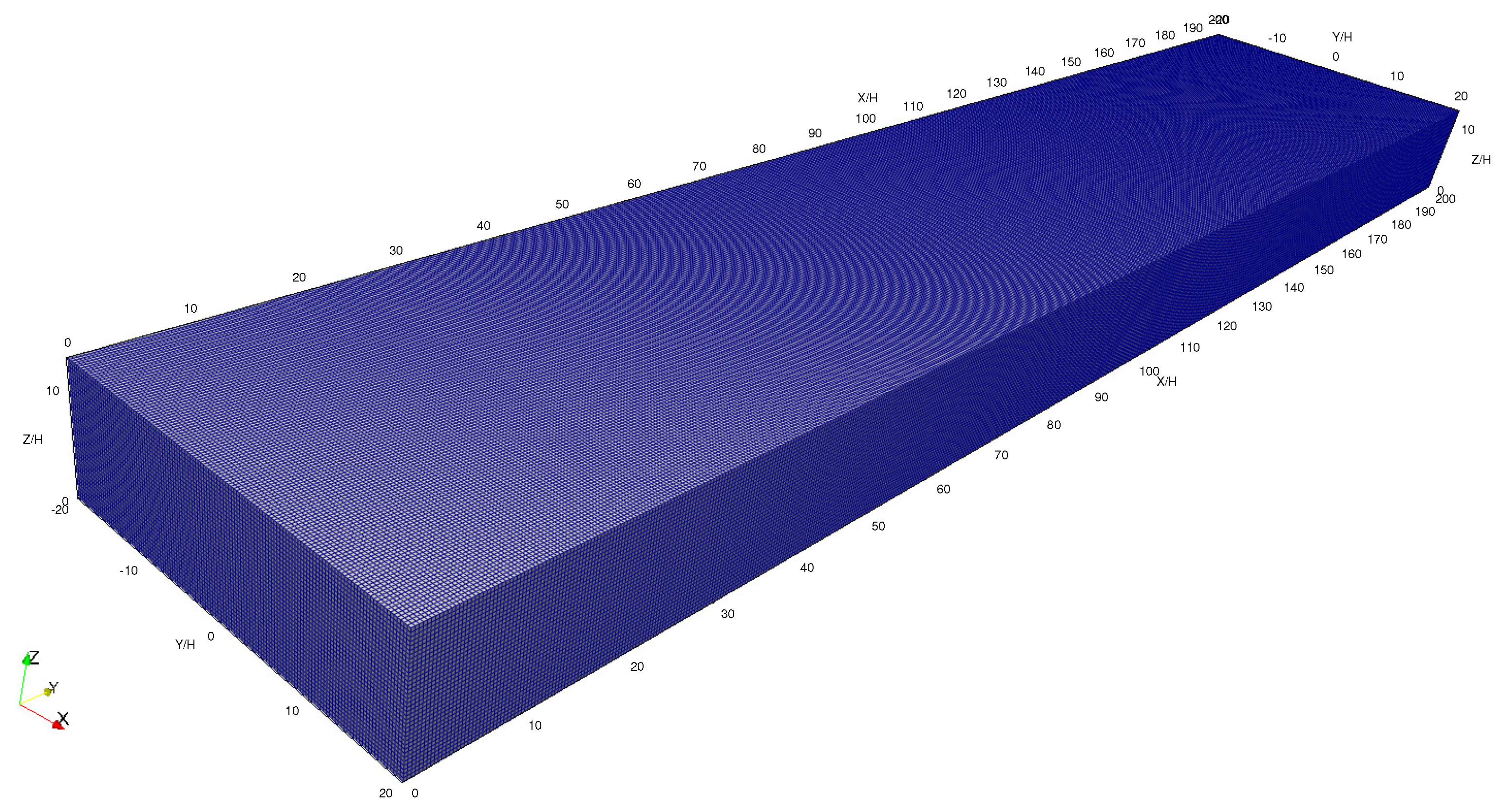
The computational grid is shown in Figure 2. The grid is uniform, made up of $\mathrm{5,340,168}$ hexahedra. The landfill is modeled as a square patch of size $\mathrm{H}$. The domain dimensions are $25\mathrm{H}$ in the vertical direction $\left(z\right)$, $200\mathrm{H}$ in the axial direction $\left(x\right)$, and $40\mathrm{H}$ in the spanwise direction $\left(y\right)$ directions. The grid is uniform with stencils, respectively, $\delta x=0.33167H$, $\delta y=0.3252H$, and $\delta z=0.3472H$.

In this work, the geometry of the topography has been neglected. This is due to the fact that the domain studied is very large. The approximation made here is that the characteristic landfill dimension $\mathrm{H}$ is much larger than the characteristic difference in altitude of the topography, namely $ϵ$, so that $ϵ/H<<1$. This implies that the topography behaves as a rugosity on the ground that has the effect of increasing vortex shedding from the wall and can be taken into account by increasing the turbulent Schmidt numbers in the LES model. However, this hypothesis is not always verified. The presence of a mountain or a gorge nearby can make this hypothesis not realistic.

2.3. Boundary Conditions

At the inlet $(x=0)$, a uniform axial velocity has been set. The mass flux of methane is defined as

$$\overline{J}=-{\left.D{\displaystyle \frac{\partial \overline{c}}{\partial z}}\right|}_{z=0}$$

(11)

The methane flux $\overline{J}$ is set to be zero everywhere except at a small, square surface of the landfill. This condition could be problematic, as it is unable to limit the concentration to physical values. However, if the mass flux is small enough, this problem is experienced only after a long period of time, possibly smaller than the duration of the simulation. The wind velocity profile has also been imposed at the inlet with the logarithmic formula

$$U_{inlet}={\displaystyle \frac{u_{\tau }}{\kappa }}log\left(1+{\displaystyle \frac{z}{z_0}}\right)$$

(12)

where

$$u_{\tau }=\sqrt{{\displaystyle \frac{{\tau }_0}{{\rho }_{air}}}}$$

(13)

and, to be consistent with the shear stress on the ground,

$$z_0={\displaystyle \frac{\nu }{u_{\tau }\kappa }}$$

(14)

In conclusion, the basis for the roughness length $z_0$ value is the boundary layer theory: ${\tau }_0={\rho }_{air}{u}_{\tau }^2$.

3. Results

The results will be organized in the following subsections: Section 3.1 describes the instantaneous concentration field with the velocity vectors for illustrative purposes; Section 3.2 discusses the velocity ad concentration vertical profiles and their properties; in Section 3.3, the LES results are used to derive a Gaussian plume model. The simulations used an adaptaive timestep. At each timestep, the maximum Courant number is set to be $<0.5$ for time stability, while the typical value of the resdiuals at each iteration for the velocity and concentration was in the range $[1·{10}^{-7}-5·{10}^{-7}]$, and the value of the residuals for the pressure was in the range $[1.5·{10}^{-5}-2.5·{10}^{-5}]$.

3.1. Fields

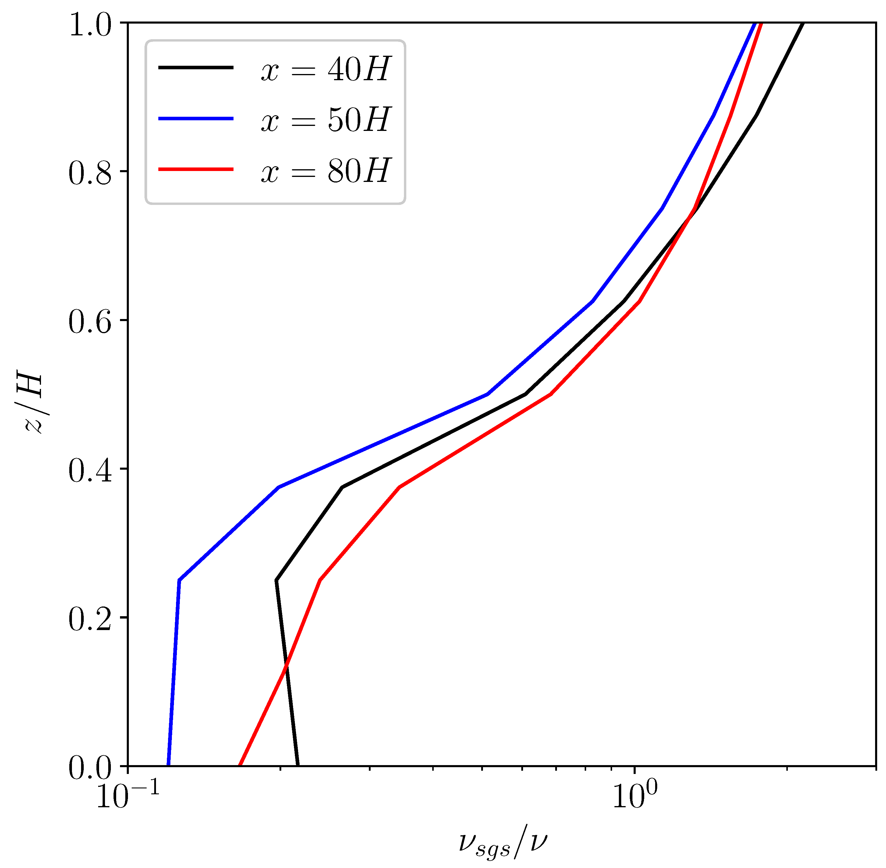
In order to demonstrate the accuracy of the near-wall grid, the scaled sub-grid viscosity is reported in Figure 3 in analogy with [44]. In an LES, the small scales are not resolved, like in the DNS, but are accounted for by the subgrid modeling. The sub-grid correction can be measured by the sub-grid viscosity: The bigger it is, the more the results are affected by the LES model. In Figure 3, it can be clearly seen that ${\nu }_{sgs}/\nu <1$ in the near-wall region. This means that the turbulent scales are well resolved in this region and that the grid stencil and shape are fit for purpose.

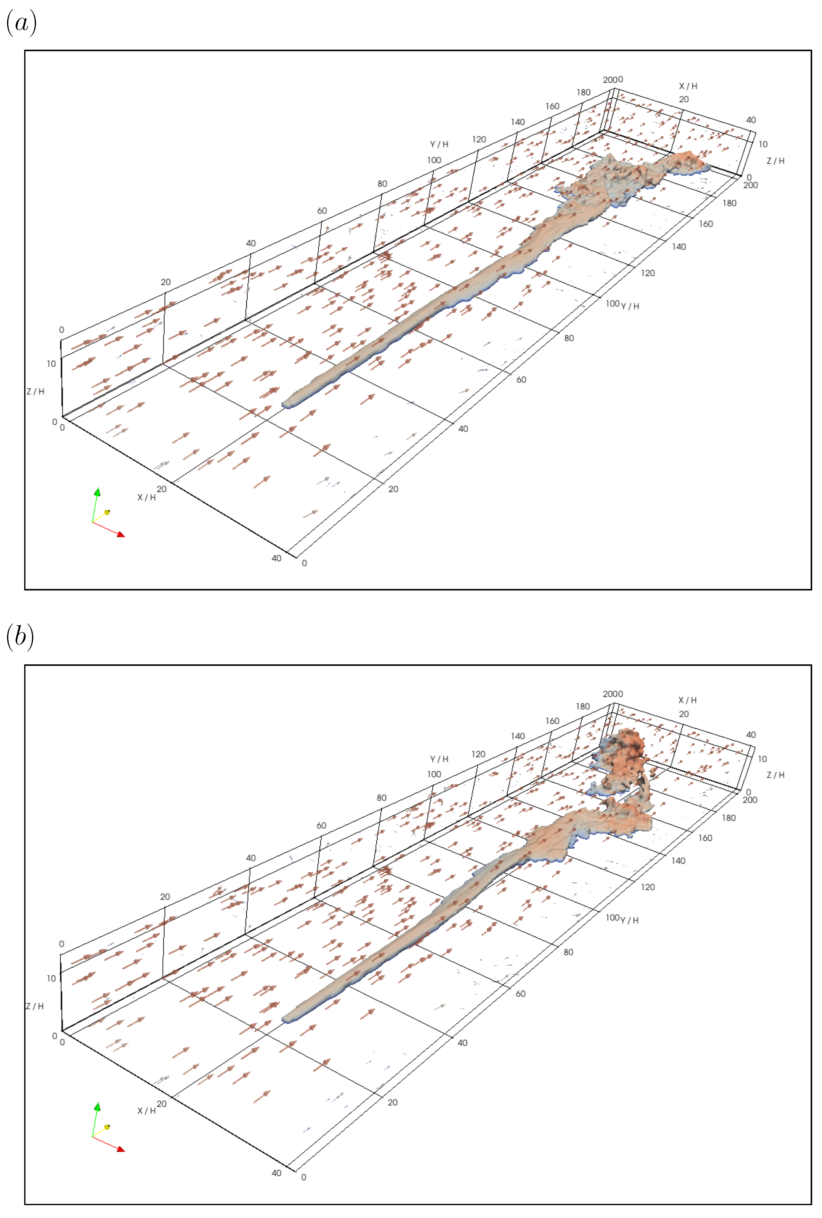
The iso-surfaces of the instantaneous concentration are shown in Figure 4. The results are reported at four dimensionless instants of time along with the instantaneous velocity vectors.

The instantaneous field is reported to show the transient nature of the emissions, due to turbulence instabilities in the boundary layer. The concentration field originates from the landfill and propagates along the wind direction. Because methane is emitted in the atmosphere through diffusion, most of it remains in the viscous sublayer for a long distance. Considering $U_{\infty }$ the unperturbed wind speed, methane starts diffusing in the atmosphere by convection at a distance equivalent to $Re\left(x\right)\simeq U_{\infty }x/\nu =\mathrm{1,734,650}$.

3.2. Profiles

The mean velocity profile can be expressed in terms of the self-similar variable ${\eta }_g$, defined as

$${\eta }_g=\left({\displaystyle \frac{u_{\tau }}{U_{\infty }}}\right){\displaystyle \frac{z}{\delta \left(x\right)}}$$

(15)

where $\delta \left(x\right)$ is the displacement thickness, defined as

$$\delta \left(x\right)={\int }_0^{\infty }\left(1-{\displaystyle \frac{U}{U_{\infty }}}\right)dz$$

(16)

while the self-similar velocity is defined as

$$f^{\prime }\left({\eta }_g\right)={\displaystyle \frac{U_{\infty }-U}{u_{\tau }}}$$

(17)

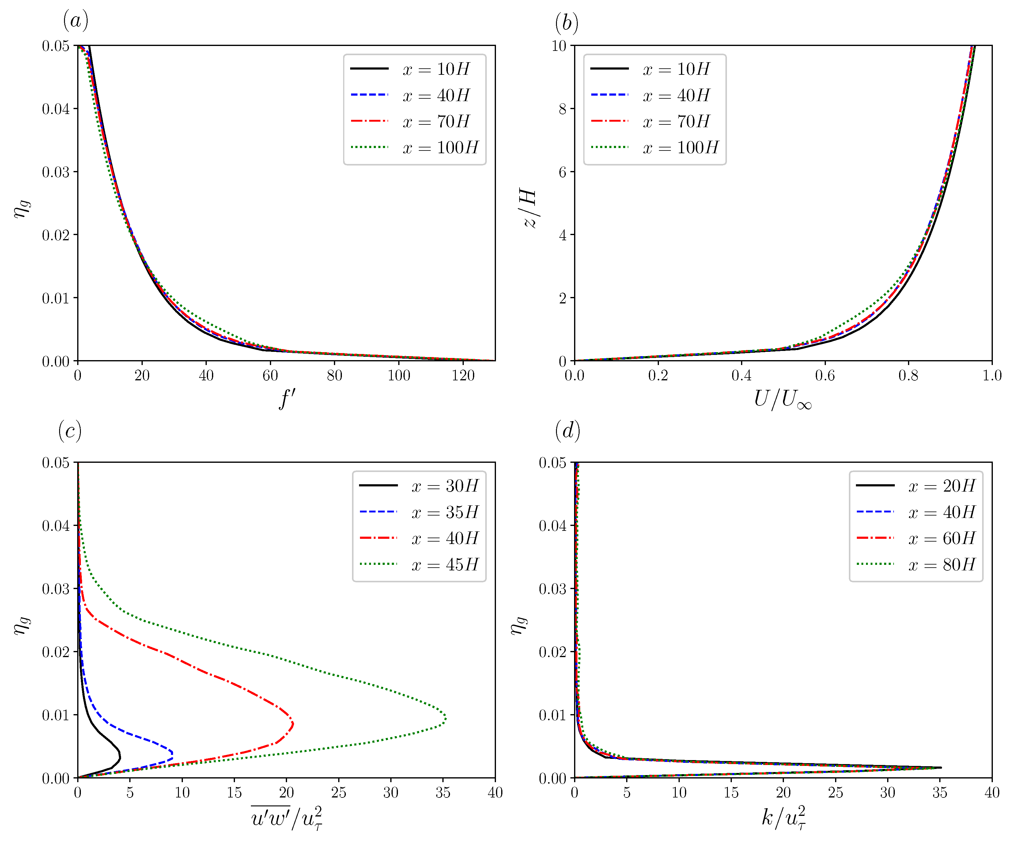
The mean velocity profile is logarithmic in first approximation. However, as shown in Figure 5b, there is a very slow axial evolution. The self-similar velocity $f^{\prime }$, defined in Equation (17), is shown to be independent from the axial position. This definition has the advantage of representing an infinite profile of a finite domain.

As far as turbulence is concerned, in Figure 5, two profiles are shown: the Reynolds shear stress $\overline{u^{\prime }{w}^{\prime }}$ in Figure 5c, and the turbulent kinetic energy k in Figure 5d. In Figure 5c, the Reynolds shear-stress profile shows a growth with the distance from the landfill. The Reynolds shear stress is null on the ground, because of the no-slip boundary condition, and it is null in the free stream, since it is outside the boundary layer. The Reynolds shear stress has its maximum close to the ground, moving outwards as the distance from the landfill grows.

On the other hand, the turbulent kinetic energy profile is essentially constant, as is the mean velocity. This is due to the fact that the turbulent kinetic energy acts hydrostatically on the flow and is balanced by the static pressure. The turbulent kinetic energy is positive by definition, null on the ground, because of the no-slip boundary condition, and null in the free stream, outside the boundary layer. Another interesting fact is that the turbulent kinetic energy is concentrated in a thin sub-layer, near the ground.

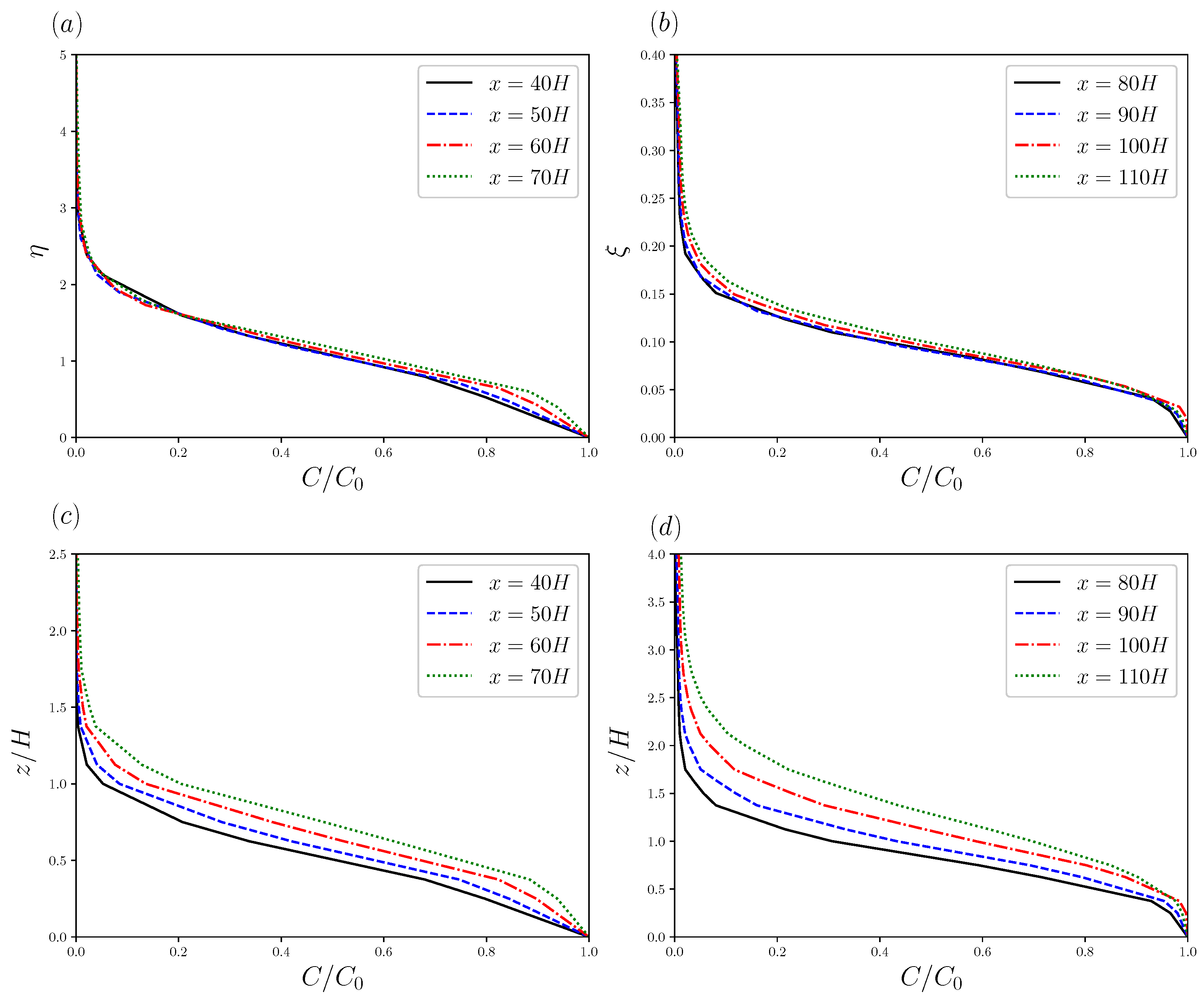
The mean concentration profile, scaled by the concentration on the ground, which can be referred to as the scaled concentration profile, is shown in Figure 6. The results show that the scaled concentration profile is self-similar. However, between $x=70H$ and $x=80H$, the self-similarity law changes. This behavior is similar to what is observed in the literature [42,43,44,45]. Closer to the landfill, the scaled-concentration profile is a function of the coordinate $\eta$, defined as

$$\eta =z\sqrt{{\displaystyle \frac{U_{\infty }}{\nu x}}}$$

(18)

while further down, the scaled-concentration profile is a function of the variable $\xi$, defined as

$$\xi ={\displaystyle \frac{z}{ax}}$$

(19)

where $a=0.13$. The dependency on the variable $\eta$ indicates the region in which the methane spreading is dominated by molecular diffusion, whereas the dependency on the variable $\xi$ indicates the region in which turbulent diffusion is dominant. The self-similar profiles are compared with the profile along the vertical axis.

In particular, Figure 5a should be compared with Figure 5c, while Figure 5b should be compared with Figure 5d. In both cases, the scaled concentration profile is shown to spread more along the vertical axis at increasing distances from the landfill. Figure 5a,b show that it is possible to bring the profiles into congruence by transforming the coordinates, although different transformations have to be used in different regions, in analogy with [42,43,44,45]. This simplifies the modeling since the scaled concentration profile depends only on the self-similar coordinate.

In Figure 7, the profiles of the concentration root mean square, $c_{rms}$, defined as:

$$c_{rms}=\sqrt{\overline{c^{\prime }{c}^{\prime }}}$$

(20)

scaled by the mean concentration on the ground, $C_0$, and the friction concentration $c_{\tau }$, defined as

$$c_{\tau }={\displaystyle \frac{\nu }{u_{\tau }}}{\left|{\displaystyle \frac{\partial C}{\partial z}}\right|}_0,$$

(21)

are shown. In Figure 7a,b, the concentration root mean square, scaled by the concentration on the ground, is shown.

This variable does not show self-similarity with respect to the coordinate $\eta$. In Figure 7a, the scaled concentration increases with the distance from the landfill, but this is a scale effect, since the ground concentration diminishes with the distance as well. In Figure 7b, the scaled profile is independent from the axial coordinate, showing a self-similarity to the coordinate $\xi$. In both figures, the profile shows a maximum on the ground and decays monotonically in the free stream.

In Figure 7c,d, the concentration root mean square, scaled by the friction concentration, is shown. In this case, the scaled concentration is not self-similar, neither with respect to the coordinate $\eta$ nor with respect to the coordinate $\xi$. This is due to the fact that the friction concentration decays more rapidly than the concentration on the ground, whereas the root mean square of the concentration and the mean concentration at the ground decay at the same rate, at least for $x>70H$. The lack of self-similarity with respect to the variable $\eta$ is not unexpected since the concentration root mean square is a turbulent field and it should not be dominated by the diffusive effect, whereas the self-similarity with respect to the coordinate $\xi$ is reasonable since this coordinate takes into account turbulent diffusion.

3.3. Gaussian Model

The concentration field is widely modeled as a Gaussian curve [28,38,46,47,48,49,50,51]. In this work, we adopt the definition in Equation (22):

$$C(x,y,z)=A\left(x\right)exp\left(-{\displaystyle \frac{{\left(z-\mu \left(x\right)\right)}^2}{2{\sigma }_z^2\left(x\right)}}-{\displaystyle \frac{y^2}{2{\sigma }_y^2\left(x\right)}}\right)$$

(22)

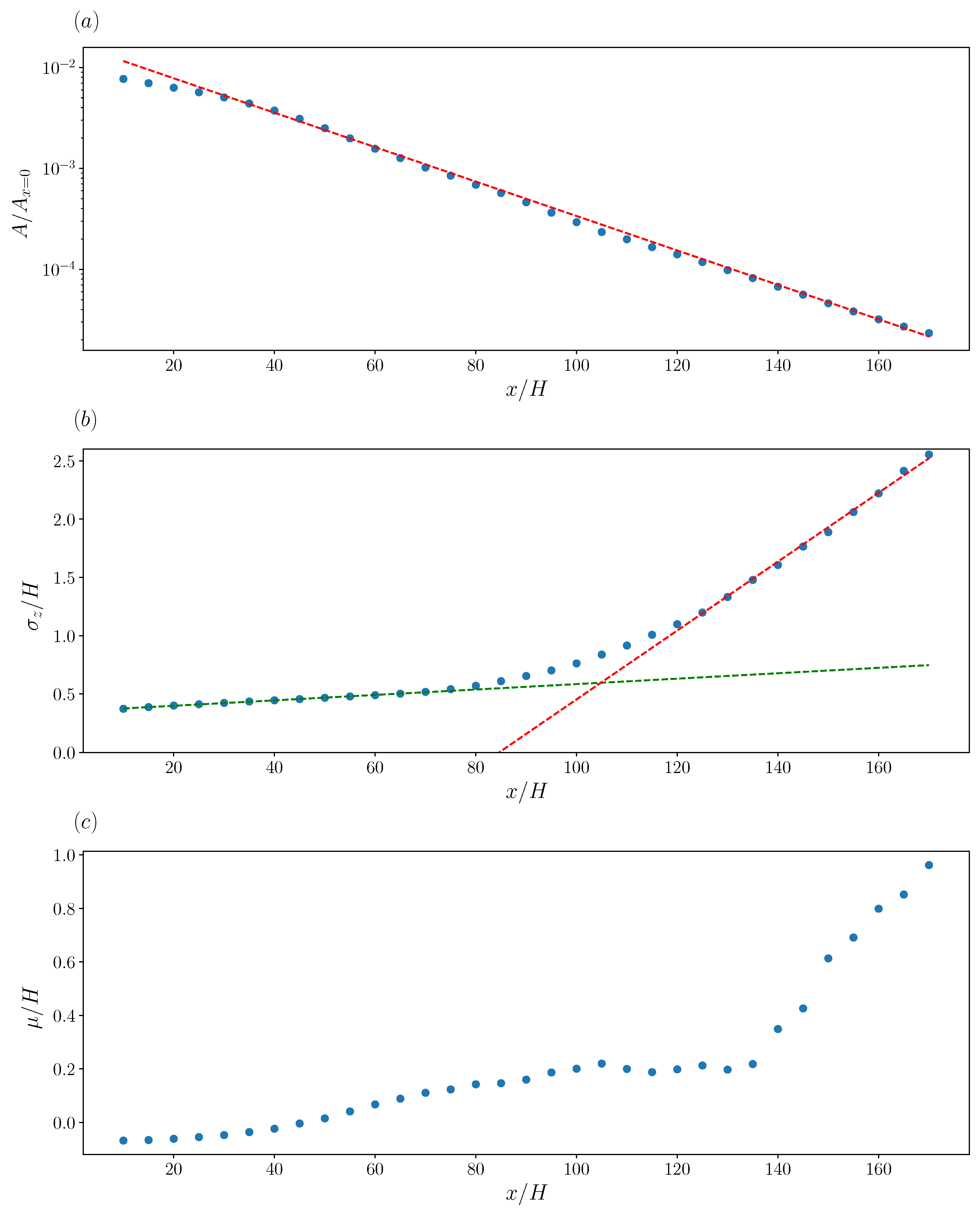
where $A\left(x\right)$ is the highest concentration, $\mu \left(x\right)$ is the coordinate at which the maximum concentration is found, and ${\sigma }_z\left(x\right)$ is the vertical standard deviation of the concentration profile. These parameters have been extrapolated from the data through regression analysis of the profiles, using the curve_fit of the scipy package of the Python language. In Figure 8, these three parameters are reported at different distances from the landfill.

In Figure 8a, the concentration amplitude, scaled by the concentration at the landfill, i.e., $A\left(0\right)$, is reported. This parameter is scaled since the actual value depends on the methane concentration in the landfill. The parameter $A\left(x\right)$ decays exponentially with the distance and the decay is not affected by the distance from the landfill.

The vertical standard deviation ${\sigma }_z\left(x\right)$ in Figure 8b shows an interesting behavior. It increases at the increasing distance, but between $x/H>80$ and $x/H<120$, the rate of growth increases 10 fold. This indicates the transition from a molecular diffusion dominant region to a turbulence-dominated region. In both regions, the vertical standard deviation can be approximated by a linear function of the coordinates, i.e., ${\sigma }_z\left(x\right)=A·H+B·x$, where A and B are dimensionless coefficients. The results indicate that the slop grows about 12.7 times between the diffusive region and the turbulent region.

The last parameter to consider is the mean, $\mu \left(x\right)$, corresponding to the vertical coordinate at which the mean concentration is the highest. Usually, this parameter is set equal to 0, since it is reasonable to assume that the greatest concentration is found on the ground. Nevertheless, the present results show that this parameter increases with the increasing distance from the landfill. This is probably due to the buoyancy that mixes methane and air. In analogy with the vertical standard deviation, the slope increases rapidly. However, this occurs for $x>140H$. Since methane is well within the turbulent region at this point, this sudden increase should be due to the buoyancy. Unfortunately, the pattern is difficult to model, since it is neither linear nor exponential. There is a need for further modeling of the $\mu \left(x\right)$ parameter, since at $x=180H$, the mean is approximately equal to the landfill size; this is significant given the interest in ground level concentrations at which humans could be exposed. However, at this distance, the concentration on the ground is about ${10}^{-5}$ smaller than the concentration in the landfill, and the concentration levels are not considered harmful.

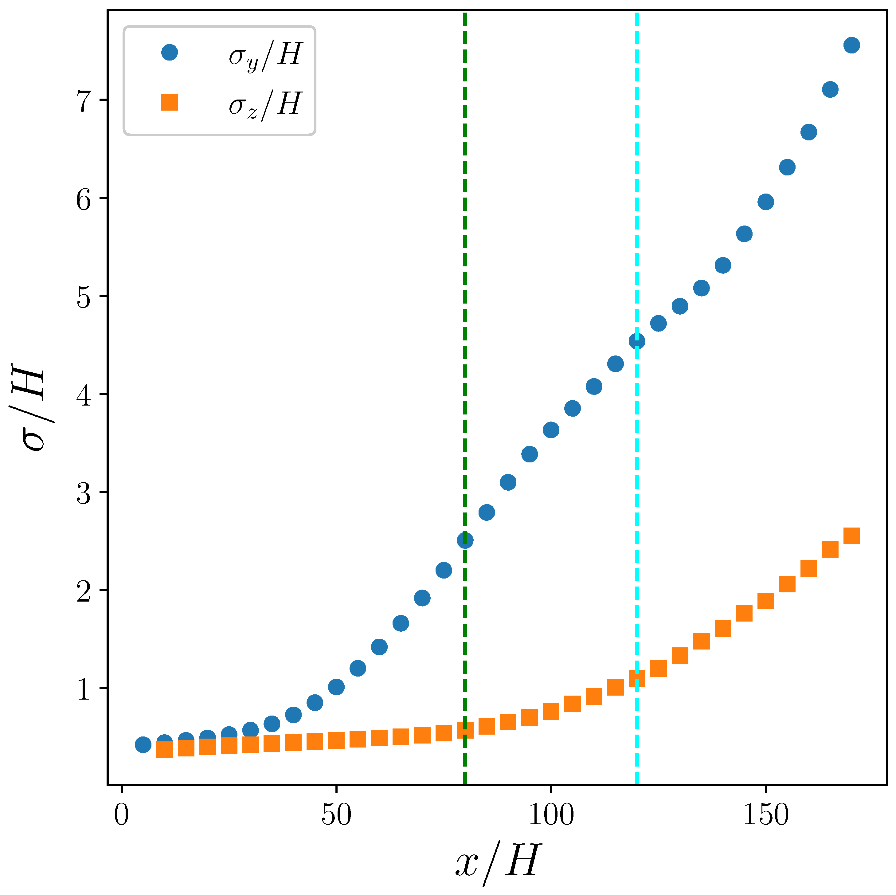
In Figure 9, both the vertical and the spanwise standard deviation are reported. The LES results indicate that, despite being in the neighborhood of the landfill, i.e., $x<25H$, the two standard deviations are comparable; the spanwise standard deviation grows faster compared to the vertical one. In fact, at $x=100H$, the spanwise standard deviation is about five times bigger than the vertical standard deviation. This is due to the fact that on the ground, diffusion in the spanwise direction is allowed, while both convection and diffusion are not allowed. Nevertheless, it is expected that with the increasing wind speed, the vertical standard deviation will increase as well.

4. Discussion and Conclusions

The present study reveals a few details of methane emissions from landfills that can be used in determining the optimal position of atmospheric receptors. In this work, the domain considered is very large, about 180 times the size of the landfill. However, the results show that the concentration drops sharply with the distance. In the first 10 landfill diameters, the concentration of ${\mathrm{CH}}_4$ on the ground is reduced by more than 100 fold.

In this study, the focus is on the buoyancy and the far-field effects of methane emissions. In particular, the mean axial velocity of the wind is found to be self-similar with respect to the coordinate ${\eta }_g$, defined in Equation (15). The velocity profile is approximated by a logarithmic function but this does not correspond to the far-field solution. As far as the mean concentration is concerned, this field is found to be self-similar if scaled with its value on the ground.

The concentration on the ground is found to decay exponentially with the distance in Figure 8a. This fact is important in modeling, and it will make it easy to derive a self-similar model for the scaled concentration, since the ratio between the wall concentration and its axial derivative is constant. The scaled concentration profile is, indeed, found to be self-similar with respect to two self-similar coordinates: $\eta$, defined in Equation (18), and $\xi$, defined in Equation (19). The dependency from the coordinate $\eta$ is shown for $x<70H$, while the dependency from the coordinate $\xi$ is shown for $x>80H$. This is consistent with the self-similar behavior in the jet flow [42,43,44,45]. However, it is surprising that the velocity field is self-similar to a different coordinate, i.e., ${\eta }_g$, with respect to the scaled concentration profile, respectively, $\eta$ and $\xi$. This might indicate that the displacement thickness might be proportional to $\sqrt{x}$ for $x<70H$, and proportional to x for $x>80H$. The results of the concentration root mean square profile are also shown. This variable is scaled by the mean concentration on the ground (Figure 7a,b) and the friction concentration (Figure 7c,d). Interestingly, only the concentration rms, scaled by the mean concentration on the ground, is shown to be self-similar with respect to the coordinate $\xi$.

The LES results have been used to fit a Gauss dispersion model, defined in Equation (22). The amplitude $A\left(x\right)$ and the vertical standard deviation ${\sigma }_z\left(x\right)$ fit well, respectively, with an exponential and a linear function of the distance from the coordinates. The mean vertical coordinate $\mu \left(x\right)$, on the other hand, grows slowly with the distance from the landfill but does not seem to fit a simple model. The evolution of this variable is probably due to buoyancy, although further simulations will need to confirm this. Nevertheless, this parameter seems negligible.

The main result of this work consists in having found a self-similar behavior for methane diffusion from landfills in the far field. Self-similarity (or self-preservation) occurs when the profiles of a given field can be brought into congruence by simple scale factors that depend on the coordinates. A consequence of self-similarity is that the evolution of a field can be described by a reduced number of coordinates, or, in some cases, by only one. This reduces the field transport equation to an ordinary differential equation, whose solution can be obtained at a reduced computational cost. Applied to the landfill, this means that, potentially, only two arrays of sensors will have to be used to accurately estimate the emission rates: one between $x=10H$ and $x=70H$, and the other for $x>80H$. Furthermore, the results in Figure 6 show that to capture $80\%$ of the concentration field, the highest atmospheric receptor should be located at a distance from the ground equivalent to the landfill size.

Our finding of an increase in the height of a plume with buoyancy is consistent with the methane measurements taken at a landfill site using a drone [23]. The results reported there show much greater variability than we find, indicating that other small-scale factors such as turbulence or changes in wind speeds are also playing an important role. A reduced signal-to-noise ratio would, thus, be expected in studies of similar plumes using surface-based measurements. An implication of this is that any gain in the sample height (e.g., using towers or poles) would increase the quality of the emission estimates. A second implication is that the existing surface-based estimates, e.g., [50], may be underestimating the actual emission because the lower edge of the plume is being sampled, not the core. Finally, improved emission estimates might be generated if Gaussian plume models could be modified to allow for buoyancy.

Nevertheless, the present results suffer from a few limitations, due to the topography, the wind speed, and the methane flux boundary condition from the landfill.

This work can be summarized as follows:

• In this work, an ideal topography has been used. The ground is modeled as a flat surface. In reality, the area around the landfill is not flat since it is made of hills, valleys, roads, and buildings. Nevertheless, considering the characteristic size of the canopy $ϵ$, the ratio $ϵ/H$ can be much smaller than 1. In that case, the site topography can be modeled as a roughness and be taken into account in a single parameter, namely, the turbulent Schmidt number ${\sigma }_C$ for the mean concentration. The foreseen effect is that this will change the boundaries of the turbulent region so that the mean concentration will be self-similar for some x smaller than $80H$, but it is unlikely that this will affect methane dispersion in the far field. Of course, this will not be true if the size of the landfill is comparable with the characteristic size of the topography.
• The second limitation consists in the wind speed. Knowing the fluid dynamic conditions is fundamental in order to interpret the sampling results and estimate emission rates. However, the wind speed can vary significantly and because of buoyancy, the velocity profile is influenced by the methane concentration itself. Nevertheless, it is reasonable to assume that, regardless of the speed, the mean velocity profile remains approximately logarithmic. The difference could be that at higher speeds, the region in which the mean concentration is self-similar to the coordinate $\xi$ would be shorter and the dependency from the coordinate $\xi$ would occur earlier. Overall, a different wind speed should not change the results obtained in this work. It is worth mentioning that there is one factor of uncertainty that concerns buoyancy. Buoyancy makes ${\mathrm{CH}}_4$ concentration an active scalar. This means that methane concentration influences the flow field. Nevertheless, as the ${\mathrm{CH}}_4$ mass fraction is small relative to air, this effect should be negligible.
• The third limitation consists in the modeling of the methane influx. Methane is emitted in the landfill by a diffusive flux, since there is no air flux from the ground to the atmosphere. In this work, a Neumann boundary condition, i.e., constant flux of ${\mathrm{CH}}_4$, has been imposed on the landfill. However, this condition represents a simplification. In reality, the flux of methane would depend on the concentration of ${\mathrm{CH}}_4$ on the landfill. However, determining experimentally the relationship between methane flux and methane concentration can be a difficult process. Computational fluid dynamics could help this process by a trial and error process, but this was outside the scope of this work.

This work has determined a self-similar dependency between the mean methane concentration and specific combination of the axial and vertical coordinates. This information is powerful because, if confirmed, it would reduce the number of measurement sites needed. Further simulations are required to confirm this behavior at different wind speeds and with a better modeling of methane emission from the landfill into the atmosphere. This methodology could be extended to other problems, such as methane emissions from pipelines [52,53,54,55,56]. The scaled mean concentration exhibits two self-similar behaviors consistent with what is found in case of a round and rectangular jet with low inlet velocity. The present results can be used to improve Gaussian dispersion modeling. For example, further studies could assess the influence of the wind speed and improve the modeling of the methane emission boundary condition.

References

1. Peng, M.Q.; Chen, T.H.; Jin, T.; Su, Y.C.; Luo, S.T.; Xu, H. A Novel First-Order Kinetic Model for Simultaneous Anaerobic–Aerobic Degradation of Municipal Solid Waste in Landfills. Processes 2024, 12, 2225. [Google Scholar] [CrossRef]
2. Huang, D.; Du, Y.; Xu, Q.; Ko, J.H. Quantification and control of gaseous emissions from solid waste landfill surfaces. J. Environ. Manag. 2022, 302, 114001. [Google Scholar] [CrossRef] [PubMed]
3. Weng, B. The road to climate change mitigation via methane emissions monitoring. Nat. Rev. Electr. Eng. 2024, 1, 69–70. [Google Scholar] [CrossRef]
4. Li, K.; Xu, W.; Chen, Y.; Zhan, L.; Ke, H.; Xu, H.; Xiao, D. Biochemical, hydrological and mechanical behaviors of high food waste content MSW landfill: Numerical simulation analysis of a large-scale experiment. Waste Manag. 2023, 171, 557–567. [Google Scholar] [CrossRef]
5. Pan, Q.; Liu, Q.Y.; Zheng, J.; Li, Y.H.; Xiang, S.; Sun, X.J.; He, X.S. Volatile and semi-volatile organic compounds in landfill gas: Composition characteristics and health risks. Environ. Int. 2023, 174, 107886. [Google Scholar] [CrossRef]
6. Wu, T.; Cheng, J.; Wang, S.; He, H.; Chen, G.; Xu, H.; Wu, S. Hotspot Detection and Estimation of Methane Emissions from Landfill Final Cover. Atmosphere 2023, 14, 1598. [Google Scholar] [CrossRef]
7. Stadler, C.; Fusé, V.S.; Linares, S.; Guzmán, S.A.; Juliarena, M.P. Accessible sampling methodologies to quantify the net methane emission from landfill cells. Atmos. Pollut. Res. 2024, 15, 102011. [Google Scholar] [CrossRef]
8. Gallego, E.; Perales, J.; Aguasca, N.; Domínguez, R. Determination of emission factors from a landfill through an inverse methodology: Experimental determination of ambient air concentrations and use of numerical modelling. Environ. Pollut. 2024, 351, 124047. [Google Scholar] [CrossRef]
9. Li, R.; Yuan, J.; Li, X.; Zhao, S.; Lu, W.; Wang, H.; Zhao, Y. Health risk assessment of volatile organic compounds (VOCs) emitted from landfill working surface via dispersion simulation enhanced by probability analysis. Environ. Pollut. 2023, 316, 120535. [Google Scholar] [CrossRef]
10. Gunarathne, V.; Phillips, A.J.; Zanoletti, A.; Rajapaksha, A.U.; Vithanage, M.; Di Maria, F.; Pivato, A.; Korzeniewska, E.; Bontempi, E. Environmental pitfalls and associated human health risks and ecological impacts from landfill leachate contaminants: Current evidence, recommended interventions and future directions. Sci. Total Environ. 2024, 912, 169026. [Google Scholar] [CrossRef]
11. Fosco, D.; De Molfetta, M.; Renzulli, P.; Notarnicola, B. Progress in monitoring methane emissions from landfills using drones: An overview of the last ten years. Sci. Total Environ. 2024, 945, 173981. [Google Scholar] [CrossRef] [PubMed]
12. Wu, T.; Yang, H.; Cheng, J.; Chen, G.; Xu, H.; Zhang, L. Theoretical Analysis of Landfill Gas Migration in Capillary Barrier Covers Considering Effects of Waste Temperature. Appl. Sci. 2024, 14, 9473. [Google Scholar] [CrossRef]
13. Wang, Q.; Gu, X.; Tang, S.; Mohammad, A.; Singh, D.N.; Xie, H.; Chen, Y.; Zuo, X.; Sun, Z. Gas transport in landfill cover system: A critical appraisal. J. Environ. Manag. 2022, 321, 116020. [Google Scholar] [CrossRef] [PubMed]
14. Wójtowicz-Wróbel, A.; Kania, O.; Kocewiak, K.; Wójtowicz, R.; Dzierwa, P.; Trojan, M. Thermal-flow calculations for a thermal waste treatment plant and CFD modelling of the spread of gases in the context of urban structures. Energy 2023, 263, 125952. [Google Scholar] [CrossRef]
15. Olaguer, E.P.; Jeltema, S.; Gauthier, T.; Jermalowicz, D.; Ostaszewski, A.; Batterman, S.; Xia, T.; Raneses, J.; Kovalchick, M.; Miller, S.; et al. Landfill emissions of methane inferred from unmanned aerial vehicle and mobile ground measurements. Atmosphere 2022, 13, 983. [Google Scholar] [CrossRef]
16. Global Assessment: Urgent Steps Must Be Taken to Reduce Methane Emissions This Decade. Available online: https://unfccc.int/news (accessed on 21 January 2024).
17. Wang, Y.; Song, W.; Wang, Q.; Yang, F.; Yan, Z. Predicting Enteric Methane Emissions from Dairy and Beef Cattle Using Nutrient Composition and Intake Variables. Animals 2024, 14, 3452. [Google Scholar] [CrossRef]
18. Mønster, J.; Kjeldsen, P.; Scheutz, C. Methodologies for measuring fugitive methane emissions from landfills—A review. Waste Manag. 2019, 87, 835–859. [Google Scholar] [CrossRef]
19. Xia, T.; Borjigin, S.G.; Raneses, J.; Stroud, C.A.; Batterman, S.A. Mobile measurements of atmospheric methane at eight large landfills: An assessment of temporal and spatial variability. Atmosphere 2023, 14, 906. [Google Scholar] [CrossRef]
20. Connor, A.; Shaw, J.T.; Yarrow, N.; Howes, N.; Helmore, J.; Finlayson, A.; Barker, P.; Robinson, R. A framework for describing and classifying methane reporting requirements, emission sources, and monitoring methods. Environ. Sci. Atmos. 2024, 4, 1203–1217. [Google Scholar] [CrossRef]
21. Bell, C.; Rutherford, J.; Brandt, A.; Sherwin, E.; Vaughn, T.; Zimmerle, D. Single-blind determination of methane detection limits and quantification accuracy using aircraft-based LiDAR. Elem. Sci. Anthr. 2022, 10, 00080. [Google Scholar] [CrossRef]
22. Esparza, Á.E.; Rowan, G.; Newhook, A.; Deglint, H.J.; Garrison, B.; Orth-Lashley, B.; Girard, M.; Shaw, W. Analysis of a tiered top-down approach using satellite and aircraft platforms to monitor oil and gas facilities in the Permian basin. Renew. Sustain. Energy Rev. 2023, 178, 113265. [Google Scholar] [CrossRef]
23. Yong, H.; Allen, G.; Mcquilkin, J.; Ricketts, H.; Shaw, J.T. Lessons learned from a UAV survey and methane emissions calculation at a UK landfill. Waste Manag. 2024, 180, 47–54. [Google Scholar] [CrossRef] [PubMed]
24. Wigle, A.; Béliveau, A.; Blackmore, D.; Lapeyre, P.; Osadetz, K.; Lemieux, C.; Daun, K.J. Estimation and Applications of Uncertainty in Methane Emissions Quantification Technologies: A Bayesian Approach. ACS Es&t Air 2024, 1, 1000–1014. [Google Scholar]
25. Lucernoni, F.; Rizzotto, M.; Tapparo, F.; Capelli, L.; Sironi, S.; Busini, V. Use of CFD for static sampling hood design: An example for methane flux assessment on landfill surfaces. Chemosphere 2016, 163, 259–269. [Google Scholar] [CrossRef] [PubMed]
26. Kia, S.; Flesch, T.K.; Freeman, B.S.; Aliabadi, A.A. Calculating gas emissions from open-pit mines using inverse dispersion modelling: A numerical evaluation using CALPUFF and CFD-LS. J. Wind. Eng. Ind. Aerodyn. 2022, 226, 105046. [Google Scholar] [CrossRef]
27. Christo, F.; Fletcher, D.; Joseph, S. Computational fluid dynamics modelling of a landfill gas flare. J. Inst. Energy 1998, 71, 145–151. [Google Scholar]
28. Samec, N.; Hriberšek, M.; Ravnik, J. Numerical simulation of particle air dispersion around the landfill. Air Pollut. XVII 2009, 123, 27. [Google Scholar]
29. Alizadehdakhel, A.; Zoqi, M. A CFD investigation on the effect of CO2 injection into a landfill. In Proceedings of the 2010 International Conference on Chemical Engineering and Applications, Singapore, 26–28 February 2010; pp. 176–180. [Google Scholar]
30. Hriberšek, M.; Samec, N.; Ravnik, J.; Zadravec, M. Numerical Simulations of Wind Induced Particle Contamination in Gypsum Landfill Surroundings. Environ. Model. Assess. 2011, 16, 479–489. [Google Scholar] [CrossRef]
31. Sanchez, R.; Tsotsis, T.T.; Sahimi, M. Computer simulation of gas generation and transport in landfills. IV: Modeling of liquid–gas flow. Chem. Eng. Sci. 2010, 65, 1212–1226. [Google Scholar] [CrossRef]
32. White, J.; Nayagum, D.; Beaven, R. A multi-component two-phase flow algorithm for use in landfill processes modelling. Waste Manag. 2014, 34, 1644–1656. [Google Scholar] [CrossRef]
33. Halvorsen, D.; Nec, Y.; Huculak, G. Horizontal landfill gas wells: Geometry, physics of flow and connection with the atmosphere. Phys. Chem. Earth Parts A/B/C 2019, 113, 50–62. [Google Scholar] [CrossRef]
34. Zheng, Q.T.; Feng, S.J.; Wu, S.J.; Zhang, X.L.; Chen, H.X. Modeling of multifield coupling interactions in an aerobic landfill based on the finite volume method. Comput. Geotech. 2022, 146, 104704. [Google Scholar] [CrossRef]
35. Guo, S.; Yu, W.; Zhao, H.; Lai, C.; Bian, S.; Jin, P.; Liang, S.; Yuan, S.; Huang, L.; Wang, S.; et al. Numerical simulation to optimize passive aeration strategy for semi-aerobic landfill. Waste Manag. 2023, 171, 676–685. [Google Scholar] [CrossRef] [PubMed]
36. Torno, S.; Toraño, J.; Menendez, M.; Gent, M.; Allende, C.; Popov, V.; Itoh, H.; Mander, U.; Brebbia, C. LIDAR technique application to the analysis of environmental pollution. Waste Manag. Environ. V 2010, 140, 301. [Google Scholar]
37. Torno, S.; Toraño, J.; Menendez, M.; Gent, M.; Allende, C. Prediction of particulate air pollution from a landfill site using CFD and LIDAR techniques. Environ. Fluid Mech. 2011, 11, 99–112. [Google Scholar] [CrossRef]
38. Riddick, S.N.; Connors, S.; Robinson, A.D.; Manning, A.J.; Jones, P.S.; Lowry, D.; Nisbet, E.; Skelton, R.L.; Allen, G.; Pitt, J.; et al. Estimating the size of a methane emission point source at different scales: From local to landscape. Atmos. Chem. Phys. 2017, 17, 7839–7851. [Google Scholar] [CrossRef]
39. Leifer, I.; Melton, C.; Tratt, D.M.; Buckland, K.N.; Clarisse, L.; Coheur, P.; Frash, J.; Gupta, M.; Johnson, P.D.; Leen, J.B.; et al. Remote sensing and in situ measurements of methane and ammonia emissions from a megacity dairy complex: Chino, CA. Environ. Pollut. 2017, 221, 37–51. [Google Scholar] [CrossRef]
40. Kormi, T.; Mhadhebi, S.; Ali, N.B.H.; Abichou, T.; Green, R. Estimation of fugitive landfill methane emissions using surface emission monitoring and Genetic Algorithms optimization. Waste Manag. 2018, 72, 313–328. [Google Scholar]
41. Kumar, P.; Caldow, C.; Broquet, G.; Shah, A.; Laurent, O.; Yver-Kwok, C.; Ars, S.; Defratyka, S.; Gichuki, S.W.; Lienhardt, L.; et al. Detection and long-term quantification of methane emissions from an active landfill. Atmos. Meas. Tech. 2024, 17, 1229–1250. [Google Scholar] [CrossRef]
42. Petracci, I.; Angelino, M.; Di Venuta, I.; Boghi, A.; Gori, F. Experiments and numerical simulations of mass transfer and flow evolution in transient rectangular free jet of air. Int. Commun. Heat Mass Transf. 2019, 108, 104290. [Google Scholar] [CrossRef]
43. Di Venuta, I.; Boghi, A.; Petracci, I.; Bartoli, C.; Gori, F. Flow evolution and mass transfer in a turbulent rectangular free jet of air with small laminar Schmidt number. Int. Commun. Heat Mass Transf. 2019, 107, 44–54. [Google Scholar] [CrossRef]
44. Boghi, A.; Di Venuta, I.; Angelino, M.; Gori, F. Large eddy simulation and self-similarity analysis of the momentum spreading in the near field region of turbulent submerged round jets. Int. J. Heat Fluid Flow 2019, 80, 108466. [Google Scholar] [CrossRef]
45. Angelino, M.; Di Venuta, I.; Boghi, A.; Petracci, I.; Gori, F. Further results on the mean mass transfer and fluid flow in a turbulent round jet. Int. Commun. Heat Mass Transf. 2023, 141, 106568. [Google Scholar] [CrossRef]
46. Holmes, N.; Morawska, L. A review of dispersion modelling and its application to the dispersion of particles: An overview of different dispersion models available. Atmos. Environ. 2006, 40, 5902–5928. [Google Scholar] [CrossRef]
47. Gasbarra, D.; Toscano, P.; Famulari, D.; Finardi, S.; Di Tommasi, P.; Zaldei, A.; Carlucci, P.; Magliulo, E.; Gioli, B. Locating and quantifying multiple landfills methane emissions using aircraft data. Environ. Pollut. 2019, 254, 112987. [Google Scholar] [CrossRef] [PubMed]
48. Foster-Wittig, T.A.; Thoma, E.D.; Albertson, J.D. Estimation of point source fugitive emission rates from a single sensor time series: A conditionally-sampled Gaussian plume reconstruction. Atmos. Environ. 2015, 115, 101–109. [Google Scholar] [CrossRef]
49. Matacchiera, F.; Manes, C.; Beaven, R.; Rees-White, T.; Boano, F.; Mønster, J.; Scheutz, C. AERMOD as a Gaussian dispersion model for planning tracer gas dispersion tests for landfill methane emission quantification. Waste Manag. 2019, 87, 924–936. [Google Scholar] [CrossRef]
50. Riddick, S.N.; Mauzerall, D.L.; Celia, M.; Harris, N.R.; Allen, G.; Pitt, J.; Staunton-Sykes, J.; Forster, G.L.; Kang, M.; Lowry, D.; et al. Methane emissions from oil and gas platforms in the North Sea. Atmos. Chem. Phys. 2019, 19, 9787–9796. [Google Scholar] [CrossRef]
51. Manheim, D.C.; Newman, S.; Yeşiller, N.; Hanson, J.L.; Guha, A. Application of cavity ring-down spectroscopy and a novel near surface Gaussian plume estimation approach to inverse model landfill methane emissions. MethodsX 2023, 10, 102048. [Google Scholar] [CrossRef]
52. Lelieveld, J.; Lechtenböhmer, S.; Assonov, S.S.; Brenninkmeijer, C.A.; Dienst, C.; Fischedick, M.; Hanke, T. Low methane leakage from gas pipelines. Nature 2005, 434, 841–842. [Google Scholar] [CrossRef]
53. Boghi, A.; Brown, L.; Sawko, R.; Thompson, C.P. An inertial two-phase model of wax transport in a pipeline during pigging operations. Int. J. Multiph. Flow 2017, 94, 17–30. [Google Scholar] [CrossRef]
54. Yu, J.; Hmiel, B.; Lyon, D.R.; Warren, J.; Cusworth, D.H.; Duren, R.M.; Chen, Y.; Murphy, E.C.; Brandt, A.R. Methane emissions from natural gas gathering pipelines in the permian basin. Environ. Sci. Technol. Lett. 2022, 9, 969–974. [Google Scholar] [CrossRef] [PubMed]
55. Boghi, A.; Brown, L.; Sawko, R.; Thompson, C.P. A non-inertial two-phase model of wax transport in a pipeline during pigging operations. J. Pet. Sci. Eng. 2018, 165, 664–672. [Google Scholar] [CrossRef]
56. Weller, Z.D.; Hamburg, S.P.; von Fischer, J.C. A national estimate of methane leakage from pipeline mains in natural gas local distribution systems. Environ. Sci. Technol. 2020, 54, 8958–8967. [Google Scholar] [CrossRef]
Figure 1. Schematic diagram.
Atmosphere 16 00186 g001
Figure 2. Computational grid.
Atmosphere 16 00186 g002
Figure 3. Sub-grid viscosity vs vertical coordinates at different distances from the landfill.
Atmosphere 16 00186 g003
Figure 4. Instantaneous concentration field at different timesteps. (a) U t / H = 1937; (b) U t / H = 7739.
Atmosphere 16 00186 g004
Figure 5. Mean velocity profile at different distances from the landfill. (a) Self-similar velocity profile vs. self-similar variable η g between x = 10 H and x = 100 H ; (b) axial velocity profile, scaled by the free-stream velocity vs. height between x = 10 H and x = 100 H ; (c) Reynolds shear-stress profile vs. self-similar variable η g between x = 30 H and x = 45 H ; (d) turbulent kinetic energy profile vs. self-similar variable η g between x = 20 H and x = 80 H .
Atmosphere 16 00186 g005
Figure 6. Mean concentration profile, scaled by its value on the ground at different distances from the landfill. (a) Self-similar scaled-concentration profile vs. self-similar variable η between x = 40 H and x = 70 H ; (b) self-similar scaled-concentration profile vs. self-similar variable ξ between x = 80 H and x = 110 H ; (c) self-similar scaled-concentration profile vs. vertical coordinate between x = 40 H and x = 70 H ; (d) self-similar scaled-concentration profile vs. vertical coordinate between x = 70 H and x = 110 H .
Atmosphere 16 00186 g006
Figure 7. Scaled root mean square concentration profile at different distances from the landfill. (a) Root mean square concentration scaled by the mean concentration on the ground vs. self-similar variable η between x = 40 H and x = 70 H ; (b) root mean square concentration scaled by the mean concentration on the ground vs. self-similar variable ξ between x = 80 H and x = 95 H ; (c) root mean square concentration scaled by the friction concentration vs. vertical coordinate between x = 40 H and x = 70 H ; (d) root mean square concentration scaled by the friction concentration vs. vertical coordinate between x = 80 H and x = 95 H .
Atmosphere 16 00186 g007
Figure 8. Gauss model parameters vs. distance from the landfill. The represent the data from LES while the dashed lines are regression analysis results. (a) Concentration amplitude scaled by the concentration at the landfill from LES and exponential regression model −−; (b) vertical standard deviation from LES and linear regression model for −−, and for x > 120 H , −−; (c) mean vertical coordinate from LES .
Atmosphere 16 00186 g008
Figure 9. Spanwise standard deviation ( σ x ) and vertical standard deviation ( σ z ) vs. distance from the landfill. The represents the spanwise standard deviation. The represents the vertical standard deviation. The vertical −− indicates the x = 80 H position, while the vertical −− line represents the x = 120 H position.
Atmosphere 16 00186 g009
Disclaimer/Publisher’s Note: The statements, opinions and data contained in all publications are solely those of the individual author(s) and contributor(s) and not of MDPI and/or the editor(s). MDPI and/or the editor(s) disclaim responsibility for any injury to people or property resulting from any ideas, methods, instructions or products referred to in the content.