A Rapid Computational Method for Quantifying Inter-Regional Air Pollutant Transport Dynamics

Abstract

A novel atmospheric pollutant transport quantification model (APTQM) has been developed to analyze and quantify cross-regional air pollutant transport pathways and fluxes. The model integrates high-resolution numerical simulations, Geographic Information System (GIS) capabilities, and advanced statistical evaluation metrics with boundary pixel decomposition methods to effectively characterize complex pollutant transport dynamics while ensuring computational efficiency. To evaluate its performance, the model was applied to a representative winter pollution event in Beijing in December 2021, using fine particulate matter (PM_2.5) as the target pollutant. The results underscore the model’s capability to accurately capture spatial and temporal variations in pollutant dispersion, effectively identify major transport pathways, and quantify the contributions of inter-regional sources. Cross-validation with established methods reveals strong spatial and temporal correlations, further substantiating its accuracy. APTQM demonstrates unique strengths in resolving dynamic transport processes within the boundary layer, particularly in scenarios involving complex cross-regional pollutant exchanges. However, the model’s reliance on a simplified chemical framework constrains its applicability to pollutants significantly influenced by secondary chemical transformations, such as ozone and nitrate. Consequently, APTQM is currently optimized for the quantification of primary pollutant transport rather than modeling complex atmospheric chemical processes. Overall, this study presents APTQM as a reliable and computationally efficient tool for quantifying inter-regional air pollutant transport, offering critical insights to support regional air quality management and policy development.

1. Introduction

Atmospheric particulate pollution has emerged as a critical environmental challenge on a global scale. According to the China Ecological Environment Status Bulletin, regional composite pollution characterized by the coexistence of multiple pollutants has increasingly dominated China’s atmospheric pollution in recent years [1,2]. Key factors influencing the regional transport, diffusion [3], and removal of pollutants include meteorological conditions (e.g., atmospheric circulation patterns and boundary layer structures) [4,5,6], topographic and geomorphological characteristics [7], and dry and wet deposition processes [8]. These complex atmospheric environmental issues exert profound impacts on both human societies and natural ecosystems. In densely populated areas, particulate matter pollution has been shown to significantly elevate the incidence of respiratory diseases and exhibit a strong correlation with increased risks of premature mortality and reduced life expectancy [9,10,11]. In addition, particulate matter affects the physical environment by altering atmospheric radiative transfer properties through scattering and absorption, which reduces visibility [12]. It also functions as cloud condensation nuclei, influencing cloud-precipitation processes and generating feedback effects on regional and global climate systems [13,14]. As of 2020, approximately 124 countries, representing about two-thirds of the global total, have established national ambient air quality standards. However, only a small fraction adheres to the guideline values recommended by the World Health Organization (WHO) [15,16]. Given that cross-regional transport often constitutes a significant proportion of urban particulate matter pollution, with particles capable of traveling hundreds to thousands of kilometers from their emission sources, comprehensive source apportionment studies and detailed assessments of local and regional contributions are essential. Such information is critical for policymakers to design, implement, and evaluate effective mitigation strategies.

Cross-regional transport of atmospheric pollutants is a direct result of meteorological dynamics, including complex processes such as diffusion, transport, chemical transformation and deposition, and has become a key factor affecting regional air quality. Extensive exploration and analysis have been conducted by scholars both domestically and internationally on this topic. Two primary approaches are commonly employed to investigate the interactions and impacts of atmospheric pollutants across regions: (1) quantitative assessments based on the integration of meteorological models and atmospheric chemistry models, and (2) qualitative evaluations using trajectory models under specific meteorological conditions. An example of the former is Streets et al. [17] who relied on the Models-3/CMAQ model to analyze the sources of PM_2.5 and ozone in Beijing during the Beijing Olympics and clarified the contribution share of neighboring provinces and cities to the pollutant concentrations in Beijing through quantitative analysis. Distinguishing pollution sources is particularly critical in the context of composite pollution. Barman et al. [18] employed the atmospheric chemical transport model (WRF-CHEM) to quantify the influence of aerosols in northeast India. Their study differentiated between local emissions and transported pollutants, while also analyzing the contributions of various particulate matter sources to local pre-monsoon precipitation. An example of the latter approach is Shulan Wang et al. [19] who identified the main transport pathways of air pollutants in the Yangtze River Delta and their influence pathways by combining the MM5 model and the airflow trajectory model. Huang Yuanmei et al. [20] investigated the inter-regional transport fluxes and cross-border transport patterns of sulfide in China and East Asia at different time seasons based on the three-dimensional Eulerian long-range transport model of pollutants and combined with the theory of balance of payments.

Many scholars abroad, as well as in China, have utilized trajectory models to study atmospheric pollution. For example, Shikhovtsev et al. [21] employed the HYSPLIT model to simulate variations in ground-level particulate matter concentrations in the southern region of Lake Baikal. Their analysis revealed that PM concentrations were higher during the morning and night-time hours and exhibited a negative correlation with the thickness of the atmospheric boundary layer. Similarly, Brian Nathan et al. [22] developed an inverse model by coupling the source-receptor module of WRF-FLEXPART to infer the emission characteristics of particulate matter. In addition, Kaldellis et al. [23] evaluated the inputs and outputs of sulfur dioxide (SO₂) and nitrogen oxides (NO_x) between the old and new member states of the European Union (EU) by using the statistical cumulative method, thus analyzing the resulting environmental impacts. Yan Wang and Zifa Wang et al. quantified the relative contributions of external and local sources to air quality in the study area through air quality modeling and the “mass tracking method”, respectively [24,25].

However, existing methods predominantly rely on spatial and temporal averaging of multi-pollutant concentrations, which frequently fail to achieve an optimal balance between resolution and computational efficiency. Contemporary modeling approaches demonstrate limitations in predicting localized contamination patterns and cumulative pollutant effects along transport pathways, thereby constraining both rapid response capabilities and intervention effectiveness of environmental authorities. This necessitates the development of advanced methodologies that can effectively quantify inter-grid pollution transport while optimizing computational processes for rapid, high-resolution, and accurate predictions. In response, we present a novel quantitative air pollution transport model that incorporates high-resolution meteorological data to characterize multidimensional pollutant transport dynamics. The model’s performance was validated against conventional methods, providing robust theoretical and technical support for localized air quality management strategies.

2. Materials and Methods

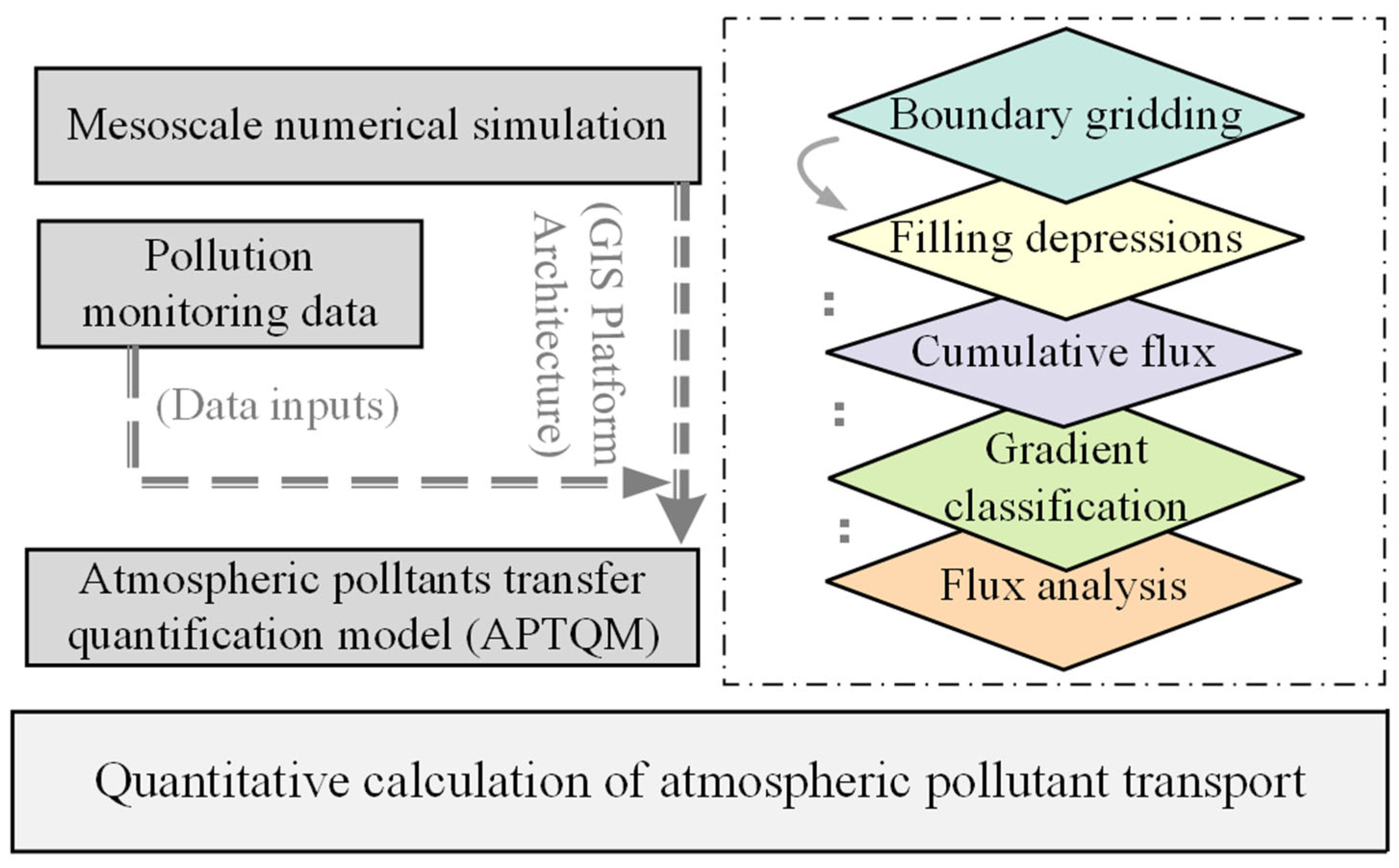
2.1. Establishment of Method

The directional movement of airflow predominantly determines the migration paths and diffusion patterns of atmospheric pollutants [26]. This study was designed to develop an efficient and accurate model for atmospheric pollutant transport quantification model (APTQM) and evaluate the contributions of inter-regional pollutant transport. Through the integration of high-resolution numerical simulation results, spatial analysis functions of Geographic Information Systems (GISs), and key statistical indicators, the patterns of pollutant transport were systematically analyzed and quantified. The model was designed with an emphasis on computational efficiency and spatial precision, thereby establishing a scientific foundation for coordinated regional pollution management. The operational framework is presented in Figure 1, wherein the workflow is categorized into four key components: high-resolution numerical simulation, pollutant transport framework establishment, transport quantification methodology, and model validation and application.

The detailed construction process is as follows:

(1)

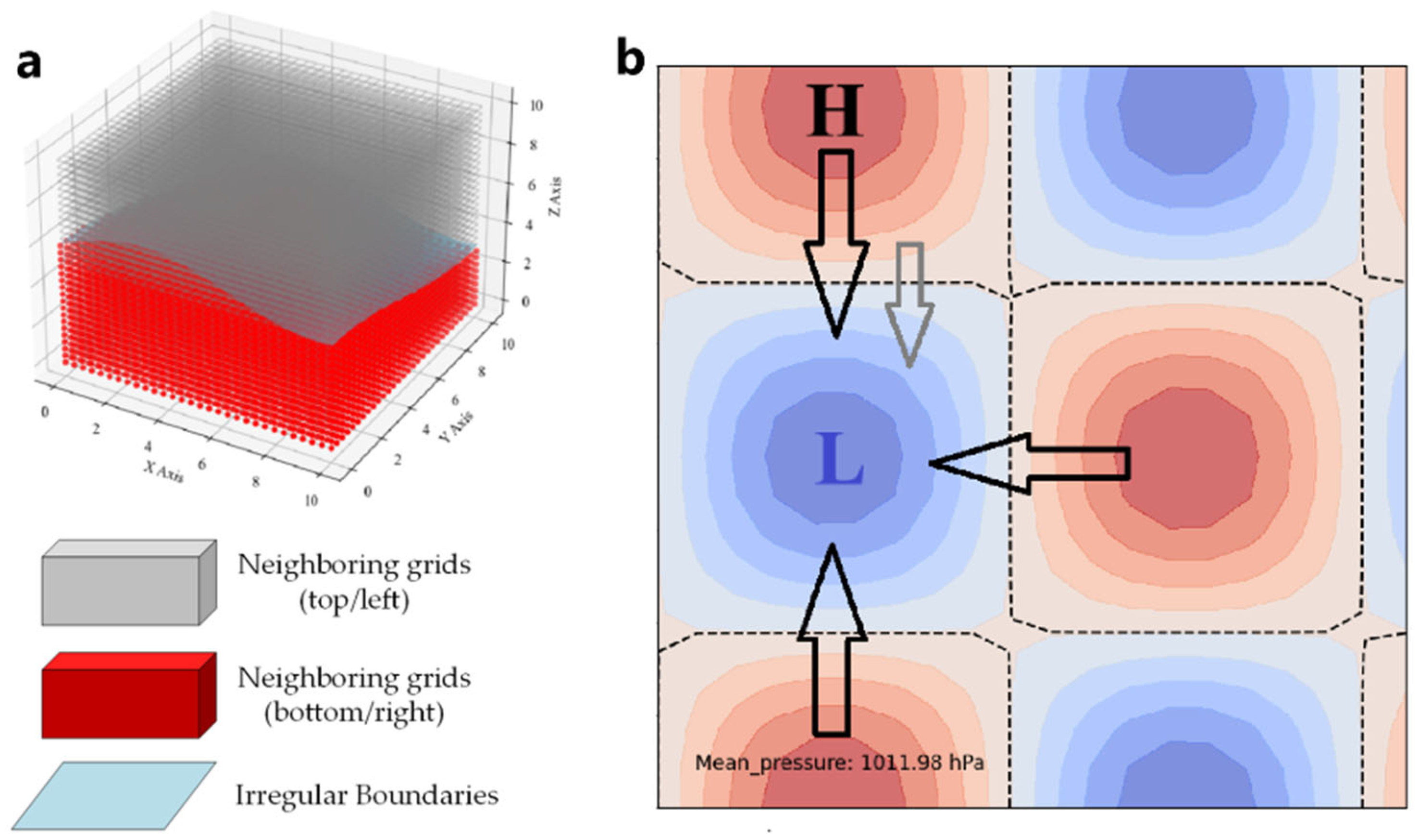
Area gridding and boundary processing

Due to the complex and irregular characteristics of study area boundaries, traditional methods are susceptible to substantial projection errors in boundary processing, thereby compromising calculation accuracy [27]. Regularized geometries have been implemented to simplify regional boundaries through multilevel mesh partitioning and an optimized numerical assignment method. Complex boundaries are transformed into regular geometries, concurrent with the decomposition of the region into 3D rectangular column grids via a hierarchical grid structure. Through this approach, boundary projection errors are significantly minimized, and grid distribution is optimized. The study area is partitioned into horizontally oriented refined grids, wherein each grid functions as a spatial unit encompassing the four directions of airflow transport. As shown in Figure 2, the actual region boundaries are simplified to fit regular grid partitions, while Figure 3a intuitively illustrates the results of grid mapping for irregular boundaries of the target region (gray wireframes indicate hierarchical grid structures). The red dots indicate the intersections of the grid and the boundary, highlighting the effectiveness of the intersection method in boundary definition.

(2)

Depression filling and pressure gradient analysis

Within atmospheric pollution transport modeling, a depression is defined as a grid characterized by an undefined transport direction and surrounded by pixels of higher values [28]. These depressions are known to cause data anomalies and computational errors, necessitating correction through pressure filling to eliminate background data defects. The pressure gradients across different regions are categorized by establishing average grid standard values to reveal detailed airflow transport processes within the region.

Grid cumulative flux, which represents the total flux received by each grid, serves as a critical indicator of atmospheric pollutant transport, characterizing both transport paths and intensities within the region. To further elucidate the dynamics of regional airflow, the pressure gradient field governs the path and intensity of airflow transport [29], while the migration path adheres to the principles of mass and energy conservation, enabling the steady-state flow energy equation to be utilized in describing the pollutant transport process under atmospheric conditions. In this study, the pressure gradient in the target region is refined into a multilevel field, which calibrates the distribution of high and low pressures and the direction of pollutant transport between different grids. The regional airflow paths are visualized using a color gradient, where high-pressure regions represent pollution sources and low-pressure regions indicate pollution sinks, as shown in Figure 3b. Red coloring denotes high-value grids, while blue coloring indicates low-value grids. The arrows represent airflow direction and strength, with black arrows indicating stronger transport and gray arrows depicting weaker transmission.

(3)

Atmospheric flow analysis and quantification methods

Atmospheric pollutant transport processes are influenced by multiple factors, including wind speed, pressure gradient, pollutant concentration, transport cross-sectional area, and buoyancy effects [30,31]. Within a stationary unit, the vertical wind field manifests as an internal ‘self-exchange’ process, while horizontal transport operates as an ‘external action’ process. The transport vector model employed herein specifically addresses the horizontal transport of pollutants.

The horizontal transport of pollutants is postulated to be governed by the regional wind field, wherein pressure data are refined through standardized grid values and cumulative flux analysis to determine specific airflow transport pathways [32]. Subsequently, grid refinement techniques are implemented to partition the target grid into nearest and second-nearest neighbors, while the pollutant grid is categorized into outflow and inflow grids (adjacent grids). To ensure compliance with physical conservation principles, the steady-state energy equation is introduced for model calibration. The steady-state energy equation is defined as follows [33]. Equations (1)–(3) are as follows:

$${\mathrm{P}}_{\alpha }+{\displaystyle \frac{{\begin{array}{c}{\rho }_1{ v}_{\alpha }\end{array}}^2}{2}}={\mathrm{P}}_{\beta }+{\displaystyle \frac{{\begin{array}{c}{\rho }_2{v}_{\beta }\end{array}}^2}{2}}+P_{\tau -2};$$

(1)

where ${\mathrm{P}}_{\alpha }$ and ${\mathrm{P}}_{\beta }$ are the absolute total pressure values (hPa) of the inflow and outflow cross-sectional surfaces, respectively; $v_{\alpha }$ is the inflow wind speed (m/s), and $v_{\beta }$ is the outflow wind speed (m/s); and $P_{\tau -2}$ is the pressure loss (hPa) of the two cross-sectional surfaces. $v$ is the airflow movement velocity of the grid, and default is the average wind speed out of the grid in m/s. Ideally, if pressure loss is not considered, the contaminated gas will flow into the tiny grid through the cross-section and then out through the cross-section. ${\rho }_1$, ${\rho }_2$ are substituted for the contaminated mass concentrations of the neighboring grids, respectively.

$${M_{\mathrm{t}}}_{\left(\sigma \right)}=v{S}_{\left(\sigma \right)}·d_t;$$

(2)

$$S_{\mathsf{\sigma }}=d_{x_{\mathsf{\sigma }}}\left(d_{y_{\mathsf{\sigma }}}\right)\ast d_{z_{\mathsf{\sigma }}}$$

(3)

${M_{\mathrm{t}}}_{\left(\sigma \right)}$ is the total transmission strength at the time period of $d_t$ in the surface of $\sigma$. $S_{\mathsf{\sigma }}$ is the cross-sectional area of the grid $\mathsf{\sigma }$ plane, $d_{x_{\mathsf{\sigma }}}$ is the length of the grid, $d_{z_{\mathsf{\sigma }}}$ is the grid height, $d_{y_{\mathsf{\sigma }}}$ is the grid width, and since the grid is already small enough, the present study assumes that all relevant physical quantities act uniformly on the grid. As shown in Figure 4, ideally, if pressure loss is not considered, the polluted gas flows into the tiny grid through section $\alpha$, and then flows out through section $\beta$. The wind speed $v_{\alpha }$ is small and the relative air pressure ${\mathrm{P}}_{\alpha }$ is low, i.e., the left side of the equation is close to 0, and the value of $v$ is negative, i.e., the pollutant transport direction of this grid is $\beta$ to $\alpha$. At this time, $M$ is negative, i.e., the pollutant at $\beta$ is inflow-dominated, and $\alpha$ is outflow-dominated, and on the contrary, $M$ is positive. Combined with the grid concentration results, Equations (4) and (5) can be modified as follows:

$${\mathrm{M}}_{{\mathrm{t}}_{\left(\mathsf{\sigma }\right)}}=\sqrt{{\displaystyle \frac{2\Delta P+{Conc}_{Trans}\ast v_1^2}{{Conc}_{receive}}}}\times S_{\mathsf{\sigma }}\times d_t;$$

(4)

$$\Delta P=\left|P_H-P_L\right|$$

(5)

where ${Conc}_{Trans}$ is the average concentration of pollutant gas in the outflow unit in ug/m³, ${Conc}_{receive}$ is the concentration of pollutant gas in the inflow unit in ug/m³, $\Delta P$ is the surface pressure difference between the outflow and inflow grids, $P_H$ is the relatively high-pressure grid, $P_L$ is the low-pressure grid in hPa, and $v_1$ is the average inflow wind speed of the grid $\mathsf{\sigma }$ surface at time $t$ (m/s).

In order to facilitate the comparison of the pollutant transport volume in each time period, the default pollutant density is the standard density of the corresponding precursor, from which the spatial horizontal transport direction of atmospheric pollutants can be judged in units of ug/m³. $d_t$ is the tiny time period in s,$d_t=T-t_0$,$t_0$ is the beginning moment (s), and $T$ is the end moment (s) in s. The transport flux ${\mathrm{T}\mathrm{r}\mathrm{a}\mathrm{n}\mathrm{s}\mathrm{M}}_{{\mathrm{t}}_{\mathsf{\sigma }}}$ for a given boundary is solved using the integral method:

$${\mathrm{T}\mathrm{r}\mathrm{a}\mathrm{n}\mathrm{s}\mathrm{M}}_{{\mathrm{t}}_{\mathsf{\sigma }}}={\iiint }_{\left(i,j,t_0\right)}{\mathrm{M}}_{{\mathrm{t}}_{\mathsf{\sigma }}}={\int }_{t0}{d}_t{\iint }_{x=x_1,y=y1}^{i,j}{\mathrm{M}}_{{\mathrm{t}}_{\mathsf{\sigma }}}$$

(6)

Here, ${\mathrm{T}\mathrm{r}\mathrm{a}\mathrm{n}\mathrm{s}\mathrm{M}}_{{\mathrm{t}}_{\mathsf{\sigma }}}$ is the cumulative transport flux of the polluted gas to the $\mathsf{\sigma }$ plane of the target grid during the $d_t$ time period in ug. It is derived from Equation (6) as a quantity of the transport flux in the four-week direction. ${\mathrm{T}\mathrm{r}\mathrm{a}\mathrm{n}\mathrm{s}\mathrm{M}}_{{\mathrm{t}}_{\mathrm{W}}}$ is the west inflow, ${\mathrm{T}\mathrm{r}\mathrm{a}\mathrm{n}\mathrm{s}\mathrm{M}}_{{\mathrm{t}}_{\mathrm{E}}}$ is the east inflow,${\mathrm{T}\mathrm{r}\mathrm{a}\mathrm{n}\mathrm{s}\mathrm{M}}_{{\mathrm{t}}_{\mathrm{N}}}$ is the north inflow, and ${\mathrm{T}\mathrm{r}\mathrm{a}\mathrm{n}\mathrm{s}\mathrm{M}}_{{\mathrm{t}}_{\mathrm{S}}}$ is the south inflow; all units are in m³.

$${\mathrm{T}\mathrm{r}\mathrm{a}\mathrm{n}\mathrm{s}\mathrm{M}}_{{\mathrm{t}}_{\mathrm{W}}}={\int }_{t0}{d}_t{\iint }_{x=x_1,y=y_1}^{i,j}{\left(2\Delta P+{Conc}_{Trans}·v_1^2+19.6\Delta {\mathrm{d}}_z/{Conc}_{receive}\right)}^{\frac{1}{2}}{ ·{Conc}_{Trans}·d}_{x_{i,j}}{d}_{z_{i,j}};$$

(7)

$${\mathrm{T}\mathrm{r}\mathrm{a}\mathrm{n}\mathrm{s}\mathrm{M}}_{{\mathrm{t}}_{\mathrm{E}}}={\int }_{t0}{d}_t{\iint }_{x=x_1,y=y_1}^{i,j}{\left(2\Delta P+{Conc}_{Trans}·v_1^2+19.6\Delta {\mathrm{d}}_z/{Conc}_{receive}\right)}^{\frac{1}{2}}{ ·{Conc}_{Trans}·d}_{x_{i,j}}{d}_{z_{i,j}};$$

(8)

$${\mathrm{T}\mathrm{r}\mathrm{a}\mathrm{n}\mathrm{s}\mathrm{M}}_{{\mathrm{t}}_{\mathrm{N}}}={\int }_{t0}{d}_t{\iint }_{x=x_1,y=y_1}^{i,j}{\left(2\Delta P+{Conc}_{Trans}·v_1^2+19.6\Delta {\mathrm{d}}_z/{Conc}_{receive}\right)}^{\frac{1}{2}}{·{Conc}_{Trans} ·d}_{y_{i,j}}{d}_{z_{i,j}} ;$$

(9)

$${\mathrm{T}\mathrm{r}\mathrm{a}\mathrm{n}\mathrm{s}\mathrm{M}}_{{\mathrm{t}}_{\mathrm{S}}}={\int }_{t0}{d}_t{\iint }_{x=x_1,y=y_1}^{i,j}{\left(2\Delta P+{Conc}_{Trans}·v_1^2+19.6\Delta {\mathrm{d}}_z/{Conc}_{receive}\right)}^{\frac{1}{2}}{·{Conc}_{Trans} ·d}_{y_{i,j}}{d}_{z_{i,j}}$$

(10)

2.2. Validation of Method

The four-dimensional (4D) flux, which is widely applied in air pollution quantification, integrates temporal, spatial, and altitudinal dimensions to enable a comprehensive assessment of pollutant transport processes. The principles of this method are systematically detailed in Liulin Yang et al.’s [34] comprehensive exposition of 4D flux. This approach allows for the analysis of horizontal diffusion in multiple directions as well as the simulation of vertical transport, making it an essential tool for examining complex air pollution events. Consequently, the method has been extensively employed to verify migration quantification results and to provide a unified framework for analyzing pollutant transport characteristics [35,36,37]. The equations governing this methodology are presented as follows:

$$\mathrm{M}=\mathrm{C}\mathrm{o}\mathrm{n}\mathrm{c}·{\mathrm{W}}_{\mathrm{S}}·\mathrm{S}·\mathrm{T}$$

(11)

where $\mathrm{M}$ is the transported flux in μg, $\mathrm{C}\mathrm{o}\mathrm{n}\mathrm{c}$ is the target pollutant concentration in ug/m³, $W_S$ is the wind speed perpendicular to the particular interface in m/s, $\mathrm{S}$ is the area of the particular interface in m², and $\mathrm{T}$ is the time in s.

While the transport quantification model (APTQM) exhibits both geometric precision and methodological robustness, comprehensive validation of its reliability is essential due to its novel nature. The feasibility and effectiveness of APTQM were evaluated through two approaches: (1) the 4D flux method for quantifying contribution magnitude, and (2) WRF-FLEXPART simulations to analyze the spatial distribution of potential source areas.

3. Application, Validation and Discussion

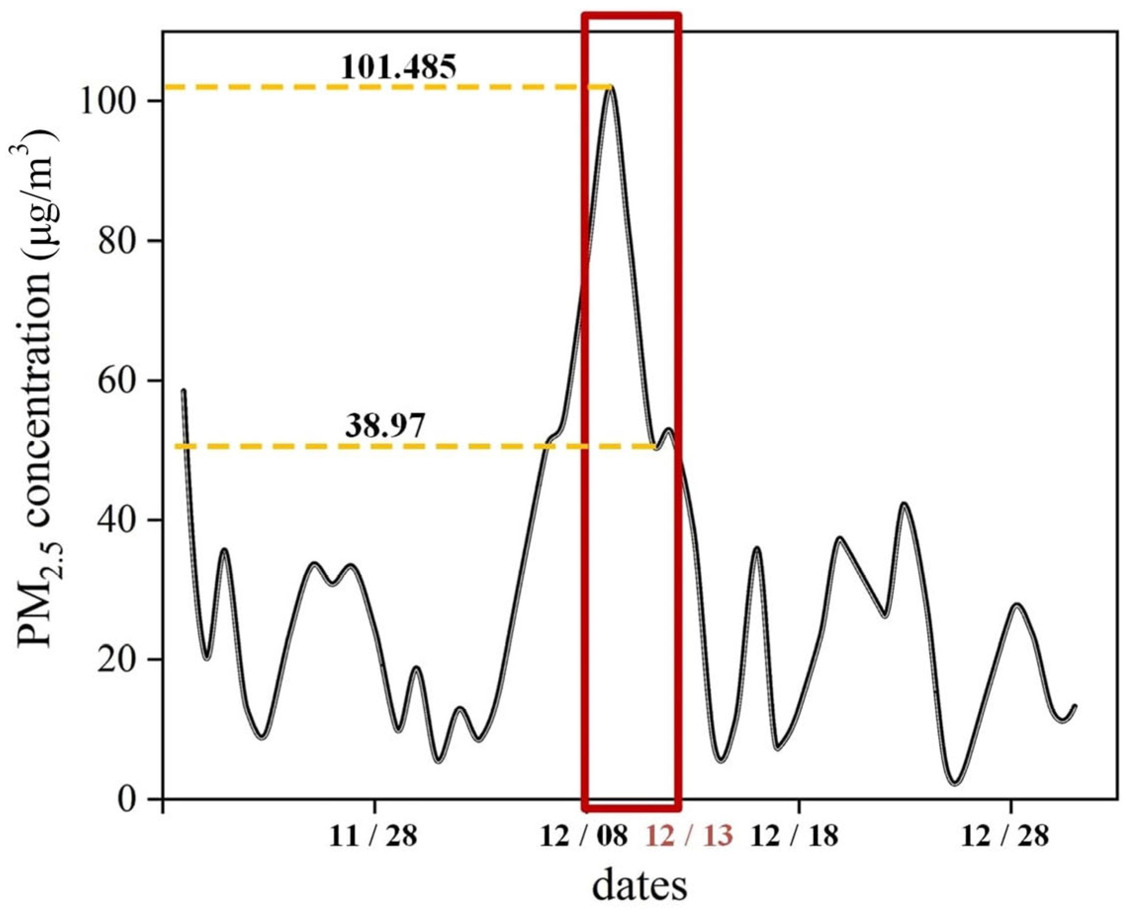
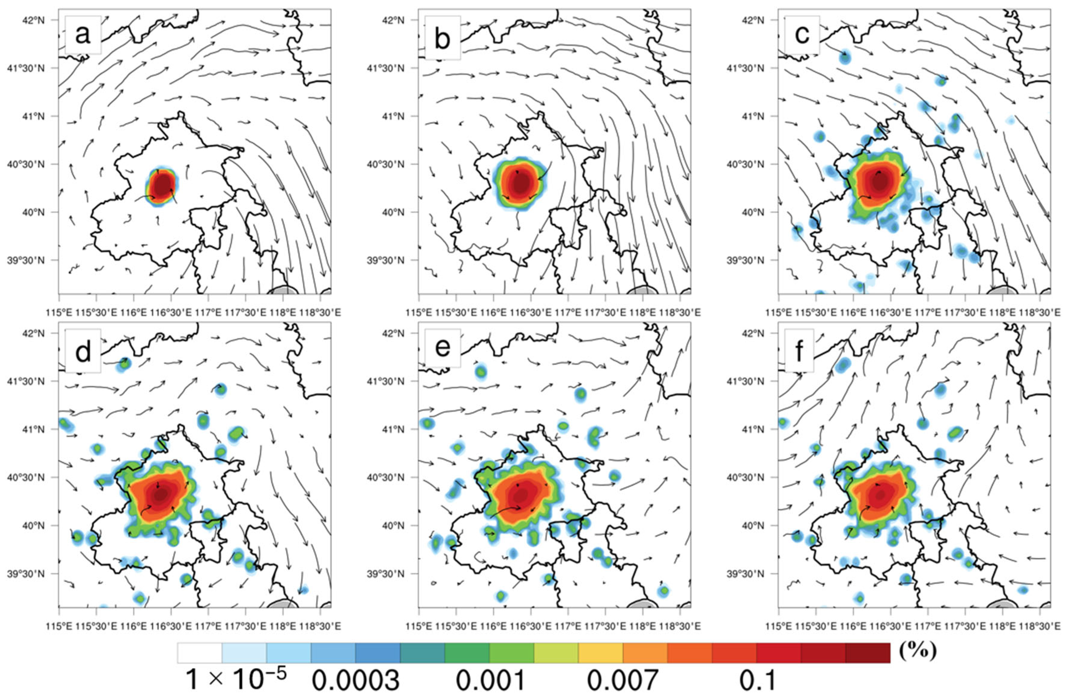
3.1. Case Selection and Numerical Simulation

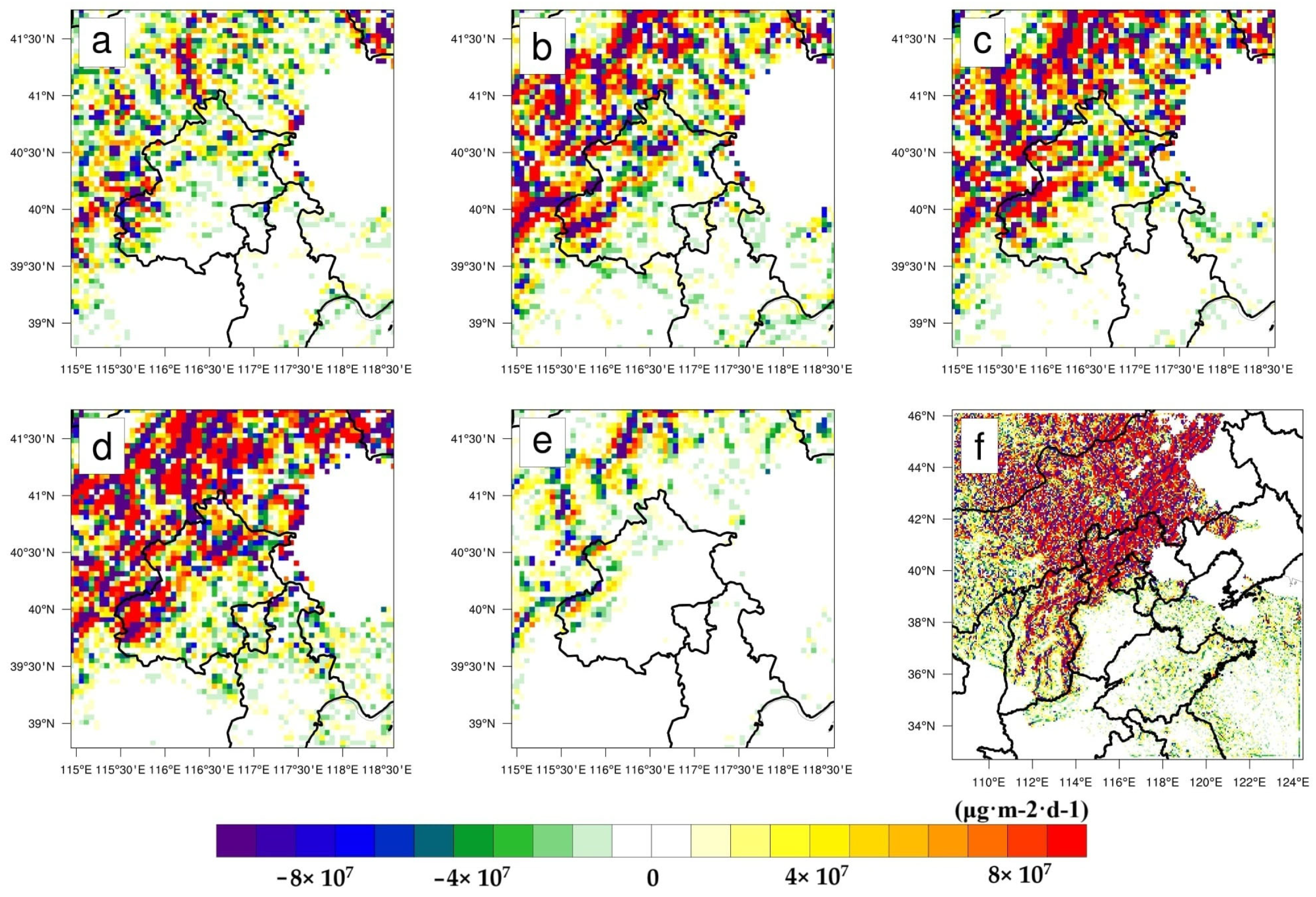
Previous studies have demonstrated that elevated PM_2.5 concentrations are frequently associated with haze events [38]. In urban air pollution, particularly in Beijing, the winter season is characterized by a higher incidence of severe air pollution, which is primarily attributed to the combination of coal-fired heating and other anthropogenic emission sources [39]. Between 8 and 13 December 2021, a significant PM_2.5 pollution event occurred in Beijing. This event took place during the winter heating season, when the North China Plain was under the influence of weak high-pressure systems, with the center of a low-pressure system located at the border between Zhangjiakou and Inner Mongolia. Beijing was positioned behind the low-pressure trough, which led to a stagnant weather pattern characterized by high humidity and low temperatures. The vertical mixing of air was significantly suppressed, causing pollutants to accumulate in the near-surface layer [40,41]. This hindered their effective dispersion and intensified the lateral transport of pollutants. In this study, the pollution event is analyzed in detail, and the previously developed transport quantification model is validated by calculating boundary fluxes and assessing the relative contributions of pollutant transport. Real-time PM_2.5 concentration data were obtained from the China-High-Air-Pollutants (CHAP) dataset, published by the National Tibetan Plateau Scientific Data Release (NTPSDR) (https://data.tpdc.ac.cn/zh-hans/data/, accessed on 4 April 2024), with a spatial resolution of 1 km and measurements in µg/m³. The monitoring data revealed that PM_2.5 concentrations peaked at 101.485 µg/m³ at 11:00 (UTC is used throughout) on 9 December, and reached a minimum of 38.97 µg/m³ at 10:00 on 12 December. A slight increase in PM_2.5 concentrations was observed on 13 December, followed by a gradual decline marking the end of the pollution episode (Figure 5).

The Weather Research and Forecasting (WRF) model is implemented as a fully compressible, non-hydrostatic mesoscale atmospheric model designed for simulating pollution processes [42]. The simulation domain was centered at 38.74° N, 114.8° E, incorporating 32 vertical layers. The simulation was conducted from 00:00 on 7 December 2021 to 00:00 on 13 December 2021 (144 h), with the initial 12 h designated as the spin-up period. As shown in Figure 6, the simulation was configured with three nested domains, of which the innermost domain was utilized for analysis, featuring a grid resolution of 5 km × 5 km. The accuracy of wind field simulation significantly influences the performance of the APTQM model. David et al. [43] performed a sensitivity study of the WRF-simulated wind speed using different physical schemes. The results indicate that the YSU scheme presents great results in wind simulations. While wind direction is relatively insensitive to parameter selection, it is highly influenced by topography. Among various schemes, the YSU scheme has demonstrated exceptional performance in simulating near-surface wind conditions [44]. Therefore, for the current study, the WSM Type 3 simple ice scheme was selected for microphysics, combined with the Monin–Obukhov surface layer scheme, YSU boundary layer scheme, Grell 3D cumulus parameterization scheme, and thermal diffusion scheme. The initial meteorological data and boundary layer conditions used are the global reanalysis data (FNL data) provided by NCEP/NCAR, USA, with a spatial resolution of 1° × 1° and a temporal resolution of 6 h (00:00, 06:00, 12:00, 18:00).

The WRF-simulated meteorological field primarily includes the simulation of four key meteorological elements: 2m-temperature (2m-T), relative humidity (RH), sea level pressure (SLP), and 10m wind speed (10m-WSPD). The observed meteorological data utilized in this study were obtained from the China Meteorological Administration’s Open Data Platform (http://www.nmic.cn/, accessed on 3 April 2024). Data from 18 monitoring stations in Beijing were grouped into four regions (Figure 7a), and the arithmetic mean of the monitoring values from all stations within each region was calculated. This regional average was used as the standard value for comparison with the WRF simulation results to evaluate the model’s performance. The orientation of each region was determined relative to the city center.

Figure 7b presents the Taylor diagram illustrating the comparison between modeled and observed values in Beijing during the pollution period. The correlation coefficients between simulated and observed air temperature and relative humidity are as high as 0.87, although slightly lower in the northern part of the city due to the absence of certain measurements. However, even in these cases, the coefficients remain above 0.6. For wind speed, the correlation coefficients between simulated and observed values exceed 0.6, and the results successfully pass the 95% significance level test. Given the critical role of the wind field in the simulation, near-surface wind field observations were compared with model simulations at 12:00 on 9–11 December for validation purposes as shown in Figure 8. The simulated wind patterns demonstrated strong agreement with observations, exhibiting consistent correlation in both wind speed and directional components. While instantaneous wind parameters exhibited deviations due to surface–layer interactions and local terrain effects, the simulation successfully captured the dominant flow patterns and their temporal evolution, particularly in the Beijing metropolitan region and its vicinity. These results validate the reliability of the simulated meteorological fields for subsequent pollutant transport and dispersion analyses. Therefore, the simulated meteorological fields can be used for the simulation and analysis of pollutant transport.

Figure 9 and

Table 1. PM_2.5 transmission at the boundary of the auxiliary calculation in Beijing (ATPQM).

Times(mm/d)	Transport Strength (μg·m−2·d−1)				Net Flux (μg·d−1)
	Eastern	Southern	Western	Northern
12/8	1.366 × 108	−1.447 × 108	−3.192 × 107	−3.23 × 107	−3.227 × 107
12/9	−3.496 × 107	−2.563 × 108	1.515 × 108	7.625 × 107	−6.346 × 107
12/10	3.433 × 108	−1.05 × 109	6.735 × 106	2.492 × 107	−6.749 × 108
12/11	3.281 × 108	−4.653 × 108	6.337 × 106	1.857 × 108	5.475 × 107
12/12	2.007 × 107	−1.323 × 108	1.597 × 106	−2.207 × 107	−1.327 × 108
Sum	8.29 × 108	−2.05 × 109	1.34 × 108	2.33 × 108	−8.49 × 108
Average	1.67 × 108	−4.10 × 108	2.68 × 107	4.65 × 107	−1.70 × 108

demonstrate that the spatial–temporal evolution of PM_2.5 net flux during the heavy pollution period exhibited distinct directional characteristics and intensity variations. The period of 8–9 December (Figure 9a,b) was characterized by moderate transport intensity, wherein negative net flux predominated in the northwestern region. Significant intensification was observed on 10 December (Figure 9c), with the southern boundary exhibiting peak outward transport (−1.05 × 10⁹ μg·m⁻²·d⁻¹) concurrent with inward transport at the eastern boundary (3.433 × 10⁸ μg·m⁻²·d⁻¹). A notable shift in transport dynamics was documented on 11 December (Figure 9d), characterized by sustained inward transport at the eastern boundary (3.281 × 10⁸ μg·m⁻²·d⁻¹) and attenuated outward transport at the southern boundary (−4.653 × 10⁸ μg·m⁻²·d⁻¹). By 12 December (Figure 9e), transport intensity was significantly reduced across all boundaries.

The five-day cumulative net flux analysis (Figure 9f) revealed several critical features:

(a)

A pronounced northwest–southeast transport corridor, evidenced by concentrated high-value regions.

(b)

Substantial negative flux at the southern boundary (mean: −4.1 × 10⁸ μg·m⁻²·d⁻¹).

(c)

Persistent positive flux at the eastern boundary (mean: 1.67 × 10⁸ μg·m⁻²·d⁻¹).

These patterns indicate two primary pollution sources: internal accumulation within Beijing’s urban area and external transport from surrounding regions. The southern boundary’s strong negative flux suggests its role as the primary pollution outlet, while the eastern boundary consistently functions as an inlet. The western and northern boundaries exhibited moderate transport intensities, with means of 2.68 × 10⁷ and 4.65 × 10⁷ μg·m⁻²·d⁻¹, respectively. The five-day total net flux of −8.49 × 10⁸ μg·d⁻¹ indicates that Beijing functioned as a net PM_2.5 exporter during this episode, although significant daily variations in transport intensity and directionality were observed. These findings suggest complex interactions among local emissions, regional transport, and meteorological conditions in determining Beijing’s PM_2.5 pollution patterns.

3.2. Validation Analysis

(1)

Quantitative comparison

A comparative analysis was performed between APTQM and the 4D flux method to evaluate their atmospheric pollutant transport capabilities (Figure 10 and

Table 2. PM_2.5 transmission at the boundary of the auxiliary calculation in Beijing (4D flux method).

Times (mm/d)	Transport Strength (μg·m−2·d−1)				Net Flux (μg·d−1)
	Eastern	Southern	Western	Northern
12/8	1.286 × 108	3.616 × 108	−3.959 × 107	−2.484 × 107	−1.112 × 107
12/9	−2.871 × 107	3.361 × 108	9.611 × 108	6.283 × 107	−6.922 × 107
12/10	2.898 × 108	−1.96 × 109	5.354 × 106	2.462 × 107	−5.847 × 108
12/11	3.4 × 108	−5.388 × 108	5.246 × 106	1.042 × 108	4.022 × 107
12/12	2.91 × 107	−1.021 × 108	1.675 × 106	−2.835 × 107	−1.963 × 108
Sum	7.95 × 108	−9.0 × 109	9.34 × 108	1.38 × 108	−8.21 × 108
Average	1.52 × 109	−3.81 × 108	1.87 × 108	2.77 × 107	−1.64 × 108

). Statistical analyses revealed strong correlation between the approaches (R² = 0.79), characterized by minimal bias and RMSE values ranging from 5 to 10%, thus demonstrating APTQM’s reliability across various transport scenarios. Quantitative assessment identified fundamental differences in transport magnitude estimation, wherein APTQM produced consistently more conservative estimates, yielding a cumulative net flux (−8.49 × 10⁸ μg·d⁻¹) approximately one order of magnitude lower than the 4D flux method (−2.51 × 10¹⁰ μg·d⁻¹). This characteristic was particularly evident in southern boundary transport, where APTQM estimates (−2.05 × 10⁹ μg·d⁻¹) indicated more moderate flux intensities compared to 4D flux (−1.31 × 10¹⁰ μg·d⁻¹), while maintaining physical consistency with overall transport patterns.

The directional transport analysis highlighted APTQM’s enhanced capacity for boundary flow representation. Notably, the eastern boundary exhibited contrasting patterns, with APTQM detecting positive transport (cumulative 8.33 × 10⁸ μg·d⁻¹) in contrast to the 4D flux method’s negative values (−7.79 × 10⁹ μg·d⁻¹). This fundamental difference suggests superior physical consistency in APTQM’s boundary flow representation, particularly in its balanced detection of multidirectional transport variations. Furthermore, APTQM demonstrated enhanced temporal resolution in capturing both internal and external transport processes. This was exemplified on December 10, where APTQM identified proportional southern (−1.05 × 10⁹ μg·d⁻¹) and eastern (3.433 × 10⁸ μg·d⁻¹) boundary transport, contrasting with the 4D flux method’s more extreme estimates (−3.96 × 10⁹ μg·d⁻¹ and −1.898 × 10⁹ μg·d⁻¹, respectively). The method’s capacity to maintain consistent boundary transport ratios while capturing significant temporal variations indicates improved reliability in representing actual transport conditions.

(2)

Analysis of Source Areas

The WRF-FLEXPART model was implemented to quantify pollution source areas and their respective contribution rates in Beijing. This model provides an efficient and accurate approach for determining the spatial–temporal distribution of air pollutant sources within the target area. The model’s output enables characterization of potential contributions from various source regions to air pollutant concentrations at specified receptor locations. The governing equations are presented as follows:

$${\mathrm{C}\mathrm{o}\mathrm{n}}_{\mathrm{r}\mathrm{a}\mathrm{t}\mathrm{e}(\mathrm{i},\mathrm{j})}={\displaystyle \frac{\begin{array}{c}{\mathrm{E}}_{(\mathrm{i},\mathrm{j})}\ast {\mathrm{r}}_{(\mathrm{i},\mathrm{j})}\end{array}}{{\sum }_{\left(\mathrm{1,1}\right)}^{(N,S)}{\mathrm{E}}_{(\mathrm{i},\mathrm{j})}\ast r_{(i,j)}}};$$

(12)

$${\mathrm{T}\mathrm{o}\mathrm{t}\mathrm{a}\mathrm{l}}_{\mathrm{r}}={\displaystyle \sum _{(N_1,S_1)}^{(N_2,S_2)}}Co{n_{rate}}_{(i,j)}$$

(13)

where $(i, j)$ is the grid location of spatial point sources; N is the total horizontal spatial grid number; N is the total vertical spatial grid number; E is the emission rate of particles; ${\mathrm{C}\mathrm{o}\mathrm{n}}_{\mathrm{r}\mathrm{a}\mathrm{t}\mathrm{e}(\mathrm{i},\mathrm{j})}$ is the grid contribution of particles; r is the grid residence time of particles; ${\mathrm{T}\mathrm{o}\mathrm{t}\mathrm{a}\mathrm{l}}_{\mathrm{r}}$ is the cumulative contribution of spatial regions; $(N_1, S_1)$ is the grid start position; and $(N_2,{ S}_2)$ is the end position.

The WRF-FLEXPART model, developed by the Norwegian Institute of Atmospheric Research (NILU), is a Linux-based Lagrangian particle diffusion model that achieved prominence in atmospheric modeling during the late 1990s and early 2000s [45,46]. The simulation was initiated on 8 December 2021, with a release duration of 4 days. Given that regional atmospheric chemistry models typically exclude metal ions, NH₃ was selected as the tracer species. To account for atmospheric particle diffusion variability and ensure uniform particle distribution across space and time, the study area was discretized into multiple grids, selecting the main city of Beijing for continuous particle release. The emission data were obtained from the Multi-resolution Emission Inventory for China (MEIC; http://www.meicmodel.org/, accessed on 23 July 2024), developed by Tsinghua University in 2016, encompassing major emission sectors including industry, electricity generation, and transportation [47]. To account for near-surface anthropogenic emission sources, a release height of 100 m above ground level was selected for the particle simulation.

Figure 11 shows the distribution of potential contribution rates and contribution rates from the WRF-FLEXPART simulation. Comparative analysis in conjunction with Figure 9 shows that the results from ATPQM and WRF-FLEXPART are in excellent agreement in both spatial and temporal dimensions. This spatial consistency was quantitatively verified through boundary flux calculations. As shown in Table 1 and Section 3.2, the APTQM results reveal significant inflow at the western boundary of Beijing during the early phase of pollution (peak: 1.515E × 10⁸ μg·m⁻²·d⁻¹ on 9 December), which aligns with the prominent easterly contribution identified by WRF-FLEXPART (Figure 11a,b). During the pollution decay period, the southern boundary exhibits the largest outflow (−1.05 × 10⁹ μg·m⁻²·d⁻¹ on 10 December), consistent with the expanded contribution region observed in the WRF-FLEXPART analysis (Figure 11c–f). The temporal evolution of transport intensity captured by APTQM effectively mirrors the dynamics of the contribution pattern identified by WRF-FLEXPART, particularly during critical transition periods.

Boundary flux analyses revealed complex transport patterns, characterized by dominant southern outflow (mean: −4.10 × 10⁸ μg·m⁻²·d⁻¹) and consistent eastern inflow (mean:1.67 × 10⁸ μg·m⁻²·d⁻¹). This directional heterogeneity aligns with WRF-FLEXPART’s spatial contribution patterns, providing additional mechanistic insights into regional pollution transport dynamics. Notably, the transition to positive net flux on 11 December (5.475 × 10⁷μg·d⁻¹) corresponds with observed changes in the FLEXPART contribution pattern and associated wind field variations. The consistent agreement between these independent methodologies validates ATPQM’s reliability as a pollution transport analysis tool.

3.3. Effects of Buoyancy

During atmospheric pollutant transport, buoyancy effects significantly influence vertical gas transport when substantial height differentials exist between adjacent cross-sections, arising from heterogeneous grid distributions. Height differentials $\Delta {\mathrm{d}}_z$ modulate gas stream trajectories and velocities via gravitational acceleration $g$. Buoyancy effects are most pronounced in vertical transport processes between elevated regions and ground level. Under buoyancy influence, less dense (warmer) air masses ascend while denser (cooler) air masses descend. To account for buoyancy influences on pollutant transport, a buoyancy parameter $\mathrm{g}\left({\mathrm{d}}_{z1}-{\mathrm{d}}_{z2}\right)$ has been incorporated into the steady-state energy equation, where grid height $\Delta {\mathrm{d}}_z$ is considered.

Therefore, the equation needs to be corrected as follows:

$${\mathrm{M}}_{{\mathrm{t}}_{\left(\mathsf{\sigma }\right)}}=\sqrt{{\displaystyle \frac{2\Delta P+{Conc}_{Trans}\ast v_1^2+19.6\Delta {\mathrm{d}}_z}{{Conc}_{receive}}}}\times S_{\mathsf{\sigma }}\times d_t$$

(14)

The buoyancy effect is quantified by a constant factor of 19.6, representing the combined influence of gravitational acceleration and air density. This parameterization enables the characterization of altitude-dependent gas transport variations. The modified ATQPM pollutant transport equation integrates three primary factors: barometric pressure gradient, wind velocity, and altitude differential. The pressure gradient drives pollutant migration from high- to low-pressure regions, while wind velocity determines transport efficiency. Additionally, the buoyancy effect significantly influences vertical pollutant transport between different altitudes.

Sensitivity analyses were performed to evaluate ATQPM performance with and without buoyancy effects, using the 4D flux method as a reference standard. In simulations excluding buoyancy, pollutant transport magnitude was significantly underestimated, particularly in highly polluted regions, resulting in insufficient vertical transport capacity and limited horizontal dispersion. The incorporation of buoyancy effects substantially enhanced peak pollutant transport and improved both vertical movement and horizontal diffusion. This enhancement was particularly evident in high-concentration zones, where thermal lifting facilitated rapid vertical transport and long-distance propagation. The modified algorithm demonstrated superior accuracy in capturing high-concentration pollution zones, especially during intense pollution events, where buoyancy effects significantly improved transport simulation fidelity.

The significance of buoyancy effects has been validated through comparative analyses of transport magnitude and pollutant dispersion patterns. While the buoyancy-inclusive algorithm demonstrates comparable performance to the 4D flux method in long-range transport simulations, it exhibits superior resolution of fine-scale pollutant dynamics, particularly during intense pollution episodes. These results establish both the theoretical validity and practical advantages of incorporating buoyancy effects, especially in simulating strong pollution events. This improved performance has been consistently demonstrated across multiple simulation scenarios, particularly in capturing detailed pollutant transport dynamics during severe pollution episodes.

4. Conclusions

The atmospheric pollutant transport quantification model (APTQM) has been developed as a novel methodological framework that synthesizes high-resolution numerical simulation, GIS capabilities, and advanced statistical indicators for quantifying cross-regional atmospheric pollutant transport. APTQM effectively addresses the limitations of traditional qualitative meteorological analyses while simultaneously reducing the computational demands inherent in comprehensive atmospheric chemistry models, thereby enabling efficient assessment of pollutant transport mechanisms and source contributions across multiple spatial and temporal scales.

Validation studies have demonstrated APTQM’s robust performance through strong temporal and spatial correlation with established four-dimensional flux methods and WRF-FLEXPART source contribution analyses. Despite minor numerical magnitude variations, comprehensive comparative analyses have confirmed APTQM’s practical utility and reliability in transport quantification. A distinctive feature of APTQM lies in its ability to capture balanced transport patterns while maintaining physical consistency across boundaries, as evidenced by coherent daily variability and boundary-specific transport signatures. The model’s ability to resolve both internal and external transport processes, along with stable transmission amplitude patterns exhibiting symmetric deviation distributions, makes it a reliable tool for studying the inter-regional interactions of air pollution.

The framework enables resolution of multidirectional transfer processes while maintaining computational efficiency. However, several methodological uncertainties warrant consideration, particularly regarding parameter optimization, including pollutant emission intensity and boundary transport conditions. These parameters necessitate careful calibration specific to study objectives to enhance model accuracy and applicability. Notwithstanding these considerations, APTQM represents a significant advancement in atmospheric transport quantification, offering an optimal balance between computational efficiency and analytical depth while maintaining robust physical consistency in transport pattern analysis.

References

1. Yan, F.; Chen, W.; Jia, S.; Zhong, B.; Yang, L.; Mao, J.; Chang, M.; Shao, M.; Yuan, B.; Situ, S.; et al. Stabilization for the secondary species contribution to PM2.5 in the Pearl River Delta (PRD) over the past decade, China: A meta-analysis. Atmos. Environ. 2020, 242, 117817. [Google Scholar] [CrossRef]
2. Liu, Y.; Wang, H.; Jing, S.; Peng, Y.; Gao, Y.; Yan, R.; Wang, Q.; Lou, S.; Cheng, T.; Huang, C. Strong regional transport of volatile organic compounds (VOCs) during wintertime in Shanghai megacity of China. Atmos. Environ. 2021, 244, 117940. [Google Scholar] [CrossRef]
3. Kumar, P.; Hama, S.; Omidvarborna, H.; Sharma, A.; Sahani, J.; Abhijith, K.; Debele, S.E.; Zavala-Reyes, J.C.; Barwise, Y.; Tiwari, A. Temporary reduction in fine particulate matter due to ‘anthropogenic emissions switch-off’ during COVID-19 lockdown in Indian cities. Sustain. Cities Soc. 2020, 62, 102382. [Google Scholar] [CrossRef] [PubMed]
4. Jiang, L.; He, S.; Zhou, H. Spatio-temporal characteristics and convergence trends of PM2.5 pollution: A case study of cities of air pollution transmission channel in Beijing-Tianjin-Hebei region, China. J. Clean. Prod. 2020, 256, 120631. [Google Scholar] [CrossRef]
5. Jeong, Y.-C.; Yeh, S.-W.; Jeong, J.I.; Park, R.J.; Yoo, C.; Yoon, J.-H. Intrinsic atmospheric circulation patterns associated with high PM2.5 concentration days in South Korea during the cold season. Sci. Total Environ. 2023, 863, 160878. [Google Scholar] [CrossRef]
6. Gu, S.; Wu, S.; Yang, L.; Hu, Y.; Tian, B.; Yu, Y.; Ma, N.; Ji, P.; Zhang, B. Synoptic Weather Patterns and Atmospheric Circulation Types of PM2.5 Pollution Periods in the Beijing-Tianjin-Hebei Region. Atmosphere 2023, 14, 942. [Google Scholar] [CrossRef]
7. Lu, D.; Mao, W.; Xiao, W.; Zhang, L. Non-Linear Response of PM2.5 Pollution to Land Use Change in China. Remote Sens. 2021, 13, 1612. [Google Scholar] [CrossRef]
8. Wu, Y.; Liu, J.; Zhai, J.; Cong, L.; Wang, Y.; Ma, W.; Zhang, Z.; Li, C. Comparison of dry and wet deposition of particulate matter in near-surface waters during summer. PLoS ONE 2018, 13, e0199241. [Google Scholar] [CrossRef]
9. Zhang, J.-D.; Cheng, X.-F.; He, Y.-T.; Kong, L.-S.; Chen, D.; Zhang, Y.-L.; Li, B. Environmental pollution, trade openness and the health of middle-aged and elderly people: An analysis of threshold effect based on data from 111 prefecture-level cities in China. Arch. Public Health 2024, 82, 202. [Google Scholar] [CrossRef]
10. Yuan, X.; Li, H.; Zhao, J. Impact of Environmental Pollution on Health-Evidence from Cities in China. Soc. Work Public Health 2020, 35, 413–430. [Google Scholar]
11. Xu, M.; Qin, Z.; Zhang, S.; Xie, Y. Health and economic benefits of clean air policies in China: A case study for Beijing-Tianjin-Hebei region. Environ. Pollut. 2021, 285, 117525. [Google Scholar] [CrossRef] [PubMed]
12. Zeng, Y.; Zhang, J.; Li, D.; Liao, Z.; Bian, J.; Bai, Z.; Shi, H.; Xuan, Y.; Yao, Z.; Chen, H. Vertical distribution of tropospheric ozone and its sources of precursors over Beijing: Results from ~20 years of ozonesonde measurements based on clustering analysis. Atmos. Res. 2023, 284, 106610. [Google Scholar] [CrossRef]
13. Zhang, C.; Lu, M.; Ma, N.; Yang, Y.; Wang, Y.; Größ, J.; Fan, Z.; Wang, M.; Wiedensohler, A. Hygroscopicity of aerosol particles composed of surfactant SDS and its internal mixture with ammonium sulfate at relative humidities up to 99.9%. Atmos. Environ. 2023, 298, 119625. [Google Scholar] [CrossRef]
14. Lu, Y.; Wang, R.; Shi, Y.; Su, C.; Yuan, J.; Johnson, A.C.; Jenkins, A.; Ferrier, R.C.; Chen, D.; Tian, H.; et al. Interaction between pollution and climate change augments ecological risk to a coastal ecosystem. Ecosyst. Health Sustain. 2018, 4, 161–168. [Google Scholar] [CrossRef]
15. Actions on Air Quality: A Global Summary of Policies and Programmes to Reduce Air Pollution. Available online: https://www.unep.org/resources/report/actions-air-quality-global-summary-policies-and-programmes-reduce-air-pollution (accessed on 9 January 2025).
16. Ambient (outdoor) air pollution. Available online: https://www.who.int/news-room/fact-sheets/detail/ambient-(outdoor)-air-quality-and-health (accessed on 9 January 2025).
17. Streets, D.G.; Fu, J.S.; Jang, C.J.; Hao, J.; He, K.; Tang, X.; Zhang, Y.; Wang, Z.; Li, Z.; Zhang, Q.; et al. Air quality during the 2008 Beijing Olympic Games. Atmos. Environ. 2007, 41, 480–492. [Google Scholar] [CrossRef]
18. Barman, N.; Gokhale, S. Transported aerosols regulate the pre-monsoon rainfall over north-east India: A WRF-Chem modelling study. Atmos. Chem. Phys. 2023, 23, 6197–6215. [Google Scholar] [CrossRef]
19. Shulan, W.; Yuanhang, Z.; Liuju, Z.; Jinlong, L.; Qun, Y. Interaction of Air Pollution among Cities in the Pearl River Delta Region. China Environ. Sci. 2005, 25, 133–137. [Google Scholar]
20. Meiyuan, H.; Zifa, W.; Dongyang, H.; Huaying, X.; Ling, Z. Modeling studies on sulfur deposition and transport in East Asia. Water Air Soil Pollut. 1995, 85, 1921–1926. [Google Scholar] [CrossRef]
21. Shikhovtsev, M.Y.; Obolkin, V.A.; Khodzher, T.V.; Molozhnikova, Y.V. Variability of the Ground Concentration of Particulate Matter PM1–PM10 in the Air Basin of the Southern Baikal Region. Atmos. Ocean. Opt. 2024, 36, 655–662. [Google Scholar]
22. Nathan, B.; Kremser, S.; Mikaloff-Fletcher, S.; Bodeker, G.; Bird, L.; Dale, E.; Lin, D.; Olivares, G.; Somervell, E. The MAPM (Mapping Air Pollution eMissions) method for inferring particulate matter emissions maps at city scale from in situ concentration measurements: Description and demonstration of capability. Atmos. Chem. Phys. 2021, 21, 14089–14108. [Google Scholar] [CrossRef]
23. Kaldellis, J.; Chalvatzis, K.; Spyropoulos, G. Chalvatzis and G.C. Spyropoulos, Transboundary air pollution balance in the new integrated European environment. Environ. Sci. Policy 2007, 10, 725–733. [Google Scholar] [CrossRef]
24. Yan, W. Analysis on the Characteristics of Horizontal Transport of the Atmospheric Pollutant over the Yangtze Delta. Res. Environ. Sci. 2008, 21, 22–29. [Google Scholar]
25. Zifa, W. Simulation of the Impacts of Regional Transport on Summer Ozone Levels Over Beijing. Chin. J. Nat. 2008, 30, 194–198. [Google Scholar]
26. Lim, E.; Chung, J.; Sandberg, M.; Ito, K. Influence of chemical reactions and turbulent diffusion on the formation of local pollutant concentration distributions. Build. Environ. 2020, 168, 106487. [Google Scholar] [CrossRef]
27. Zhu, M.; Song, Y.H.; Uhm, K.-B.; Turner, R.W.; Lee, J.-H.; Roderick, G.K. Simulation of the Long Range Migration of Brown Planthopper, Nilaparvata lugens (Stal), by Using Boundary Layer Atmospheric Model and the Geographic Information System. J. Asia-Pac. Entomol. 2000, 3, 25–32. [Google Scholar] [CrossRef]
28. Wanghe, K.; Guo, X.; Ahmad, S.; Tian, F.; Nabi, G.; Strelnikov, I.I.; Li, K.; Zhao, K. FRESF model: An ArcGIS toolbox for rapid assessment of the supply, demand, and flow of flood regulation ecosystem services. Ecol. Indic. 2022, 143, 109264. [Google Scholar] [CrossRef]
29. Bal, M.; Dandpat, A.K.; Naik, B. Hydrological modeling with respect to impact of land-use and land-cover change on the runoff dynamics in Budhabalanga river basing using ArcGIS and SWAT model. Remote Sens. Appl. Soc. Environ. 2021, 23, 100527. [Google Scholar] [CrossRef]
30. Zhang, H.; Xu, T.; Wang, Y.; Zong, Y.; Li, S.; Tang, H. Study on the influence of meteorological conditions and the street side buildings on the pollutant dispersion in the street canyon. Build. Simul. 2016, 9, 717–727. [Google Scholar] [CrossRef]
31. Yan, L.; Hu, W.; Yin, M.-Q. An Investigation of the Correlation between Pollutant Dispersion and Wind Environment: Evaluation of Static Wind Speed. Pol. J. Environ. Stud. 2021, 30, 4311–4323. [Google Scholar] [CrossRef]
32. Sun, J.L. Incorporating the Work Done by Vertical Density Fluxes in Both Kinetic and Thermal Energy Conservation Equations to Satisfy Total Energy Conservation. J. Appl. Meteorol. Climatol. 2019, 58, 213–230. [Google Scholar] [CrossRef]
33. McNaughton, K.G. The Flow of Mechanical Energy in Convective Boundary Layers. Bound. Layer Meteorol. 2012, 145, 145–163. [Google Scholar] [CrossRef]
34. Yang, L.; Wang, X.; Chen, Q. New method for investigating regional interactions of air pollutants. Acta Sci. Circumstantiae 2012, 32, 528–536. [Google Scholar]
35. Mao, J.; Zhou, L.; Chen, W.; Wu, L.; Wang, X. Application of four-dimensional flux method in PM2.5 regional transport in the Pearl River Delta during the autumn season. China Sci. 2019, 14, 85–91+97. [Google Scholar]
36. Wu, L.P.; Mo, H.H.; Yang, L.T.; Cai, Z.J.; Wu, G.T.; Bai, Y.J.; Deng, S.X.; Situ, S.P.; Chang, M.; Wang, X.M. Quantification of Ozone Pollution Transport Based on Four-dimensional Flux Method in Foshan, China. Environ. Sci. 2023, 44, 4262–4270. [Google Scholar]
37. Gang, T.; Yuhu, H.; Gang, L. Establishment and Application of Four-dimensional Fluxes Emission Factor Model for Construction Fugitive Dust. Environ. Sci. 2009, 30, 1003–1007. [Google Scholar]
38. Li, C.; Li, F.; Cheng, Q.; Guo, Y.; Zhang, Z.; Liu, X.; Qu, Y.; An, J.; Liu, Y.; Zhang, S. Divergent summertime surface O3 pollution formation mechanisms in two typical Chinese cities in the Beijing-Tianjin-Hebei region and Fenwei Plain. Sci. Total Environ. 2023, 870, 161868. [Google Scholar] [CrossRef]
39. Cao, Q.; Yan, X.; Liu, S.; Yu, J.; Chen, S.; Zhang, Y. Temperature and phase evolution and density distribution in cross section and sound evolution during the release of dense CO2 from a large-scale pipeline. Int. J. Greenh. Gas Control 2020, 96, 103011. [Google Scholar] [CrossRef]
40. Hu, T.; Yoshie, R. Effect of atmospheric stability on air pollutant concentration and its generalization for real and idealized urban block models based on field observation data and wind tunnel experiments. J. Wind Eng. Ind. Aerodyn. 2020, 207, 104380. [Google Scholar] [CrossRef]
41. Chen, Z.; Chen, D.; Zhao, C.; Kwan, M.-P.; Cai, J.; Zhuang, Y.; Zhao, B.; Wang, X.; Chen, B.; Yang, J.; et al. Influence of meteorological conditions on PM2.5 concentrations across China: A review of methodology and mechanism. Environ. Int. 2020, 139, 105558. [Google Scholar] [CrossRef]
42. Gao, S.; Zhu, S.; Yu, H. Dynamical downscaling of temperature extremes over China using the WRF model driven by different lateral boundary conditions. Atmos. Res. 2022, 278, 106348. [Google Scholar] [CrossRef]
43. Carvalho, D.; Rocha, A.; Gómez-Gesteira, M.; Santos, C. A sensitivity study of the WRF model in wind simulation for an area of high wind energy. Environ. Model. Softw. 2012, 33, 23–34. [Google Scholar] [CrossRef]
44. Tuy, S.; Lee, H.S.; Chreng, K. Offshore wind resource mapping in Cambodia: Sensitivity assessment of the weather research and forecasting model. Energy Rep. 2022, 8, 359–364. [Google Scholar] [CrossRef]
45. Stohl, A.; Wotawa, G.; Seibert, P.; Kromp-Kolb, H. Interpolation Errors in Wind Fields as a Function of Spatial and Temporal Resolution and Their Impact on Different Types of Kinematic Trajectories. J. Appl. Meteorol. Climatol. 1995, 34, 2149–2165. [Google Scholar] [CrossRef]
46. Stohl, A.; Seibert, P. Accuracy of trajectories as determined from the conservation of meteorological tracers. Q. J. R. Meteorol. Soc. 1998, 124, 1465–1484. [Google Scholar] [CrossRef]
47. Xu, J.; Zhang, Z.; Zhao, X.; Cheng, S. Downward trend of NO2 in the urban areas of Beijing-Tianjin-Hebei region from 2014 to 2020: Comparison of satellite retrievals, ground observations, and emission inventories. Atmos. Environ. 2023, 295, 119531. [Google Scholar] [CrossRef]
Figure 1. Operational framework for atmospheric pollutant transport quantification model (APTQM).
Atmosphere 16 00163 g001
Figure 2. Simplification of the actual boundary and illustration of the grid division. (a) Actual irregular boundary; (b) simplification of boundaries; (c) border gridding.
Atmosphere 16 00163 g002
Figure 3. Grid mapping and regional airflow analysis. (a) Three-dimensional representation of hierarchical grid structures with irregular boundary mapping; (b) spatial distribution of pressure gradients and associated airflow patterns.
Atmosphere 16 00163 g003
Figure 4. (A) Conceptual diagram of unit-level transport model construction and (B) schematic diagram of cross-unit flow of atmospheric pollutants. Blue grids are relatively low values, oranges are high values.
Atmosphere 16 00163 g004
Figure 5. Temporal variations in PM2.5 concentrations observed in Beijing during 8–13 December 2021.
Atmosphere 16 00163 g005
Figure 6. WRF nested domain and study area profiles. (a) The WRF nested domain setting; (b) the topography of Beijing; (c) the spatial location and extent of Beijing.
Atmosphere 16 00163 g006
Figure 7. Beijing city area division and simulated meteorological element validation of the Taylor diagram. (a) is a schematic illustration of the regional division of Beijing for the northwest (yanqing and changping), northeast (shandianzi, miyun, huairou, and pinggu), southwest (zhaitang, xiayunling, mentougou, haidian, fengtai, and fangshan), and southeast (shunyi, chaoyang, beijing, daxing and tongzhou); (b) is a simulation-observation Taylor diagram, where azimuth denotes the correlation coefficient and radius denotes the standard deviation ratio between simulation and observation.
Atmosphere 16 00163 g007
Figure 8. Comparison of near-surface simulated and observed wind speeds and directions on 9 (a), 10 (b) and 11 (c) December at 12:00 (UTC) (black arrows are simulated values, and red indicates the major deviations of the observed values from the simulated values).
Atmosphere 16 00163 g008
Figure 9. Migration volume per unit grid (5 km × 5 km) and regional transmission distribution. (af): 8–13 December.
Atmosphere 16 00163 g009
Figure 10. Validation of simulated values of ATPQM by comparing with the 4D flux method. (a) The comparison of grid quantification results between ATPQM and 4D flux methods. (b) The histogram of the relative bias (rBias) of the ATPQM values. (c) The histogram of the relative root-mean-square error (rRMSE) for ATPQM-simulated values.
Atmosphere 16 00163 g010
Figure 11. Potential contribution from WRF-FLEXPART simulation for the unit grid (6 km × 6 km) from 8 to 13 December (af), where the filled in colors are the results of the contribution calculations.
Atmosphere 16 00163 g011