Abstract
High-quality observational datasets are essential for climate research and models, but validating and filtering decades of meteorological measurements is an enormous task. Advances in machine learning provide opportunities to expedite and improve quality control while offering insight into non-linear interactions between the meteorological variables. The Cabauw Experimental Site for Atmospheric Research in the Netherlands, known for its 213 m observation mast, has provided in situ observations for over 50 years. Despite high-quality instrumentation, measurement errors or non-representative data are inevitable. We explore machine-learning-assisted quality control, focusing on wind vane stalling at 10 m height. Wind vane stalling is treated as a binary classification problem as we evaluate five supervised methods (Logistic Regression, K-Nearest Neighbour, Random Forest, Gaussian Naive Bayes, Support Vector Machine) and one semi-supervised method (One-Class Support Vector Machine). Our analysis determines that wind vane stalling occurred 4.54% of the time annually over 20 years, often during stably stratified nocturnal conditions. The K-Nearest Neighbour and Random Forest methods performed the best, identifying stalling with approximately 75% accuracy, while others were more affected by data imbalance (more non-stalling than stalling data points). The semi-supervised method, avoiding the effects of the inherent data imbalance, also yielded promising results towards advancing data quality assurance.
1. Introduction
Monitoring and predicting the weather is a cornerstone of human existence. We have witnessed remarkable technological advances over the millennia, and yet the urgency of anthropogenic climate change demands more knowledge and certainty than ever before. Particularly over the last century, the development of computational techniques, such as numerical weather prediction, machine-learning methods, and artificial intelligence, has enhanced weather forecasting. Even so, these techniques are still fundamentally reliant on precise meteorological observations [1,2,3]. In situ observations are used to initiate, validate, and improve weather models, while still providing an empirical foundation from which we can directly investigate and understand the physics involved.
The Cabauw Experimental Site for Atmospheric Research in the Netherlands (hereafter referred to as Cabauw) maintains an extensive legacy of in situ observations. Operated by the Royal Netherlands Meteorological Institute (KNMI), continuous real-time meteorological and air quality observations have been recorded at this site since 1972. These observations are used world-wide by the scientific community to advance our understanding of surface–atmosphere interactions [4,5,6,7]. Distinctly, this site provides novel vertical profiles of fundamental meteorological variables (e.g., temperature, wind speed/direction, and visibility) which are observed along a 213 m tall mast (refer to Figure 1). Cabauw has hosted numerous scientific campaigns and has conducted extensive experiments on air quality, surface energy balance, and remote sensing over the decades (i.e., https://ruisdael-observatory.nl/ (accessed on 6 January 2025)). Despite the professional-grade instrumentation and high temporal sampling, measurement errors inevitably occur. Therefore, quality control is required to ensure that data are reported accurately before use. Currently, experts perform data validation primarily through manual processes, although some automatic checks are being developed and implemented. A critical challenge in quality control is detecting and interpreting complex meteorological phenomenon which generate atypical values across diverse instruments. Given the extensive quantity and use of Cabauw data, accurate and uniform quality control is a high priority for the KNMI. This study explores whether or not the application of machine-learning-assisted quality control to the in situ meteorological observations can benefit or support this initiative.
Until now, machine-learning applications in meteorology have been primarily focused on understanding relationships within large volumes of temporal and spatial data, as well as on forecasting applications [8]. Advances in machine learning have supported the extension of observational records and contributed to improvements in the performance of numerical and climatological models [9]. While considerable focus has been placed on predicting future meteorological conditions, machine learning also offers the potential to improve long-term observational datasets. In the context of data processing, advancements in predicting accurate meteorological values can further enhance gap-filling methodologies as well [10,11]. The application of machine learning towards the quality control of observational data is developing but remains niche, for example, in agriculture and astronomy [12,13]. Often, the machine-learning methods are developed and tailored to certain tasks where outlier detection and cross-comparison techniques are effective means for quality control. However, beyond identifying observational events of interest, machine learning also has the potential to enhance data quality assurance by providing deeper insight into the complex and interconnected meteorological phenomena, enabling more tailored and effective filtering and processing based on the meteorological conditions. Nonetheless, machine-learning-assisted quality control of meteorological observations represents a relatively unexplored area of study. Therefore, we aim to explore the potential of incorporating data-driven machine-learning methods at Cabauw to enhance the quality assessment of the in situ observations while simultaneously gaining insights into the conditions underlying the data issue.
We selected the wind direction observations at Cabauw for this analysis because these data present an interesting case study, as described in Section 2. For instance, when the reported wind direction remains unchanged, the situation is unclear: Is the wind direction exceptionally steady? Is the wind vane stalling, stuck, malfunctioning, or perhaps broken? The accompanying meteorological conditions observed can provide insight into the situation and surrounding phenomena. The intricate non-linear interplay of the local-to-large-scale meteorological variables, and the uncertainties involved, necessitates the development of novel methodologies to address and improve the assessment of this potential data issue. Specifically, our research explores two machine-learning methods: supervised machine learning (five multi-class methods) and semi-supervised machine learning (one one-class method). However, in order to implement these methods, we must first manually assess the scope and potential (meteorological) drivers involved while also effectively addressing the inherent data imbalance (more non-stalling than stalling data points). This case study provides an opportunity to examine these methodologies and gain insight into machine-learning pathways that can improve data quality control for this and similar meteorological data challenges.
To this end, we focus on the potential of machine learning to identify and shed light on wind vane stalling measured at 10 m above the surface within the past 22 years at the Cabauw site. First, we provide an overview of the Cabauw site and wind vane stalling case study in Section 2. Next, the relevant data and (machine-learning) methods are detailed in Section 3. A general analysis of wind vane stalling and the surrounding meteorological conditions is presented in the results in Section 4, prior to evaluating the performance and applicability of machine-learning-assisted quality control to such datasets. Finally, Section 5 summarises the main findings and discusses the future implications of this work in assuring data quality at observational sites like Cabauw.

Figure 1.
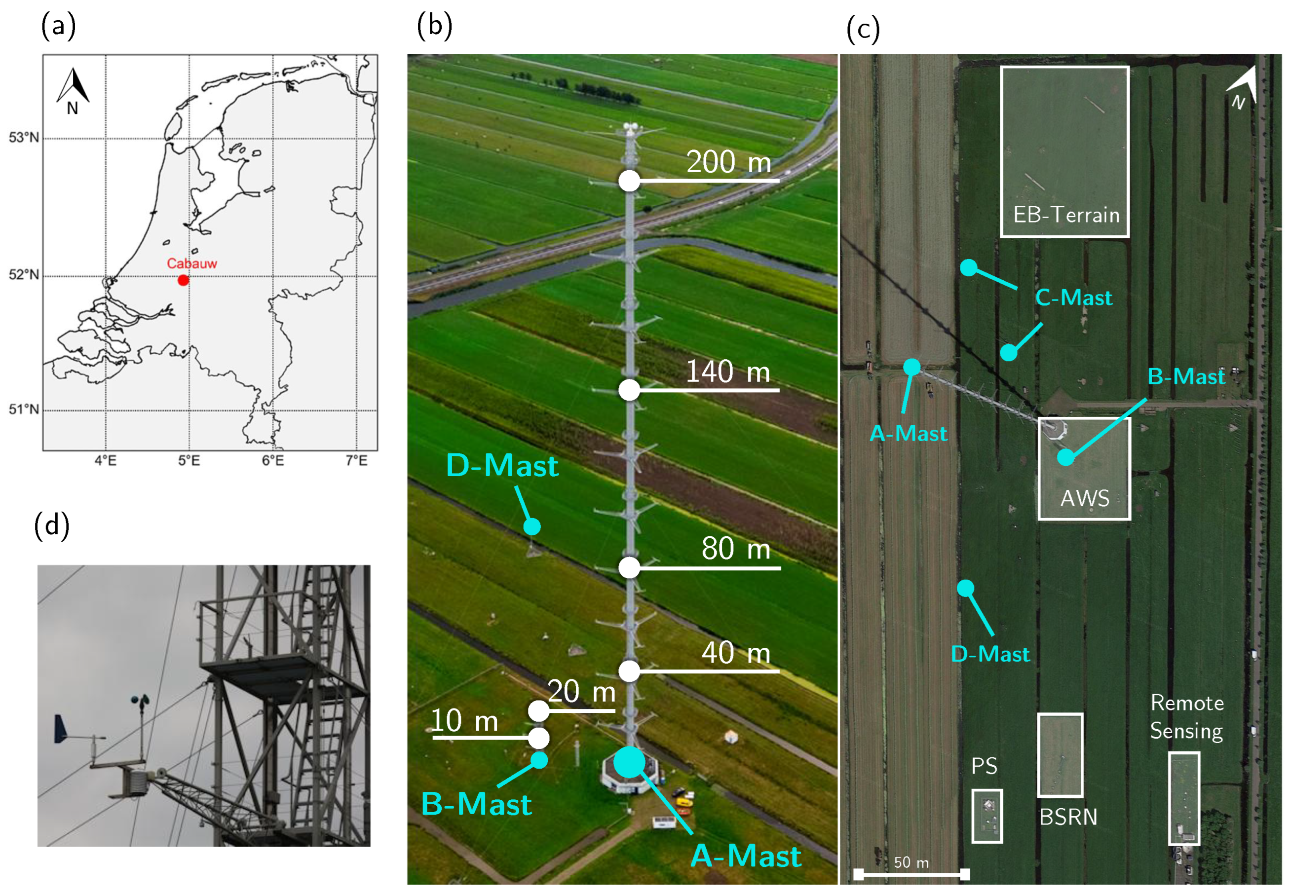
Overview of the Cabauw Experimental Site for Atmospheric Research, located in Lopik, the Netherlands. (a) Map indicating location of Cabauw site, courtesy of Knoop et al. 2021 [14]. (b) Side-view of the A-mast (main tower) indicating the levels where measurements are conducted: 10, 20, 40, 80, 140, and 200 m. (c) Top-view of sub-sites: Baseline Surface Radiation (BSRN), Profiling Site (PS), Automatic Weather Station (AWS), Energy Balance (EB) terrain, and Remote Sensing. Satellite imagery sourced from Google Earth. (d) Photo of the installed KNMI-manufactured wind vane and cup anemometer combination.
Figure 1.
Overview of the Cabauw Experimental Site for Atmospheric Research, located in Lopik, the Netherlands. (a) Map indicating location of Cabauw site, courtesy of Knoop et al. 2021 [14]. (b) Side-view of the A-mast (main tower) indicating the levels where measurements are conducted: 10, 20, 40, 80, 140, and 200 m. (c) Top-view of sub-sites: Baseline Surface Radiation (BSRN), Profiling Site (PS), Automatic Weather Station (AWS), Energy Balance (EB) terrain, and Remote Sensing. Satellite imagery sourced from Google Earth. (d) Photo of the installed KNMI-manufactured wind vane and cup anemometer combination.
2. Wind Vane Stalling
Wind direction and speed are measured at the Cabauw site with a KNMI-manufactured cup-anemometer and wind vane combination (Figure 1d), which are installed according to World Meteorological Organization (WMO) standards [15]. Wind measurements at 10 and 20 m are recorded along the B-mast, adjacent to the A-mast, in order to avoid the influence of the main tower’s base. Above the base, wind observations are measured along the A-mast at four heights: 40, 80, 140, and 200 m (Figure 1b). To avoid measuring flow disturbed by the tower itself, two cup-anemometers and three wind vanes are installed at each level. The three booms holding these instruments are oriented towards 0°, 120°, and 240° due north. Additional details can be found in Bosveld et al. 2020 [16]. At each height, the combined reported wind speed and direction ensures an accurate reading at all times. Nonetheless, issues will arise, compromising the accuracy of these measurements.
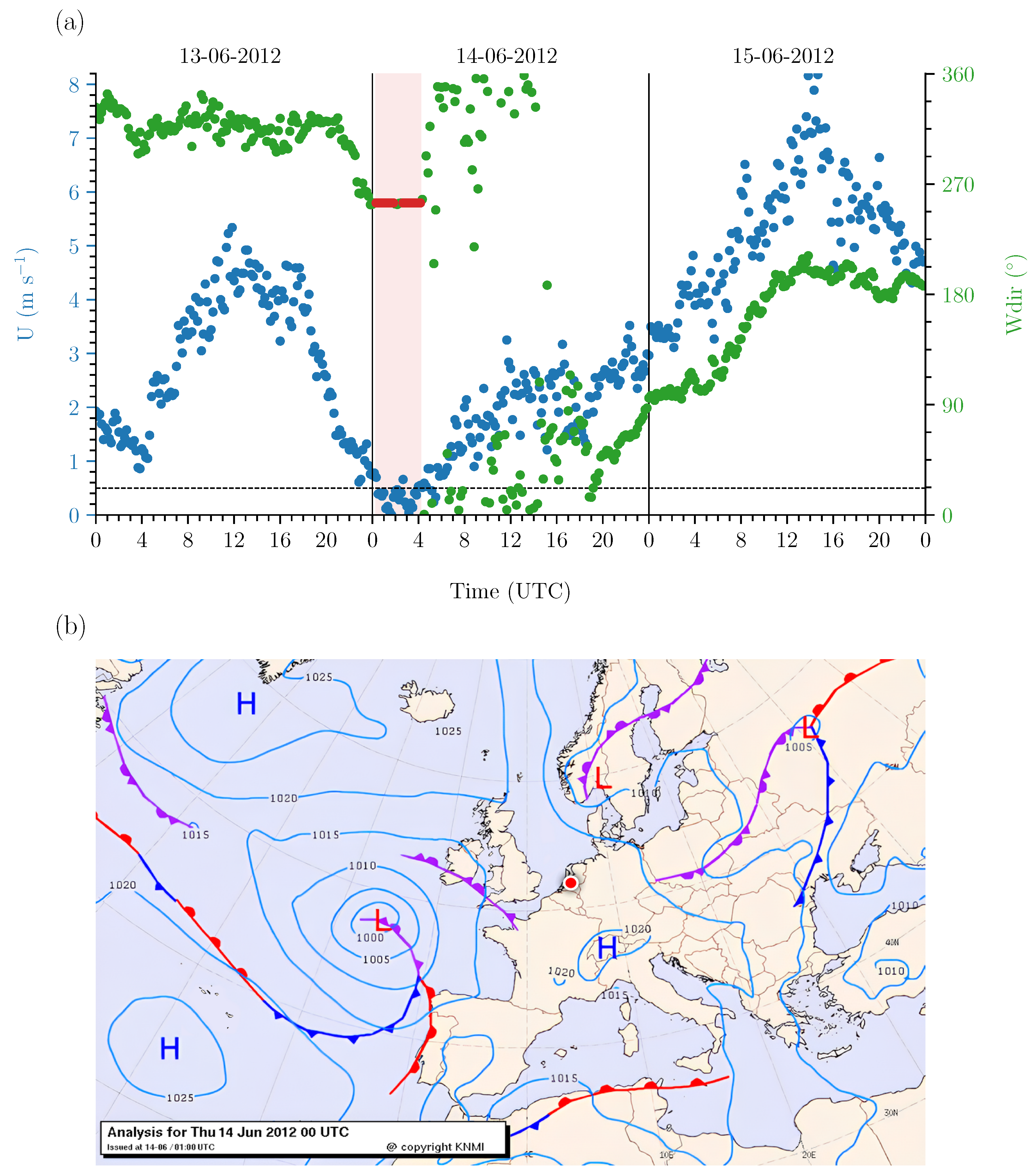
Wind vane stalling is identifiable as a static signal for wind direction, but it can occur due to multiple causes. Moreover, distinguishing mechanical failure from an exceptionally steady flow, or lack thereof, is not always straightforward. An example of a stalling event which appears as a constant wind direction at 10 m which occurred during low wind speed is displayed in Figure 2a. The corresponding meteorological situation can be deduced from the corresponding synoptic map from 14 June 2012 (Figure 2b). The synoptic overview indicates that the Netherlands was influenced by a high-pressure ridge that developed in the days leading up to 14 June. This ridge formed because a low-pressure system near the British Isles intensified while moving in a north-easterly direction. Eventually, a well-developed occlusion front from this low-pressure system passed over the Netherlands later on 15 June. This front was associated with precipitation and an increase in wind. These conditions are reflected in the 10-min averaged wind speed and direction (Figure 2a). The conditions on 13 June are characterised by a clear diurnal variation in the wind speed, with a maximum wind speed of ±6 m s−1 around 14 UTC. The wind direction remained relatively constant, predominantly west to north-westerly, which is consistent with the anti-cyclonic flow in the high-pressure ridge over Central Europe. The wind direction became static 2.5 h after sunset (22:30 UTC) and the wind vane stalled for a prolonged period throughout the night leading into 14 June. We can see that the wind vane stalled as a result of the wind speed, which dropped below 0.5 m s−1. Later stalling instances were observed, broken by a period of slight wind, highlighting the subtlety involved in causing and identifying wind vane stalling. In such cases, not only the accuracy of these readings is questionable but also the meaningfulness of wind direction values, and therefore we aim to identify these events during quality control.
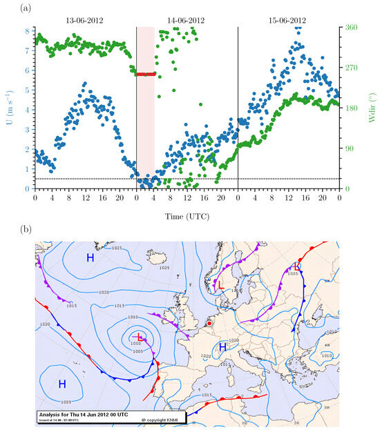
Figure 2.
(a) Ten-minute averaged wind speed (U, blue) and wind direction (, green) in situ measurements at 10 m during a wind vane stalling event (red) on 13–15 June 2012. The dashed horizontal line indicates low wind speeds (<0.5 m s−1). (b) Synpotic situation above Europe during the wind vane stalling event, showcasing the extended high-pressure system over Central Europe and the approaching low-pressure system above the British Isles. The red/white circular marker indicates the location of the Netherlands, where Cabauw is located (refer to Figure 1a).
In this example, we could identify wind vane stalling by employing outlier detection methods: a wind direction that is non-deviating and is also accompanied by a below-limit wind speed. Although such events can be detected, this approach is not without limitations, and the underlying cause remains uncertain. Therefore, wind vane stalling is well-suited for assessing the suitability of data-driven machine-learning methods for data quality control. We utilise its identifiability through outlier detection to train machine-learning methods and evaluate their potential for advancing data quality assurance. In the following sections, we conduct an extended analysis to investigate which (combination of) meteorological variables measured at Cabauw are indicators for wind vane stalling at 10 m. For example, atmospheric stability (Figure 2b), or temperature and moisture, may influence the movement of this wind vane instrument, which has a static friction threshold (determined in wind tunnel: 0.8 m s−1 or 0.4 m s−1 when aligned 10° or 90°, respectively, with respect to the wind). Fortunately, the Cabauw site offers an extensive range of in situ observations which can provide valuable insight into the surrounding meteorological conditions, helping to detect potentially inaccurate wind direction observations. In Section 4.1, we first identify and analyse the wind vane stalling events and conditions statistically, to both apply and corroborate the machine-learning results.
3. Methods
3.1. Meteorological Data and Instrumentation
This study uses 10-min averaged meteorological data from the Cabauw observational site from 2001 to 2022 (22 years), which are validated and publicly available on the KNMI Data Platform(https://dataplatform.knmi.nl/ (accessed on 6 January 2025)). These data have been processed to address known issues (i.e., power outages, mechanical failure, etc.), thereby allowing us to focus on the environmental factors involved during wind vane stalling (e.g., low wind speeds or ice accumulation). Currently, data quality assurance at Cabauw is primarily managed through extensive manual filtering, aided by some automated checks which include validations to ensure data continuity, threshold testing, and cross-checks between sensors to confirm physical feasibility. However, given the complexity and variability of the instrument network, these automated procedures are not uniformly implemented across all sensors. Consequently, all data are extensively reviewed by expert analysts before their release for global use.
The observations used in this study are generated by the following instruments, which are maintained in accordance with WMO standards [15]. Although we focus on the wind direction at 10 m, an extensive array of real-time observations are available to establish the meteorological conditions at the site during wind vane stalling events. Relevant meteorological data are gathered from the multiple masts and sub-sites, as shown in Figure 1. More specifically, we consider the wind direction and speed, temperature, dew point temperature, visibility, and relative humidity, measured at 10, 20, 40, 80, 140, and 200 m. Additionally, temperature, relative humidity, and visibility are also measured at 1.5 m. The wind speed and direction are measured using a KNMI-manufactured cup-anemometer and wind vane combination, as detailed in Section 2. Until 2010, air temperature and specific humidity were measured using KNMI Pt-500 elements and Vaisala HMP243 heated relative humidity sensors. Afterwards, these instruments were upgraded to a Pt-1000 element and EpulsE 33 polymer dew-point temperature sensor. Visibility at each level is measured using the Biral SWS-100. Technical specifications are detailed in Bosveld et al., 2020 [16].
These measurements are used to derive various parameters and metrics which provide additional meaningful insights. From the relative humidity and temperature, the specific humidity and potential temperature are approximated at each height by using a lapse rate for surface pressure (measured at 0.8 m) with −0.125 hPa m−1. Although most variables considered in our analysis are averages of the measurements, we also assess the relevance of the standard deviation and calculate additional potentially indicative parameters based on the findings during our statistical analysis. More specifically, potential temperature, the corresponding lapse rate with height, the dew point depression, and the Fog Stability Index are calculated, as detailed in Section 3.2. The relevant variables considered for machine learning are summarised in Table 1.

Table 1.
Meteorological variables (features) from the Cabauw observational site that are evaluated for feature selection. Excluding pressure (measured at 0.8 m) and wind, which is measured at 10 m and higher, all variables are available at each vertical level: 1.5, 10, 20, 40, 80, 140, and 200 m.
3.2. Identifying Wind Vane Stalling Events and Atmospheric Conditions
A wind vane is considered stalled when it no longer responds to changes in wind direction, or when no directional changes are occurring. The reported wind direction during stalling is questionable, and these events can be attributed to various meteorological influences. We must investigate these factors and the scope of these events manually through outlier detection before we can train and implement machine-learning methods to address this issue (refer to Section 3.3). Therefore, in Section 4.1 we define and identify stalling events by calculating the gradient in the wind direction over time and record instances where the gradient is zero for two or more consecutive data points (≥20 min). While steady winds can lead to a relatively constant wind direction, we expect that most wind vane stalling events are actually caused by zero or very low wind speeds. Therefore, we only select recorded instances with a constant wind direction gradient when wind speed is light-to-moderate (U ≤ 6 m s−1). These conditions reveal the limitations of outlier detection; while this approach is not entirely definitive, it allows us to gain valuable insights into the meteorological conditions linked to wind vane stalling events.
During the recorded wind vane stalling events, we assess the mean and standard deviation of the meteorological conditions throughout the duration of these events. Furthermore, as discussed in Section 2, conditions of zero or low wind speeds are closely correlated with atmospheric stability, and therefore we also assess the lapse rate of potential temperature ():
where is the difference in potential temperature between the different height levels (). The historic observations from Cabauw reveal that atmospheric stability and low wind speed at this site are often linked to the occurrence of fog, in particular, radiation fog [17]. Radiation fog typically occurs under stably stratified conditions with low wind speeds, serving as a visual indicator for stability [18]. Therefore, (radiation) fog formation can be an informative variable for this particular machine-learning application, providing insights into the atmospheric conditions in which wind vane stalling can occur. To this end, we calculate the potential for fog formation as the height-adjusted dimensionless Fog Stability Index (FSI):
where and represent the air temperature and dew point temperature at 1.5 m, respectively, while and are the air temperature and wind speed observed at height z [17,19]. The three terms in the FSI equation (from left to right) represent the influence of humidity, atmospheric stability, and wind speed. In general, when FSI is low (<30) or negative, there is a high probability of fog formation. In addition to the FSI, we also consider the potential for fog formation by incorporating the dew point depression for each height (the difference between the air temperature and dew point temperature, ).
3.3. Machine-Learning Methods
In this work, we model the wind vane stalling events described in the previous sections by applying a selection of supervised and semi-supervised machine-learning methods. For the supervised learning, we conceptualise the stalling events as a binary classification problem, categorising the data into two classes: non-stalling (0) and stalling (1). We compare five different supervised multi-class machine-learning methods: Logistic Regression (LR) [20], K-Nearest Neighbour (KNN) [21], Random Forest (RF) [22], Gaussian Naive Bayes (GNB) [23], and Support Vector Machine (SVM) [24]. However, due to the inherent data imbalance, which will be described below, we additionally consider one semi-supervised one-class machine-learning method, One-Class Support Vector Machine (OCSVM) [25]. While the supervised multi-class methods learn from both classes, the semi-supervised one-class method only learns from the positive class (stalling). For more detail, Chase et al. 2022 provides more information about these machine-learning methods [21].
To effectively classify wind vane stalling with machine-learning methods, we must train the methods with established stalling events and relevant meteorological variables. Information from the determined wind vane stalling events (refer to Section 3.2) is combined with the available meteorological observations at Cabauw in order to select the most relevant and indicative meteorological variables (hereafter referred to as features) that the methods will use to distinguish between the two classes. The careful selection of features is essential for optimising the performance of the machine-learning methods. In addition to feature selection, we also tune the parameters of the machine-learning methods to maximise their performance metrics, such as precision and accuracy. Furthermore, the dataset has an inherent imbalance. Figure 2a shows that wind vane stalling occurs for a small number of data points throughout the day, if at all. Therefore, the relative number of samples classified as wind vane stalling is expected to be substantially lower. Fitting data-driven methods for binary classification to an imbalanced dataset would yield tools that are biased towards the majority class (in our case, non-stalling events). Consequently, we implement strategies that ensure reliable performance for both classes. In the following, the steps for applying the machine-learning methods are elaborated in more detail.
First, we apply a process of feature selection based on the Mutual Information (MI) score [26]. The MI-score, as defined in Equation (3), is calculated using the Python library scikit-learn. The MI-score systematically computes the interdependence of two random variables, X and Y, by using non-negative score-values. In other words, the MI-score indicates the amount of uncertainty in X due to the knowledge of Y, and vice versa. Therefore, a score of zero indicates that there is no statistical dependence between two variables and is not useful for learning. In the context of wind vane stalling, we limit the possible features to the meteorological variables measured along the vertical masts, as summarised in Table 1. We compare these features to the manually identified stalling cases and calculate the MI-score. Ultimately, we assess and select features for the machine-learning methods with an MI-score above the 25th percentile, which represent the most predictive variables that explain the conditions of wind vane stalling.
Next, a selection procedure is used to optimise the fitting of the machine-learning methods to the selected features. The performance of the machine-learning method is dependent on the balance of the data volume and selected parameters. During the selection phase, the machine-learning methods are subject to a heterogeneous training dataset, while the parameter space of each method is systematically explored. By doing so, we ensure that the trained method performs optimally for unseen testing data, based on the values of the method parameters. We use a grid search approach to systematically explore the different parameters [27]. Grid search is a robust approach that systematically trains the different machine-learning methods by testing all possible combinations of the parameters within predefined limits. In this way, it is possible to identify combinations of parameters that prevent overfitting of the methods or a bias towards one of the classes. The grid search configurations for each machine-learning method are presented in Table 2.
Table 2.
Grid search configuration of parameters for the different machine-learning methods, displaying the range of values and settings for the method parameters to be tuned.
During the fitting procedure, we also address the issue of data imbalance to minimise the biases of the supervised fitted machine-learning methods. The dataset for the wind direction at 10 m is balanced as follows: Identified stalling events throughout the entire period (2001–2022) are recorded, and we retain only a number (n) of non-stalling data points surrounding that event. By applying this method, we focus on balancing the dataset using (meteorological) conditions from data points close to the stalling instance. The balancing method is evaluated by incrementally varying the size of the window by adjusting the number of non-stalling data points up to one hour (6 points) before and after each of the events. Each balanced dataset is then partitioned into training and test sets. To investigate if the training or testing data volumes impact the performance of the different methods, the relative size of each set is varied between 10 and 90%.
Lastly, the multi-class machine-learning methods are evaluated using four established statistical metrics: accuracy, precision, recall, and F1-score [28]. For each machine-learning method, the metrics are calculated and subsequently evaluated to determine if and which data-driven method can suitably distinguish between stalling and non-stalling events. Accuracy represents the overall number of both stalling and non-stalling events that are classified correctly, whereas precision indicates how many of the identified stalling instances were correct. Recall expresses how many of the established stalling instances were correctly identified. The metrics of recall and precision are closely related, and therefore the F1-score combines them into a single metric, providing a balanced assessment of the performance of each machine-learning method. In the context of this study, these metrics indicate each method’s ability to effectively distinguish between stalling and non-stalling data points.
In contrast to the multi-class machine-learning methods, the one-class method is trained solely on stalling instances and is therefore subject to different performance metrics. This method is evaluated by assessing the error in classifying inliers (correctly classified as stalling) and outliers (incorrectly classified as stalling).
4. Results and Discussion
We begin by analysing wind vane stalling events at 10 m throughout the entire period, determining the frequency and associated meteorological conditions during and preceding the stalling event. Next, we determine which supplementary observations (features) are the most informative for the machine learning to identify stalling events. The selected features are then used by the supervised and semi-supervised methods to classify stalling events and their performance is evaluated.
4.1. Meteorological Conditions During Wind Vane Stalling
To better understand wind vane stalling at the Cabauw site and establish training and testing datasets, we begin by analysing the stalling at each height along the masts and across various temporal scales. Here, we identified wind vane stalling (detailed in Section 3.2) using outlier detection. Between 2001 and 2022, a total of 1456 wind vane stalling events across all heights were reported (per height: 315, 206, 282, 213, 224, and 216 cases for heights from 10 to 200 m, respectively). The percentage of time that the wind vane at each height stalled throughout the entire 22 years is shown in Figure 3a. In general, we observe that, at each height, the wind vane stalled approximately 3–4% of the time (cumulative ∼11–15 days annually). The relatively high frequency observed at 40 m is likely related to the base of the tower influencing the turbulence at that height. Nonetheless, as expected, stalling occurs most frequently at the 10 m level (4.54%) because the wind speed is lowest near the surface. Due to the higher frequency of events, this height is chosen for the remainder of our analysis because more stalling instances facilitate more effective machine learning from the data.
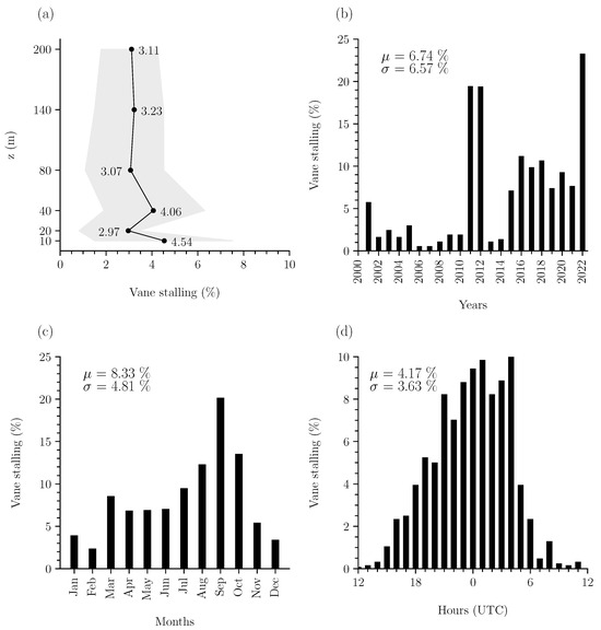
Figure 3.
The frequency of wind vane stalling at Cabauw. (a) Average percentage (markers) and standard deviation (shaded) of time the stalling at each vertical level from 2001 to 2022. Average relative time the wind vane at 10 m stalled each (b) year, (c) month, and (d) hourly. Figures (a,c,d) exclude the outlier years: 2011, 2012, and 2022. Mean () and standard deviation () values of the yearly, monthly, and hourly distributions are displayed within the plots.
Figure 3b shows the relative occurrence of wind vane stalling at 10 m for each year. Distinct yearly variations are observable throughout the entire period. For instance, for more than half of the years, stalling occurred less than 5% of the time; meanwhile, stalling occurred up to 20% of the time during other years. Although stalling appears more frequent after 2014, no clear trend emerges from the yearly distribution. The years 2011, 2012, and 2022, which exhibit significantly more stalling (p-values < 0.05 and z-scores (distance from the mean in standard deviations) ≥ 2), were reported as ‘extremely sunny’ [29,30]. In fact, 2022 set the record as the sunniest year in the Netherlands since measurements began in 1901 [31]. The prevalence of sunny conditions suggests that these years experienced a higher frequency of fair weather, which is often associated with lower wind speeds. Fair weather typically results from high-pressure systems, in which cooler air subsides, inhibiting convection at the surface. As a result, stable atmospheric conditions develop, limiting or preventing horizontal air movement and leading to low wind speeds. Climate change may exacerbate such extreme conditions, causing more frequent low wind scenarios, which is highly relevant to various industries. However, we exclude these outlier years (2011, 2012, and 2022) from further analysis in order to focus on assessing more typical stalling behaviour.
A more discernible pattern emerges when examining seasonal variations. Figure 3c shows the average relative wind vane stalling occurrence at 10 m for each month. Two distinct periods with increased wind vane stalling emerge: spring months to early summer (March–July), and even more during the late summer to early autumn (August–October). We observe that wind vane stalling is more likely during these periods, peaking significantly during September (p-values < 0.05 and z-scores ≫ 2) where stalling occurs ± 20% of the month on average (cumulative ∼6 days). The increased frequency of stalling during these months may be attributed to the large-scale dynamics. For the Netherlands, both March–May and August–October are seasons with a higher tendency for fair weather conditions as high-pressure areas dominate across Southern-to-Central Europe [32], favouring fair weather, and thus lower wind speeds to occur.
Diurnal variations in air flow are also expected to influence wind vane stalling. To this end, Figure 3d shows the frequency of wind vane stalling at 10 m on average for each hour. We observe a parabolic-shaped diurnal pattern, such that wind vane stalling occurs most frequently (approximately 90% of the time) during nocturnal conditions (18–6 UTC). The example case from Figure 2 supports the suggested relationship between low wind speeds, (nocturnal) atmospheric stability, and wind vane stalling at the 10 m level. To further investigate this relationship, we also consider additional in situ observations that can offer insight into the meteorological conditions surrounding the events.
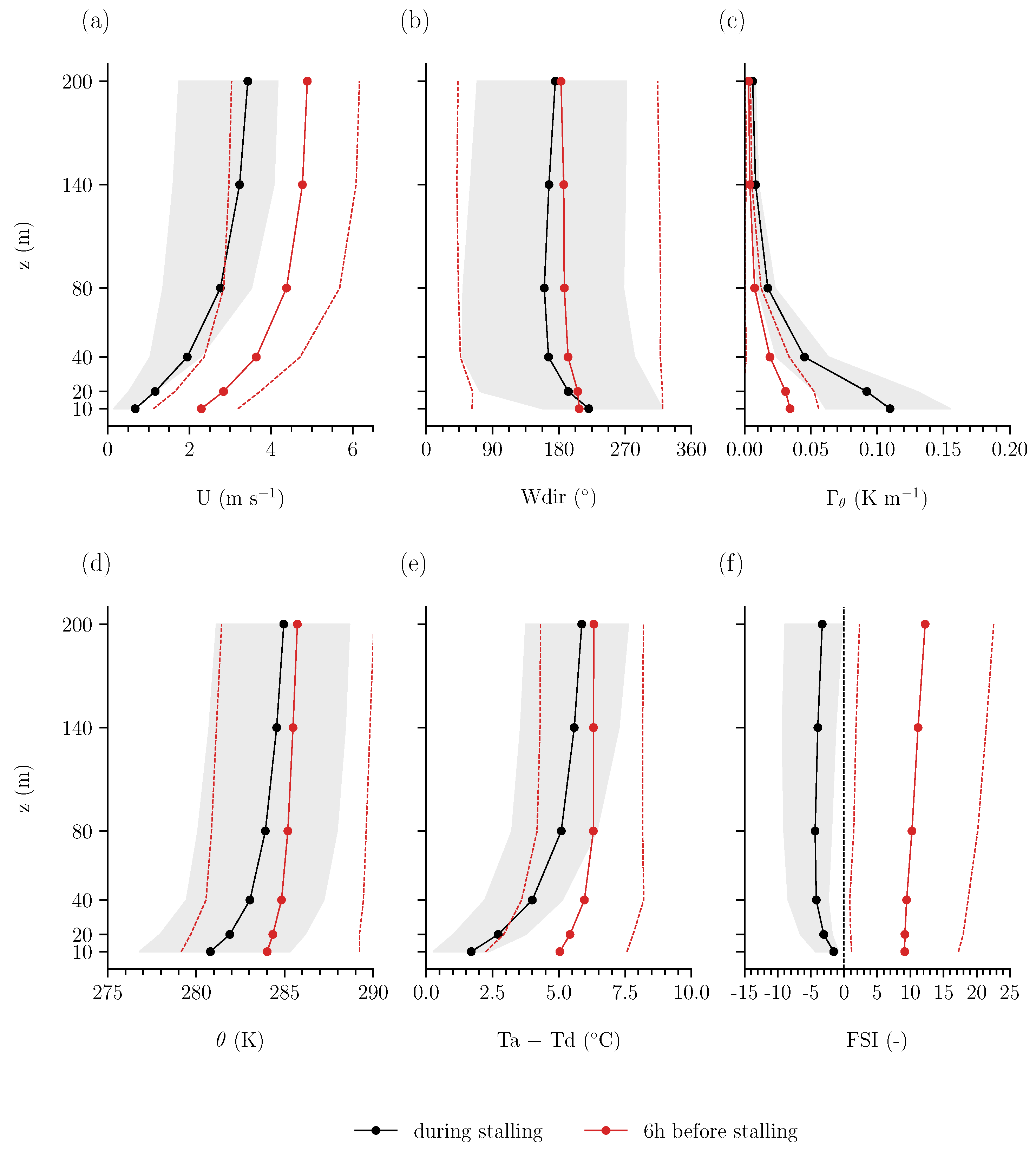
The meteorological conditions preceding and during stalling events offer additional insight into the underlying causes. Figure 4 displays the average vertical profiles of the measured wind speed (U), wind direction (), potential temperature (), lapse rate (), dew point depression (), and Fog Stability Index (FSI). The black line indicates the average vertical profile when the stalling event occurs at 10 m, and the red line represents the average profile six hours prior to the stalling event. The average wind speed profile (Figure 4a) during wind vane stalling at 10 m displays the characteristic logarithmic shape with height, where the lowest values are observed at the 10 m level, as anticipated. Notably, the average wind speed at each height leading up to the stalling event at 10 m is also low (U m s−1), and decreases further during the event, diminishing by roughly 2 m s−1 within the lowest 20 m. Most importantly, at 10 m, the wind speed is typically less than 1 m s−1 during the stalling event, suggesting that the primary cause of wind vane stalling can be attributed to low wind speed and that freezing/ice accumulation or other environmental factors are likely negligible. Furthermore, in Figure 4b, we observe a high standard deviation in wind direction, suggesting that no distinct wind direction is prominent, prior to or during stalling events. This result emphasises that the reported wind direction values are less meaningful during these events.
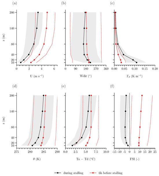
Figure 4.
Average vertical profile of meteorological variables at each height during (black) and six hours before (red) wind vane stalling events at 10 m throughout 2001–2022 (excluding 2011, 2012, 2022): (a) wind speed (U), (b) wind direction (), (c) lapse rate of potential temperature (), (d) potential temperature (), (e) dew point depression (), and (f) Fog Stability Index (FSI). The grey shaded areas and red dotted lines indicate the standard deviation during and preceding the stalling event, respectively.
As alluded in Section 2, the prevalence of low wind speed depends on the atmospheric boundary layer conditions. Regarding the atmospheric stability, and (Figure 4c,d) exhibit relatively cooler average temperatures and strong gradients near the surface when stalling occurs at 10 m. The average potential temperature at 10 m is too high for freezing to occur, further supporting that most stalling events are not caused by this mechanical restriction. Furthermore, we determined that the majority of the wind vane stalling instances at 10 m (94.43%) are associated with an average air temperature, > 0°C.
Below 80 m, we observe stable conditions where the lapse rate is 0.10 K m−1. Moreover, relatively colder air (roughly 5 °C) is able to reside within this layer, pushing the warmer air aloft, creating stable (stratified) conditions. Additionally, we determined that the mean surface pressure during wind vane stalling is 1022 hPa. These findings corroborate that stable stratification of the lower atmosphere is a common condition for wind vane stalling at 10 m. By assessing the profiles six hours prior to the stalling event, we observe a clear development of this stability as the lapse rate increases by 0.05 K m−1.
These developing stable conditions allow for radiation fog formation, which can therefore serve as an indicator for wind vane stalling. This type of fog occurs in colder or nocturnal conditions with (strong) radiative cooling, provided that there is sufficient moisture available [18]. The potential of fog formation is highlighted by the dew point depression and FSI (Figure 4e,f). We observe that the average difference between air temperature () and dew point temperature () during wind vane stalling is 2.5 °C in the lowest 20 m (where is generally between 0 and 10 °C). Therefore, air saturation is probable, as is resultant fog formation in the lower atmosphere. The FSI metric further supports the likelihood for fog formation as it decreases leading up to the wind vane stalling event, with negative or near-zero values indicating a very strong probability of fog formation. The probability for fog formation is corroborated by the fact that the visibility measured at 1.5 m is almost four times lower during wind vane stalling than six hours prior, decreasing from 25 km to only 6 km.
In the context of wind vane stalling, the observed relationship between low wind speeds, atmospheric stability, and fog formation is also consistent with previous research. In 2018, Izett et al. conducted a study of 254 fog events at the Cabauw site between 2012 and 2016 [17], categorising them using the methodology outlined in Menut et al., 2014 [33]. The authors classified the majority of fog events as radiation fog (63.4%), occurring under stable, stratified conditions in the lower atmosphere. Moreover, these fog events primarily occurred between 18 and 8 UTC, during the months of January, February, and March, as well as August, September, and October. Although wind vane stalling was less frequent during winter months, this pattern reflects the relatively high frequency of wind vane stalling that we observed in March, August, September, and October, also occurring between 18 and 8 UTC. Therefore, fog formation may also serve as an indicative variable for machine-learning methods towards identifying wind vane stalling events.
4.2. Feature Evaluation
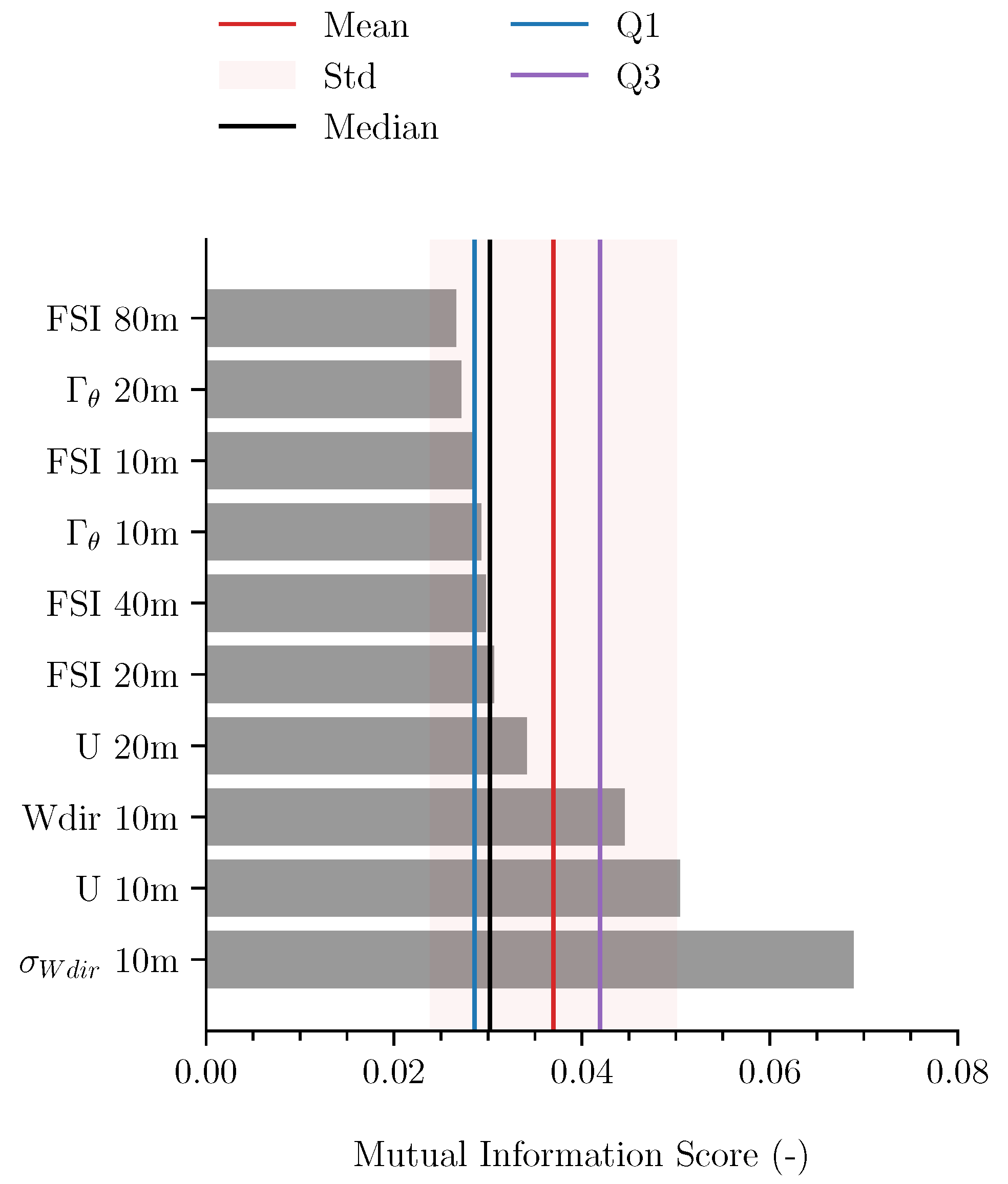
We use an MI-score (see Section 3.3) to evaluate which features (variables) are most effective in training the machine-learning methods to predict wind vane stalling at 10 m. We evaluated 12 different meteorological variables measured at heights ranging from 1.5 to 200 m (see Table 1). Of the 60 evaluated features, Figure 5 shows the ten highest-ranked features based on their MI-score alongside the mean, median, standard deviation, and inter-quartile range of the MI-score of all evaluated features. As expected, the variation in wind direction (standard deviation: ) and wind speed (U) at 10 m are the most relevant determining features regarding the behaviour of the wind vane sensor at 10 m. However, the wind direction and speed at higher levels was not as indicative. In fact, we observe that the remaining most influential features are predominantly related to stability.

Figure 5.
Ten highest-ranked features based on calculated Mutual Information (MI) score. The features evaluated are those listed in Table 1. The MI-scores are presented alongside the mean, median, standard deviation, and inter-quartile range (Q3–Q1) of the MI-score of all evaluated features.
This established relevance of the stability parameters is consistent with the findings of the previous section, given that wind vane stalling was observed predominantly during (nocturnal) stable atmospheric conditions in the lower 20 m of the atmosphere. Furthermore, the MI-score suggests that, in addition to the 10 m level, stability features at the 20, 40, and 80 m levels are also related and can explain part of the variability in wind vane stalling at the 10 m level. Moreover, the relatively high MI-score of these features at different heights emphasises that the influence of stability is not limited to what is observable at the 10 m height of the wind vane and larger-scale processes are at play. These results corroborate observations from our statistical analysis in Section 4.1. However, beyond the case study of wind vane stalling, our findings demonstrate that machine-learning methods can be applied to atmospheric phenomenon to identify relevant parameters which can then be cross-referenced for data quality assurance. Additionally, this knowledge can enhance outlier detection such that events identified outside of these conditions can be flagged as suspicious.
Though these ten variables are the highest-ranked, the MI-score itself also provides insight into the meteorological conditions surrounding wind vane stalling events. For instance, specific humidity, air pressure, and air temperature reported low to near-zero MI-scores, especially at the highest levels of 140 and 200 m. Also, visibility (meteorological optical range), which depends on fog formation, ranked 15th. These values suggest that wind vane stalling at 10 m is relatively independent of the temperature and humidity higher in the boundary layer. Additionally, when evaluating which features emerge as the most relevant for particular meteorological seasons (spring, summer, autumn, and winter), no significant differences were observed. As these ten features consistently emerge as dominant across all seasons, no significant differences in behaviour of the machine-learning methods are anticipated under varying seasonal meteorological conditions. However, different variables are expected to be indicative for other meteorological phenomenon, or even wind vane stalling at other heights, and these methods can provide useful insight.
Our findings confirm that anticipating wind vane stalling events goes beyond simply assessing the current status of the wind at 10 m. The variables with a high MI-score enhance our understanding of the meteorological conditions surrounding these events and can be applied with multi-class and one-class machine-learning methods. To this end, we select the features with an MI-score above the 25th percentile (Q1): and at 10 m, U at 10 and 20 m, FSI at 20 and 40 m, and potential temperature lapse rate () at 10 m.
4.3. Supervised Multi-Class Evaluation
We first assess the performance of five supervised multi-class machine-learning methods using the seven relevant features selected in the previous section. As outlined in Section 3.3, each method is trained to classify stalling and non-stalling events using these features. During the training phase, the available data are incrementally balanced by retaining n-points of non-stalling data up to one hour (6 points), both before and after each stalling event, to obtain a balanced dataset with which we can evaluate the performance of the machine-learning methods. Furthermore, the division of the data into training and test datasets is varied. During training, the optimal configuration is determined through grid search, using the (incrementally balanced) data for each partitioning of the training and test datasets.
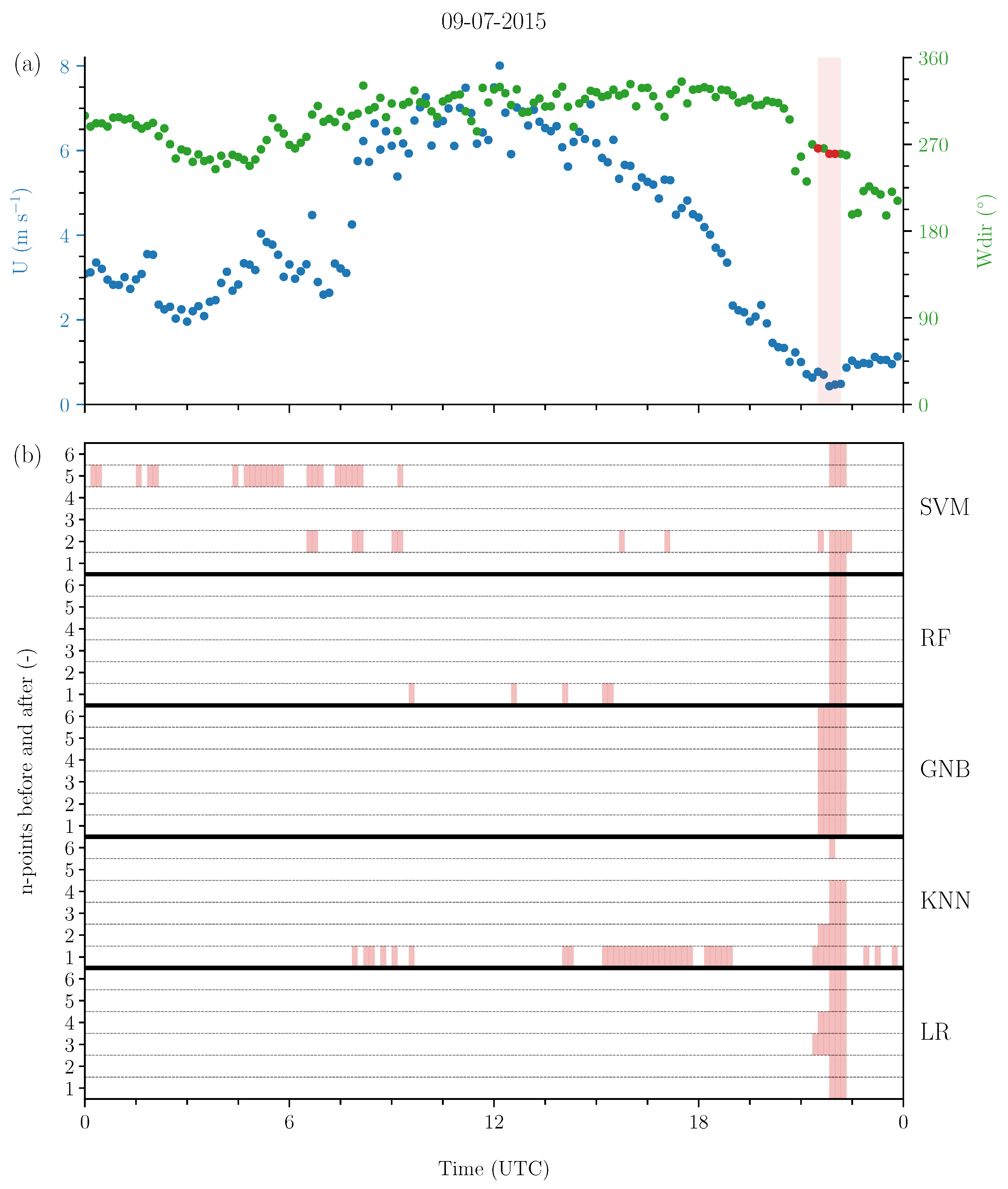
To illustrate the performance of the machine-learning methods during a wind vane stalling event, Figure 6 displays a time series of wind speed and direction alongside the output from the machine-learning methods on 9 July, 2015. The figure also showcases our approach to incrementally balance the dataset where different time windows influence the results. This example utilises a typical 80/20 division of training and test data (80% training data, 20% test data) across all machine-learning methods with the best configured parameter combinations. Figure 6 demonstrates that most of the machine-learning methods explored in this study are capable of successfully identifying a stalling event, with varying performance depending on how the dataset is balanced. More specifically, in this example, we observe that each of the five selected machine-learning methods correctly identify the wind stalling event, and GNB, RF, and LR exhibit the least classification errors. Including data points close to the wind vane stalling event can enhance the performance of most methods. However, KNN and SVM demonstrate greater difficulty in accurately identifying the stalling instance, either reporting its occurrence too often or failing to detect it altogether. It is important to note that the performance observed during this specific wind vane stalling event is not necessarily representative of all events. Therefore, we analyse the overall performance over 22 years using a set of metrics, which are used to evaluate the performance of the machine-learning methods with the best configured parameter combinations (summarised in Figure 7).
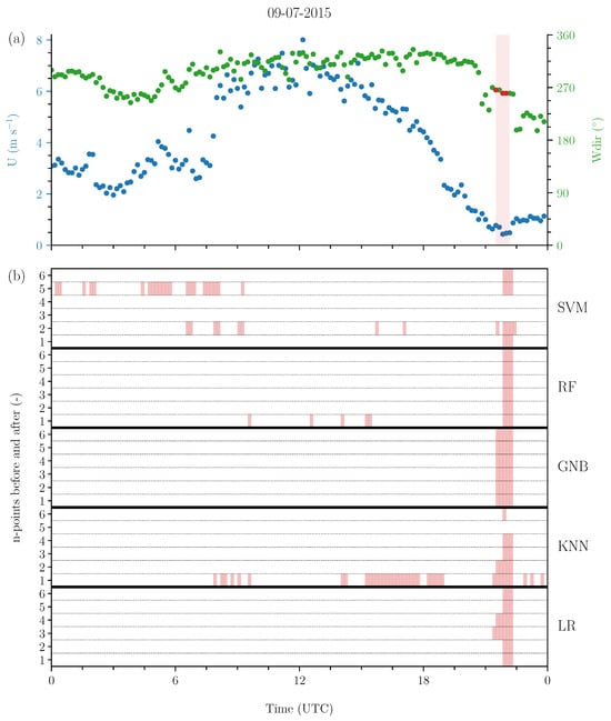
Figure 6.
(a) Ten-minute averaged wind speed (U) and wind direction () at 10 m on 9 July 2015, showcasing a wind vane stalling event (red). (b) Identified instances of wind vane stalling by five supervised multi-class machine-learning methods shown for incrementally balanced data by n-points before and after the wind vane stalling event. The five methods are Logistic Regression (LR), K-Nearest Neighbour (KNN), Gaussian Naive Bayes (GNB), Random Forest (RF), and Support Vector Machine (SVM).
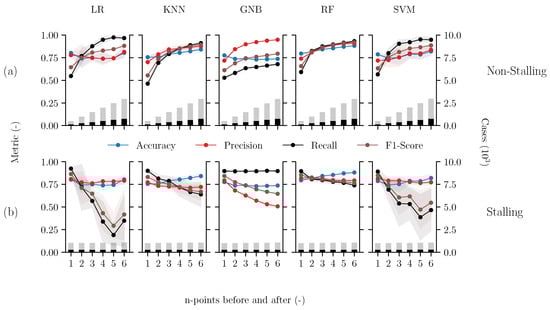
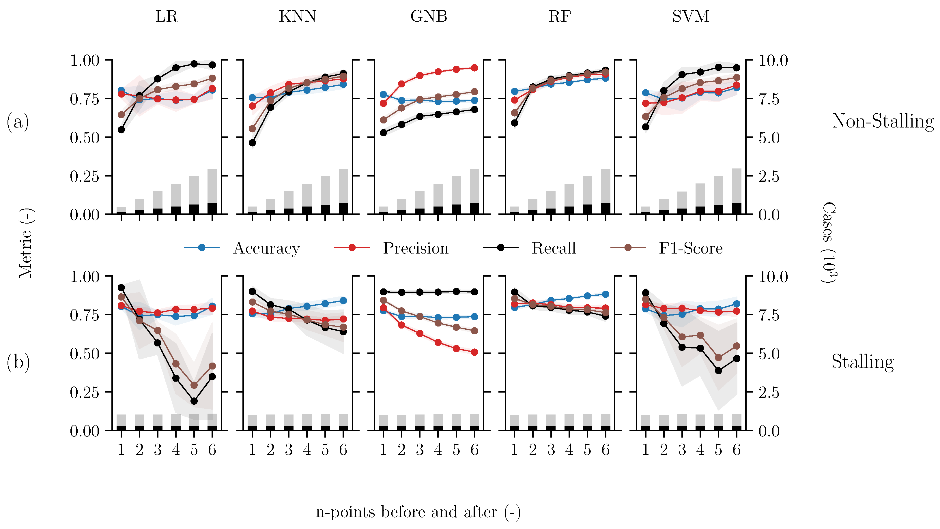
Figure 7.
Performance metrics (Accuracy, Precision, Recall, and F1-score) of supervised multi-class machine-learning methods which are incrementally balanced by n-points before and after the wind vane stalling event at 10 m. The five methods include Logistic Regression (LR), K-Nearest Neighbour (KNN), Gaussian Naive Bayes (GNB), Random Forest (RF), and Support Vector Machine (SVM), which are evaluated based on their ability to classify (a) non-stalling and (b) stalling events. Additionally, the number of classified test cases (bars) is displayed on the right y-axis (×103). The solid markers represents the average result while varying the training and test dataset sizes. The partitioning varies between 10 and 90%, and the range of the results is represented by the shaded area.
Figure 7a,b show the performance metrics (Accuracy, Precision, Recall, and F1-score) for each of the five multi-class machine-learning methods, regarding their ability to classify points as non-stalling and stalling, respectively. These metrics describe the ability of the machine-learning methods to correctly identify whether a data point represents a wind vane stalling event or a non-stalling event. As mentioned, the performance of the machine-learning methods depends on how the training dataset is balanced (bars). With this balancing approach, as the number of data points retained before and after a stalling event increase (n), the number of stalling cases remains constant while reported cases of non-stalling linearly increase. The shaded area (grey) represents the range of the values based on how the dataset was divided into training and test sets.
Overall, we observe that both the non-stalling and stalling performance metrics are significantly affected by incrementally balancing the dataset. In particular, for each of the machine-learning methods, the non-stalling performance metrics (Figure 7a) significantly improve, approaching a value of 1, when more non-stalling points are included for training. In contrast, as more non-stalling events are retained, the performance metrics for identifying stalling events (Figure 7b) worsen in most cases, some even approaching <0.5. This behaviour is expected when the dataset becomes more biased towards non-stalling events. Due to this clear impact on each method’s performance, we first consider a suitable balance before analysing these metrics in more detail.
Effective supervised multi-class methods require data balance, and therefore it is recommended to achieve a balance between stalling and non-stalling events. Training with a balanced dataset ensures that the machine-learning methods perform optimally in distinguishing between both of these classes. In this case, achieving this balance depends on optimally defining the time window before and after the stalling event, such that the methods can learn the distinction. Comparing the performance of the different methods in Figure 7, we observe that the performance metrics for classifying both non-stalling and stalling events are balanced when retaining roughly two to three data points before and after the event (40 to 60 min window). We observe that when n = 2–3, nearly all performance metrics for the five machine-learning methods exhibit a sharp increase or decrease for identifying non-stalling and stalling events, respectively. Therefore, with this data balance, many of the supervised multi-class methods demonstrate good performance in effectively distinguishing the data.
Although we observed that each supervised multi-class method generally benefited from a similar data balance, these different machine-learning methods yield varying performance results. Overall, we observe that the GNB method demonstrates the lowest performance, exhibiting a clear bias toward the majority class (non-stalling data points). The accuracy of identifying non-stalling cases increases, approaching 1, if trained with an imbalance. However, the accuracy of identifying stalling cases plummets from approximately 80% to 50%. The precision and F1-score show similar trends. In contrast to GNB, the KNN and RF methods demonstrate relatively stable performance as the dataset becomes more saturated with non-stalling data points. Even with the largest window (n = 6, total 120 min), most performance metrics are >0.75 for classifying both stalling and non-stalling cases. When the datasets are balanced (n = 2), KNN and RF identify stalling events with an accuracy of 0.76 and 0.82, respectively, demonstrating that both methods show potential for identifying wind vane stalling events. Furthermore, the F1-score of KNN and RF are 0.77 and 0.82, respectively. The relatively higher F1-score for RF indicates that this method is better at correctly identifying wind vane stalling events, while making fewer mistakes by missing or incorrectly identifying them. The LR and SVM methods perform similarly to KNN and RF for classifying non-stalling events; however, the F1-score indicates drastically poorer performance for classifying stalling events. Furthermore, both methods also exhibit a high sensitivity to the volume of data used for training and testing, as indicated by the shaded grey area.
Our results establish that while KNN and RF yield promising performance metrics, data imbalance poses a significant challenge affecting all five supervised multi-class machine-learning methods. While we demonstrate which supervised machine-learning methods have the most potential, this methodology may be insufficient for comprehensively addressing wind vane stalling because these events can be subtle and may manifest outside the predefined boundaries. Moreover, directly implementing these methods in a practical, real-time application along the Cabauw tower requires further development. We anticipate that extending these findings to wind vane stalling at other heights or meteorological phenomenon will depend on different meteorological factors which should be investigated with the MI-score and may yield different performance. Nonetheless, the development of a dedicated filtering system, where the KNN and RF methods function together, can improve the reliability and efficiency needed to meet our data quality standards.
We demonstrate that these machine-learning methods, when appropriately balanced, can significantly enhance the data quality assurance. By flagging suspicious events or corroborating outlier detection, these methods demonstrate considerable potential in addressing wind vane stalling and other similar atmospheric phenomena, ultimately enhancing data quality assurance. Still, we anticipate that the quality control for various meteorological data issues will also be constrained by data imbalance. Consequently, as an alternative approach to this obstacle, we analyse the performance of the one-class machine-learning method in the next section.
4.4. Semi-Supervised One-Class Evaluation
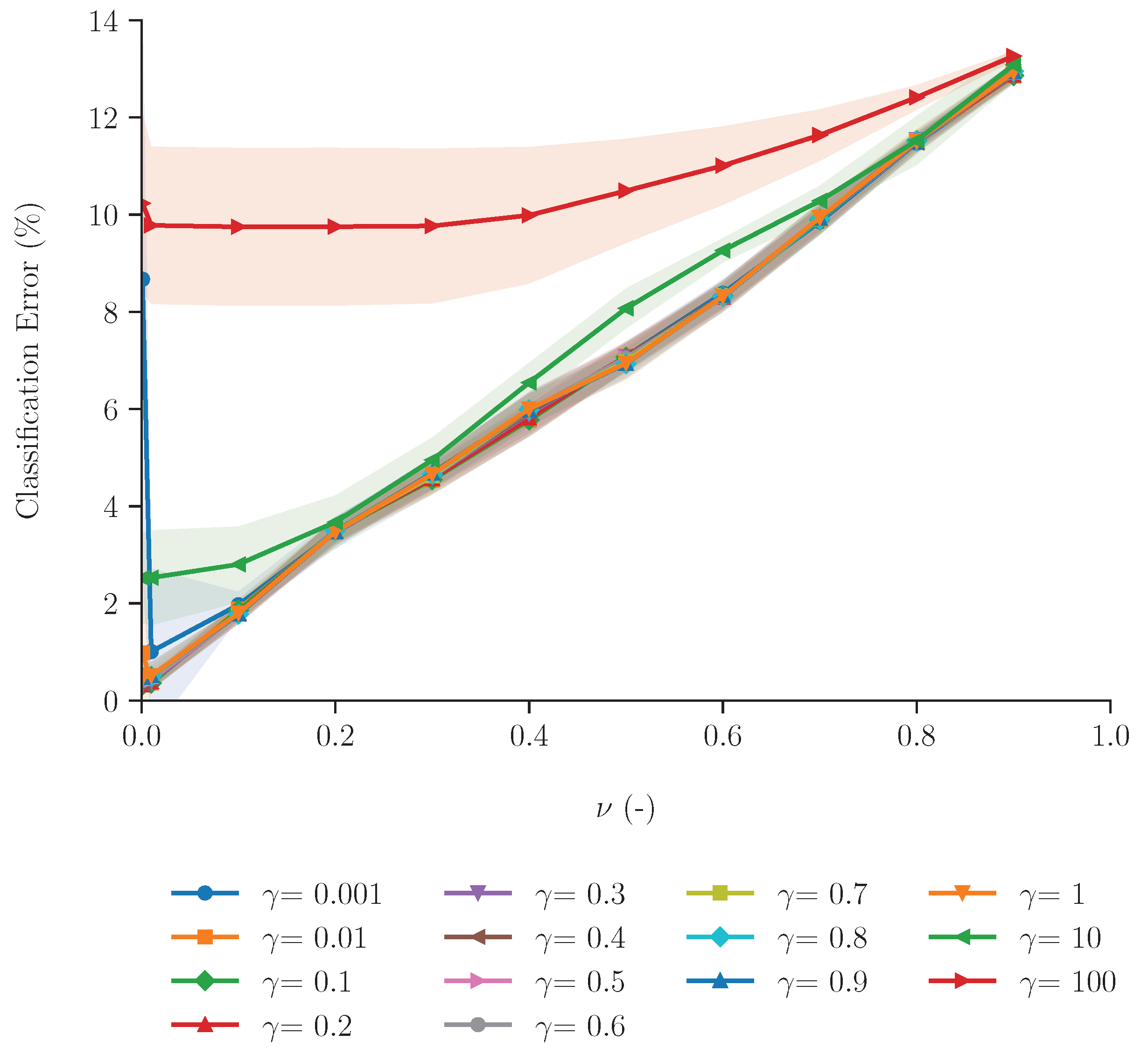
In contrast to the supervised learning methods explored in the previous section, data imbalance does not impact the semi-supervised One-Class Support Vector Machine (OCSVM) method. Moreover, this method learns exclusively from instances classified as stalling, which are considered inliers. The OCSVM method only has two parameters: and (refer to Table 2). The parameter determines the influence of outliers (non-stalling data points), whereas describes the relative influence (dependence) of each data point [21,25]. Due to the single class, we evaluate the performance of OCSVM considering the relative mean error (normalised by the number of cases) for classifying stalling data points. We explore this method’s aptitude by varying the (,)-parameter combinations, as shown in Figure 8.
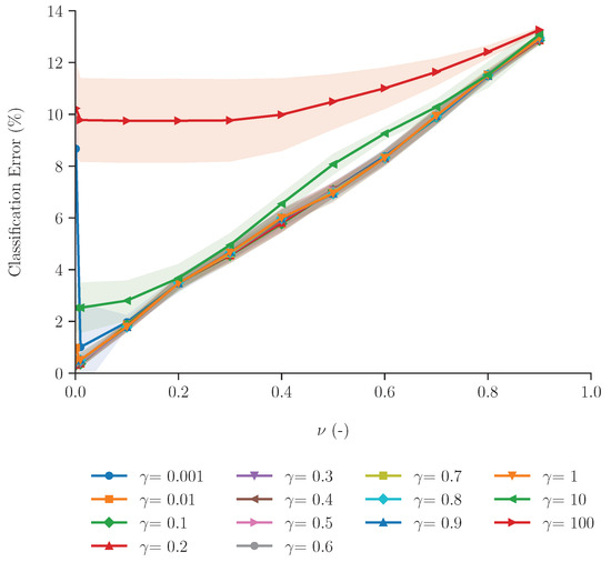
Figure 8.
Evaluation of the One-Class SVM (OCSVM) classifier, showing the relative classification error for the stalling data points depending on varied (,)-parameter combinations. The shaded area represents the range resulting from different training sizes between 10 and 90%, while the solid line represents the mean error.
Figure 8 shows that the number of points that are incorrectly classified as stalling is clearly impacted by the model parameters. We observe that as increases the mean relative error increases. This trend can be attributed to the fact that larger values of allow a larger influence of non-stalling data points, and therefore the method predicts outliers better than inliers. Consequently, for this dataset, should be kept low (<0.5). The influence of is also dependent on . In general, we observe that -values ≤ 1 yield a smaller mean classification error, but the relative influence of becomes higher. As approaches 1, each value yields a relative classification error . Increasing the value of increases the relative dependency of the individual data points. In other words, more data points contribute to the overall performance of the model. Therefore, when combined with a higher , the error is largest, ultimately leading to an overall decrease in this machine-learning method’s performance.
These results suggest that the semi-supervised one-class machine-learning method, tuned with < 0.2 and ≤ 1, could effectively identify stalling data points, with up to 90% accuracy. Furthermore, our findings highlight the importance of the model parameters: the effectiveness of a machine-learning method is not only based on the key features. Considering the classification accuracy, this semi-supervised method shows no significant improvement in performance compared to the two best-performing supervised multi-class methods (KNN and RF). Both supervised and semi-supervised methods can effectively identify the stalling data points. However, unlike supervised methods, this approach circumvents the issue of data imbalance, enabling the development of a more straightforward and practical application. Nonetheless, the one-class semi-supervised method is not without limitations. Due to the fact that this machine-learning method is exclusively designed and validated using the majority class (stalling), developing an effective and practical application still requires further exploration.
Ultimately, both supervised and semi-supervised methods can be developed and integrated at various stages of the data filtering process, improving quality assurance, helping to resolve wind vane stalling events and other meteorological data issues. Our results demonstrate that these methods can provide valuable insight for initial checks, generating warnings based on a range of incoming observations, facilitating manual filtering and improving overall confidence in the data quality.
5. Conclusions
This paper provides insight into the application of machine-learning methods for advancing the quality control of meteorological datasets. To explore this potential, we investigated the application of various machine-learning methods to identify wind vane stalling events at 10 m height. First, we manually identified wind vane stalling instances from 2001 to 2022 (22 years) and shed light on the underlying meteorological conditions during these events to serve as a foundation for machine-learning input and application. In that context, the most indicative variables were selected based on their MI-score and ultimately applied in supervised and semi-supervised machine-learning methods. We evaluated the performance of various methodologies and conditions to provide an indication of which may be most applicable to advancing the data quality assurance of long-term meteorological datasets. The results from this study highlight the potential of using data-driven machine-learning methods towards resolving meteorological data issues and providing high-quality datasets. Not only can machine-learning-assisted quality control increase automatisation potential but can also provide valuable insight into the physical understanding of the data issues.
Our data analysis revealed that wind vane stalling events at the Cabauw site were most commonly associated with low wind speeds in stable atmospheric conditions. Our results showed that wind vane stalling occurred not only at the surface but also at all heights up to 200 m. More specifically, throughout the entire analysis period, stalling occurs roughly 3–4% of the time, where the highest frequency is at the 10 m level (4.54%), as expected. Therefore, this study focused on wind vane stalling at 10 m due the higher number of events, which provides a more robust dataset for machine-learning applications. Furthermore, annual distributions of wind vane stalling frequency at 10 m revealed a consistent increase in stalling in the last decade compared to the first decade, which may have strong implications for wind-related industries. Monthly and hourly distributions showed that wind vane stalling is most frequent during August, September, and October, and predominantly during the nighttime (18 to 6 UTC). These trends suggest that wind vane stalling is characteristic of (but not limited to) stably stratified nocturnal boundary layers, which was also supported by the observed prevalence of radiation fog and strong stability indicated by the lapse rate and vertical potential temperature differences. Additionally, the temperature was too high on average during these event to indicate freezing as a likely cause.
Considering the above findings, an MI-score was calculated for the selected variables to determine how indicative these features were for stalling events at 10 m, using machine learning. Applying these MI-scores, our findings suggested that it is feasible to address this binary classification problem (stalling or not stalling) with a minimal set of the seven most explanatory variables (features) in varying meteorological conditions: , U at 10 and 20 m, and at 10 m, FSI at 20 and 40 m, and at 10 m. Our results show that the highest-ranked features align with the conclusions made through direct identification of stalling events and analysis of the meteorological conditions, particularly regarding atmospheric stability and fog formation. Therefore, in addition to providing further insight and confirmation of our analysis, we demonstrate that such machine-learning methods can be applied to other meteorological phenomenon, determining relevant variables that should be considered when performing quality assurance.
These key features were used as input to train and compare five supervised multi-class machine-learning methods (LR, KNN, RF, GNB, and SVM), while systematically investigating the impact of the inherent data imbalance. Additionally, we evaluated the performance of one semi-supervised one-class method (OCSVM) due to its insensitivity to data imbalance. Overall, we observed that the KNN and RF supervised methods show the highest potential for identifying stalling and non-stalling events, while the GNB method yielded the worst performance metrics. The RF method slightly outperforms KNN, identifying approximately of stalling events when the data are balanced (40 min of non-stalling data retained surrounding the stalling event). Both methods exhibited relatively stable accuracy, precision, recall, and F1-score compared to the other methods, which were strongly influenced by the proportion of non-stalling points retained in the dataset. Due to the relative data scarcity, and therefore imbalance inherent to wind vane stalling events, we do not recommend further investigation into the LR, GNB, and SVM methods. Comparatively, the semi-supervised OCSVM showed promising results in classifying stalling instances due to its reliance on only the positive class (stalling). Although the classification performance was similar to the supervised KNN and RF methods, the fact that OCSVM is not affected by data imbalance is a clear benefit for meteorological data quality issues. Ultimately, we recommend the supervised (KNN and RF) and semi-supervised (OCSVM) methods to investigate meteorological data issues. Although the results in this study demonstrate the potential of applying machine learning to meteorological data quality assurance, adaptations are required for practical implementation. Nonetheless, these methods can be employed to perform initial checks and generate warnings based on diverse incoming observations, thus facilitating manual filtering and strengthening confidence in data quality assurance.
We believe that the benefit of using machine-learning methods for quality assurance is two-fold. First, machine learning has the potential to assess and assure the data quality of the datasets. Machine-learning methods allow data to be automatically and importantly, uniformly treated. Second, the use of machine-learning methods will support research and deepen our understanding of the meteorological conditions and physics influencing data issues. Our results demonstrate how machine learning can be applied, not only to predict but also to diagnose meteorological conditions, enhancing data quality assurance of observational datasets. Furthermore, in contrast to manual or automated outlier detection methods, machine-learning approaches are scalable, ensuring they can be easily maintained and adapted over time. Therefore, based on our findings, which indicate the suitability of various machine-learning methods, we recommend further exploration and eventual implementation of these methods to advance and facilitate data quality control for the Cabauw observational site and other meteorological observation sites across the Netherlands which use similar equipment.
Author Contributions
Conceptualisation, results and visualisation, V.S.d.F.; writing, V.S.d.F., J.M.I.S. and I.G.-M.; supervision, J.M.I.S. and I.G.-M. All authors have read and agreed to the published version of the manuscript.
Funding
This research received no external funding.
Data Availability Statement
The development of this work has been carried out using well-known Python libraries for modelling (e.g., scikit-learn) and visualisation (e.g., matplotlib). A complete Python implementation of the applied methods is available in the corresponding 4-TU repository which can be accessed through https://doi.org/10.4121/6bee84b7-0088-4232-badb-9b3b38a3c40e, accessed on 6 January 2025.
Acknowledgments
The foundational work for this publication was carried out in 2023 during an MSc internship by the first author, hosted by the KNMI as part of the MSc Earth & Environment programme at Wageningen University & Research. Special thanks are extended to the members of the Cabauw In-situ team for their warm welcome and insightful scientific contributions which helped shape this research.
Conflicts of Interest
The authors declare no conflicts of interest.
Abbreviations
The following abbreviations are used in this manuscript: Royal Netherlands Meteorological Institute (KNMI); Baseline Surface Radiation (BSRN); Profiling Site (PS); Automatic Weather Station (AWS); Energy Balance terrain (EB); World Meteorological Organisation (WMO); wind direction (Wdir); wind speed (U); difference in potential temperature (dθ); difference between height levels (dz); Fog Stability Index (FSI); air temperature (Ta); dew point temperature (Td); Logistic Regression (LR); K-Nearest Neighbours (KNN); Random Forest (RF); Gaussian Naive Bayes (GNB); Support Vector Machines (SVM); One-Class Support Vector Machines (OCSVM); relative humidity (RH); specific humidity (q); air pressure (p); visibility (ZMA); potential temperature (θ); potential temperature lapse rate (Γθ); standard deviation wind direction (σwdir); Mutual Information (MI).
References
- Alley, R.B.; Emanuel, K.A.; Zhang, F. Weather: Advances in weather prediction. Science 2019, 363, 342–344. [Google Scholar] [CrossRef]
- Bauer, P.; Thorpe, A.; Brunet, G. The quiet revolution of numerical weather prediction. Nature 2015, 525, 47–55. [Google Scholar] [CrossRef] [PubMed]
- Lam, R.; Sanchez-Gonzalez, A.; Willson, M.; Wirnsberger, P.; Fortunato, M.; Alet, F.; Ravuri, S.; Ewalds, T.; Eaton-Rosen, Z.; Hu, W.; et al. Learning skillful medium-range global weather forecasting. Science 2023, 382, 1416–1422. [Google Scholar] [CrossRef] [PubMed]
- Beljaars, A.C.M.; Bosveld, F.C. Cabauw Data for the Validation of Land Surface Parameterization Schemes. J. Clim. 1997, 10, 1172–1193. [Google Scholar] [CrossRef]
- van der Vliet, J. Elf Jaar Cabauw-Metingen; Technical Report; Royal Netherlands Meteorogical Institute: De Bilt, The Netherlands, 1988. [Google Scholar]
- Bosveld, F.C.; Baas, P.; Beljaars, A.C.; Holtslag, A.A.; de Arellano, J.V.G.; van de Wiel, B.J. Fifty Years of Atmospheric Boundary-Layer Research at Cabauw Serving Weather, Air Quality and Climate. Bound.-Layer Meteorol. 2020, 177, 583–612. [Google Scholar] [CrossRef]
- Neggers, R.A.; Siebesma, A.P.; Heus, T. Continuous Single-Column Model Evaluation at a Permanent Meteorological Supersite. Bull. Am. Meteorol. Soc. 2012, 93, 1389–1400. [Google Scholar] [CrossRef]
- Chen, L.; Han, B.; Wang, X.; Zhao, J.; Yang, W.; Yang, Z. Machine Learning Methods in Weather and Climate Applications: A Survey. Appl. Sci. 2023, 13, 12019. [Google Scholar] [CrossRef]
- Bracco, A.; Brajard, J.; Dijkstra, H.A.; Hassanzadeh, P.; Lessig, C.; Monteleoni, C. Machine learning for the physics of climate. Nat. Rev. Phys. 2024, 7, 6–20. [Google Scholar] [CrossRef]
- Bilgili, M.; Ozbek, A.; Yildirim, A.; Simsek, E. Artificial neural network approach for monthly air temperature estimations and maps. J. Atmos. Sol.-Terr. Phys. 2023, 242, 106000. [Google Scholar] [CrossRef]
- De Baar, J.H.; Garcia-Marti, I.; Van Der Schrier, G. Spatial regression of multi-fidelity meteorological observations using a proxy-based measurement error model. Adv. Sci. Res. 2023, 20, 49–53. [Google Scholar] [CrossRef]
- Dandrifosse, S.; Jago, A.; Huart, J.P.; Michaud, V.; Planchon, V.; Rosillon, D. Automatic quality control of weather data for timely decisions in agriculture. Smart Agric. Technol. 2024, 8, 100445. [Google Scholar] [CrossRef]
- Shikhovtsev, A.Y.; Kovadlo, P.G.; Kiselev, A.V.; Eselevich, M.V.; Lukin, V.P. Application of Neural Networks to Estimation and Prediction of Seeing at the Large Solar Telescope Site. Publ. Astron. Soc. Pac. 2023, 135, 014503. [Google Scholar] [CrossRef]
- Knoop, S.; Bosveld, F.C.; De Haij, M.J.; Apituley, A. A 2-year intercomparison of continuous-wave focusing wind lidar and tall mast wind measurements at Cabauw. Atmos. Meas. Tech. 2021, 14, 2219–2235. [Google Scholar] [CrossRef]
- World Meteorological Organization. Guide to Instruments and Methods of Observation Volume I-Measurement of Meteorological Variables; World Meteorological Organization: Geneva, Switzerland, 2023. [Google Scholar]
- Bosveld, F. The Cabauw In-Situ Observational Program 2000-Present: Instruments, Calibrations and Set-Up; Technical report; Royal Netherlands Meteorological Institute (KNMI): De Bilt, The Netherlands, 2020. [Google Scholar]
- Izett, J.G.; van de Wiel, B.J.; Baas, P.; Bosveld, F.C. Understanding and Reducing False Alarms in Observational Fog Prediction. Bound.-Layer Meteorol. 2018, 169, 347–372. [Google Scholar] [CrossRef] [PubMed]
- Duynkerke, P.G. Turbulence, radiation and fog in Dutch stable boundary layers. Bound.-Layer Meteorol. 1999, 90, 447–477. [Google Scholar] [CrossRef]
- Holtslag, M.; Steeneveld, G.; Holtslag, A. Fog forecasting: “Old fashioned” semi-empirical methods from radio sounding observations versus “modern” numerical models. In Proceedings of the 5th International Conference on Fog, Fog Collection and Dew, Münster, Germany, 25–30 July 2010. [Google Scholar]
- Kalnay, E. Atmospheric Modeling, Data Assimilation and Predictability; Cambridge University Press: Cambridge, UK, 2002. [Google Scholar] [CrossRef]
- Chase, R.J.; Harrison, D.R.; Burke, A.; Lackmann, G.M.; McGovern, A. A Machine Learning Tutorial for Operational Meteorology. Part I: Traditional Machine Learning. Weather. Forecast. 2022, 37, 1509–1529. [Google Scholar] [CrossRef]
- Breiman, L. Random forests. Mach. Learn. 2001, 45, 5–32. [Google Scholar] [CrossRef]
- Kuncheva, L.I. On the optimality of Naïve Bayes with dependent binary features. Pattern Recognit. Lett. 2006, 27, 830–837. [Google Scholar] [CrossRef]
- Schölkopf, B.; Williamson, R.; Smola, A.; Shawe-Taylor, J.; Platt, J. Support Vector Method for Novelty Detection. In Proceedings of the Advances in Neural Information Processing Systems 12 (NIPS 1999), Denver, CO, USA, 29 November–4 December 1999. [Google Scholar]
- Yang, J.; Deng, T.; Sui, R. An adaptive weighted one-class SVM for robust outlier detection. Lect. Notes Electr. Eng. 2016, 359, 475–484. [Google Scholar] [CrossRef]
- Hoque, N.; Bhattacharyya, D.K.; Kalita, J.K. MIFS-ND: A mutual information-based feature selection method. Expert Syst. Appl. 2014, 41, 6371–6385. [Google Scholar] [CrossRef]
- Alibrahim, H.; Ludwig, S.A. Hyperparameter Optimization: Comparing Genetic Algorithm against Grid Search and Bayesian Optimization. In Proceedings of the 2021 IEEE Congress on Evolutionary Computation, CEC 2021–Proceedings, Kraków, Poland, 28 June–1 July 2021; pp. 1551–1559. [Google Scholar] [CrossRef]
- Rainio, O.; Teuho, J.; Klén, R. Evaluation metrics and statistical tests for machine learning. Sci. Rep. 2024, 14, 6086. [Google Scholar] [CrossRef]
- Royal Netherlands Meteorological Institute. Jaaroverzicht van het Weer in Nederland: 2011; Technical Report; Royal Netherlands Meteorological Institute (KNMI): De Bilt, The Netherlands, 2011. [Google Scholar]
- Royal Netherlands Meteorological Institute. Jaaroverzicht van het Weer in Nederland: 2012; Technical Report; Royal Netherlands Meteorological Institute (KNMI): De Bilt, The Netherlands, 2012. [Google Scholar]
- Royal Netherlands Meteorological Institute. Jaaroverzicht van het Weer in Nederland: 2022; Technical Report; Royal Netherlands Meteorological Institute (KNMI): De Bilt, The Netherlands, 2022. [Google Scholar]
- Kautz, L.A.; Martius, O.; Pfahl, S.; Pinto, J.G.; Ramos, A.M.; Sousa, P.M.; Woollings, T. Atmospheric blocking and weather extremes over the Euro-Atlantic sector—A review. Weather Clim. Dyn. 2022, 3, 305–336. [Google Scholar] [CrossRef]
- Menut, L.; Mailler, S.; Dupont, J.C.; Haeffelin, M.; Elias, T. Predictability of the Meteorological Conditions Favourable to Radiative Fog Formation During the 2011 ParisFog Campaign. Bound.-Layer Meteorol. 2014, 150, 277–297. [Google Scholar] [CrossRef]

Disclaimer/Publisher’s Note: The statements, opinions and data contained in all publications are solely those of the individual author(s) and contributor(s) and not of MDPI and/or the editor(s). MDPI and/or the editor(s) disclaim responsibility for any injury to people or property resulting from any ideas, methods, instructions or products referred to in the content. |
© 2025 by the authors. Licensee MDPI, Basel, Switzerland. This article is an open access article distributed under the terms and conditions of the Creative Commons Attribution (CC BY) license (https://creativecommons.org/licenses/by/4.0/).