Estimation of PM_2.5 Concentrations Using Fusion 3 km AOD of Two-Stage Models in Beijing–Tianjin–Hebei, China

Abstract

Accurate estimation of fine particulate matter (PM_2.5) concentrations at high spatial resolutions is crucial for air quality monitoring and health risk assessment, particularly in heavily polluted regions like Beijing–Tianjin–Hebei, China. This study proposes a two-stage modeling framework integrating Xtreme Gradient Boosting (XGBoost) with geographically and temporally weighted regression (GTWR) to predict daily PM_2.5 concentrations at a 3 km resolution. The first-stage XGBoost model captures complex nonlinear relationships between PM_2.5 and predictor variables, while the second-stage GTWR model explicitly accounts for residual spatiotemporal autocorrelation. High-resolution (3 km) MODIS Collection 6.1 AOD data are fused with MERRA-2 reanalysis to address data gaps and enhance spatial coverage. Comprehensive evaluation across the monthly and seasonal scales demonstrates that the XGBoost-GTWR hybrid model (R² = 0.95, RMSE = 5.15 µg/m³, MAE = 3.66 µg/m³) significantly outperforms individual models (GWR, GTWR, XGBoost) and alternative hybrid models (XGBoost-GWR). The estimated PM_2.5 concentrations exhibit distinct spatiotemporal patterns, with winter showing the highest pollution levels (100.3 µg/m³ as the average winter value in Handan), while spatial hotspots are consistently identified in central and southern Beijing–Tianjin–Hebei (BTH).

1. Introduction

Air pollution has become a global environmental problem. Particulate matter 2.5 (PM_2.5) has been identified as one of the most significant pollutants associated with this problem [1]. It is evident that PM_2.5 exerts a considerable influence on both human health and the environment. It has been demonstrated that result in considerable health complications, including respiratory [2], cardiovascular [3], and neurological diseases [4]. Concurrently, PM_2.5 exerting significant negative impacts on transportation [5], climate [6], environment [7] and building [8]. Therefore, it is imperative to ascertain the spatiotemporal patterns of PM_2.5 concentration changes.

The limited number of monitoring stations in the Beijing–Tianjin–Hebei area results in inadequate coverage. Despite the establishment of a dedicated monitoring network for PM_2.5 concentrations, this network alone is inadequate for accurately reflecting the spatiotemporal variation characteristics of fine particulate matter concentrations [9]. The advent of satellite remote sensing technology has afforded researchers a more expansive observational range and the capacity for uninterrupted data acquisition [10]. It has been demonstrated that there is a high degree of correlation between PM_2.5 concentrations and the aerosol optical depth (AOD) satellite observation [11,12]. It is possible to make a preliminary estimate of PM_2.5 concentrations by qualitative analysis of the observable AOD [13]. In order to do so, however, it is necessary to take into account ground observation station factors, such as meteorological and pollutant data, in a fitting manner [14].

The acquisition of AOD data primarily relies on satellite observations and reanalysis data. Satellite-derived data exhibits superior spatial resolution; however, the presence of cloud cover can result in the occurrence of data gaps. Satellites that acquire AOD data are categorized into three distinct types: polar-orbiting satellites, geostationary satellites, and high-resolution satellites [15]. Polar-orbiting satellites are characterized by daily revisit cycles and higher resolution, with representative satellites including Aqua (3 km, from the NASA) and VIIRS (6 km, from the NASA). Geostationary satellites facilitate the acquisition of hourly data, though they offer reduced resolution, as evidenced by satellites such as Himawari-8 (10 km, from the JMA, Japan Meteorological Agency) and GOES-16 (6 km, from NOAA, National Oceanic and Atmospheric Administration). High-resolution satellites offer the highest resolution but have longer revisit periods. Representative satellites include Landsat-8 (30 m, 16 day, from the NASA) and Sentinel-2 (20 m, 5 day, from the ESA, European Space Agency). This study utilizes data from the polar-orbiting satellite Aqua, capitalizing on its balanced advantages in both data resolution and frequency. Reanalysis data is complete with no gaps but features lower resolution, typically around 50 km. Representative datasets include MERRA-2 (from the NASA) and ERA5 (from the ECMWF, European Centre for Medium Range Weather Forecasts). This study employs MERRA-2 data due to its superior assimilation quality [16]. The utilization of reanalysis AOD to address the limitations of satellite-observed AOD data has emerged as a processing method to enhance the availability of AOD [17,18,19,20].

The method of PM_2.5 concentration measurement comprises three primary stages. In the early stages of research, researchers employ interpolation techniques [21,22,23] to estimate PM_2.5 concentrations in areas for which no monitoring had been conducted. However, the paucity of known points at the periphery of the study area, or at sparsely populated monitoring stations in proximity, compromises the precision of the interpolation outcomes [24]. Subsequently, statistical fitting methods has become a significant research method. Among statistical models for PM_2.5 concentrations prediction, geographically weighted regression (GWR) [25] and geographically temporally weighted regression (GTWR) [26] is the most readily available. This is attributable to the fact that GWR and GTWR models exhibit superior spatiotemporal non-stationarity [27]. However, these models falls short in terms of accuracy and interpretability. In the third phase, the present one, the introduction of machine learning models has resulted in enhanced accuracy and interpretability for PM_2.5 forecasting [28,29]. Among these, the XGBoost model demonstrated outstanding performance in the field of PM_2.5 concentration prediction [30,31,32,33]. Machine learning methods have been shown to demonstrate superior performance in comparison with statistical models in terms of regularization [34] and generalization [35]. Nevertheless, its performance in terms of spatio-temporal non-stationarity is unsatisfactory. Therefore, it is essential to combine accurate and interpretable machine learning models with statistically robust models for spatio-temporal non-stationarity into a two-stage model for predicting PM_2.5 concentrations [36,37,38,39]. In this study, the machine learning model selected for the two-stage model is XGBoost, for statistical models, the GWR and GTWR models were chosen, respectively.

Although previous studies have explored two-stage frameworks combining XGBoost and GTWR [36] and others have attempted to fuse MODIS C6.1 AOD with MERRA-2 AOD data [17], there is still a lack of research focusing on the Beijing–Tianjin–Hebei (BTH) region and leveraging higher-resolution fused AOD data while fully accounting for both nonlinear relationships and spatiotemporal dependencies in PM_2.5 estimation. This study aims to fill this gap. The main contributions are as follows: First, at a 3 km grid resolution, the MODIS C6.1 3 km AOD is fused with MERRA-2 data for the Beijing–Tianjin–Hebei region, producing AOD data with a higher spatial resolution and broader coverage and thereby providing a more reliable basis for PM_2.5 prediction. Second, the fused AOD data is incorporated into a two-stage nonlinear and spatiotemporal residual correction framework, which simultaneously captures nonlinear effects and spatiotemporal dependence, thus improving the robustness of the model.

2. Study Region and Data

2.1. Study Region

The Beijing–Tianjin–Hebei region is an important economic zone in northern China, located between latitudes 43°19′3″ and 34°54′40″ N and longitudes 113°9′16″ and 120°48′30″ E. It includes two municipalities, Beijing and Tianjin, and eleven prefectural-level cities in Hebei Province and is in the core of the North China Plain at the Yanshan Mountain Range and Taihang Mountains. The climate is influenced by the region’s geographic location and topography, showing a typical continental climate with four distinct seasons, cold and dry winters, hot and humid summers, and large temperature differences in spring and fall. In the Beijing–Tianjin–Hebei region, spring lasts from March to May, with a gradual warming of the weather. Summer starts in June and lasts until August, which is hot and humid, with an average temperature between 25 and 35 °C and high temperatures and rainy weather, with occasional thunderstorms. Autumn lasts from September to November and is cool. Winter, which usually lasts from December to February, is cold and dry, with average temperatures between −4 and 4 °C and is often characterized by strong winds and hazy weather. Spring and autumn are warmer with a more pronounced difference between day and night temperatures, but they are generally more pleasant.

The terrain in the Beijing–Tianjin–Hebei region is complex and varied, including plains, hills, mountains, and other terrains. The plains are concentrated in and around the cities of Beijing and Tianjin, and the terrain is relatively flat and suitable for agriculture and urban construction. Hills and mountains are mainly distributed in Hebei Province, with undulating terrain and longitudinal mountain ranges that play a role in regulating the regional climate and environment. With the rapid development of industrialization and urbanization, many industrial emissions and vehicle emissions have caused air pollution problems in the Beijing–Tianjin–Hebei region, especially during the winter heating season, when coal burning, fuel oil, and other emitted substances have increased dramatically, resulting in frequent occurrences of haze weather. The topography and climatic conditions make it difficult for air pollutants to spread in the region, creating a typical “basin effect,” which makes pollutants stay on the surface for a longer period, exacerbating the deterioration of air quality. According to the statistics of the “China Ecological Environment Status Bulletin,” the air quality in the Beijing–Tianjin–Hebei region has improved to some extent in recent years, but as one of the most economically developed regions in China, with a high level of socio-economic development, high population density, and high concentration of heavy industries, it still exhibits obvious regional characteristics and is a typical region in China in relation to urban air pollution. Therefore, the estimation of PM_2.5 concentration in the Beijing–Tianjin–Hebei region is of great significance for monitoring air pollution in the entire region and implementing remedial measures. Figure 1 shows the distribution of background environmental air quality monitoring stations in Beijing–Tianjin–Hebei region.

2.2. Data

2.2.1. AOD Data

Daily AOD data for the Beijing–Tianjin–Hebei region were collected from the Aqua and MERRA-2 satellites. Aqua was launched by the National Aeronautics and Space Administration (NASA), and the latest dataset collection 6.1 (C61) provided, was adopted from LAADS DAAC (https://search.earthdata.nasa.gov/search, accessed on 17 July 2024). This dataset is a modified version of the uncertainty estimates based on the Dark Target (DT) urban aerosol retrieval algorithm and the deep blue (DB) aerosol retrieval algorithm, which includes a 3 km aerosol product, MYD04_ 3 K (MODIS/Aqua Aerosol 5-Min L2 Swath 3 km). The MODIS product indicates the quality of the data, called Quality Assurance (QA). The higher the QA value is, the higher the image quality of the data product is; therefore, the Optical_Depth_Land_And_Ocean band of the MYD04-3K AOD data (corrected, quality flag = 3) was selected.

In response to the missing data in the Aqua AOD product, this study used the MERRA-2 AOD as a background field for the fusion of multi-source AOD data. MERRA-2 is a new version of the 2017 NASA Global Modeling and Assimilation Office (GMAO) release of the NASA Atmospheric Re analysis dataset (downloaded at https://gmao.gsfc.nasa.gov/reanalysis/MERRA-2/, accessed on 17 July 2024). It uses the Goddard Earth Simulation System version 5 (GEOS-5) model, a 550 nm AOD product that is simulated at the global scale, which provides aerosol data from 1980 to the present with a horizontal resolution of 0.5 × 0.625° [16]. The data for the entire year of 2020 for the Beijing–Tianjin–Hebei region was obtained.

2.2.2. Meteorology Data and Pollutant Data

Daily meteorological data were obtained from the National Climatic Data Center (NCDC) daily. The data were collected from 171 weather stations in the Beijing–Tianjin–Hebei region: 18 in Beijing, 12 in Tianjin, and 141 in Hebei Province. Included are visibility (vsb, m), air temperature (temp, K), wind speed (spd, m/s), wind direction (dir, °), sea level pressure (slp, hPa), dew point temperature (dewp, K), latitude and longitude of the weather station, sensor altitude, and observation altitude. The data for the entire year of 2020 was obtained for the Beijing–Tianjin–Hebei region. Each weather station averaged eight time points per day, which were preprocessed to obtain daily averages.

Daily pollutant data were collected from the Chinese National Environmental Monitoring Centre. They mainly include data on the concentration of six major air pollutants, namely PM_2.5, PM₁₀, SO₂, O₃, CO, and NO₂. There are 116 air quality monitoring stations in the Beijing–Tianjin–Hebei region, each of which provides hourly average PM_2.5 concentrations. These stations are in 13 cities, with another 23 in Beijing, 20 in Tianjin, and 73 in Hebei Province. In this study, the collection of PM_2.5 concentration values and related pollutant data for the entire year of 2020, established a MySQL database and preprocessed the data to obtain the daily average values, and finally obtained the datasets of daily average PM_2.5 concentration values, as well as daily average pollutant values, for the entire year of 2020 in the Beijing–Tianjin–Hebei region.

2.2.3. Data Fusion and Processing

The AOD data used in this study have different temporal and spatial resolutions: the Aqua satellite passes over the study area at 13:30–14:00 local time, while the MERRA-2 satellite provides data at three-hourly intervals. To standardize the temporal resolution, the 12:00 and 15:00 data averages were used to represent the AOD data from the MERRA-2 satellite at 13:30. The temporal resolution of the MERRA-2 AOD data downloads consists of three-hourly, daily, and monthly averaged datasets with a horizontal resolution of 0.5° × 0.625° and two variables: aerosol optical depth analysis and aerosol optical depth increment. Aerosol optical depth analysis was conducted incrementally. The MERRA-2 AOD product was processed by resampling to obtain raster data with the same spatial resolution of 3 km as the MODIS AOD, and the AOD dataset was preprocessed owing to the influence of inherent satellite errors and various meteorological conditions, which cause invalid data values that cannot be used for modeling the study area. The MYD04_ 3 K AOD product has high precision and significant missing data, while the MERRA-2 AOD product has low precision and high data coverage; therefore, the linear fitting was utilized to fill the missing values of MYD04_ 3 K AOD. It is advantageous to improve the spatial coverage, and the 3 km resolution daily mean dataset of the area AOD was obtained after the process of filling. There are 9119 fishing network points established in the Beijing–Tianjin–Hebei region, with a total of 3,337,554 being accumulated for the entire year, with 3,314,573 MODIS AOD data points for the entire year, 345,273 MERRA-2 AOD data points for the entire year, and 3,319,493 data points for the entire year after fusion.

Before modeling, it is imperative to screen the 12 independent variables (PM₁₀, SO₂, O₃, CO, NO₂, VSB, TEMP, SPD, DIR, SLP, DEWP, and AOD) in two steps using the VIF and forward parameter selection methods. The VIF method uses covariate diagnostics to prevent invalid model estimates or inaccurate predictions caused by high correlations between the independent variables. Variables with VIF values below 10 are selected as the input datasets for the model [40]. Covariate diagnostics play a crucial role in avoiding invalid model estimation or low predictive accuracy, which is typically caused by high correlations between variables. Forward parameter selection is performed using the Akaike Information Criterion (AIC), with parameters that have been identified through covariance diagnostics being selected in a forward manner. Parameters with AIC increment values greater than 3 were considered to meet the study requirements [41], and unimportant predictive variables are not selected. This study established two sets of time series models to predict daily average PM_2.5 concentrations: one for monthly predictions and one for quarterly predictions. The parameters selected for the monthly model are shown in

Table 1. Selection of monthly model parameters in 2020.

Month	Parameters
Jan	PM10, dewp, O3, CO, SO2, temp, NO2, vsb, aod, dir, spd
Feb	PM10, CO, SO2, vsb, dir, NO2, O3, temp, aod, spd
Mar	Vsb, PM10, temp, CO, SO2, spd, dewp, slp, aod
Apr	Vsb, CO, PM10, SO2, NO2, O3, temp, dir, dewp, aod, slp, spd
May	CO, PM10, vsb, temp, SO2, NO2, O3, dewp, spd, slp, aod, dir
Jun	CO, PM10, vsb, SO2, temp, slp, O3, dir, dewp, aod, spd, NO2
Jul	Vsb, PM10, CO, O3, NO2, temp, aod, SO2
Aug	PM10, vsb, CO, SO2, dir, NO2, O3, aod
Sep	PM10, vsb, CO, SO2, dewp, aod, NO2
Oct	PM10, dewp, CO, O3, SO2, NO2, spd, vsb, slp, dir, temp, aod
Nov	PM10, vsb, CO, SO2, NO2, O3, temp, dewp, aod, slp, dir
Dec	PM10, dewp, O3, CO, SO2, temp, NO2, vsb, aod, dir, spd

, and those for the quarterly model are presented in

Table 2. Selection of quarterly model parameters in 2020.

Quarter	Parameters
Spring	Vsb, PM10, CO, dewp, temp, NO2, O3, aod, SO2, spd
Summer	Vsb, PM10, CO, temp, dewp, O3, aod
Autumn	PM10, temp, CO, SO2, NO2, O3, slp, aod, dir
Winter	PM10, dewp, O3, CO, temp, SO2, aod, spd, vsb

.

3. Methodology

3.1. Framework

In the prediction of fine particulate matter, while it is believed that selecting an appropriate machine learning model leads to higher accuracy than choosing traditional statistical models, machine learning models demonstrate particular strengths with regard to regularization [34] and generalization [35]. However, it should be noted that both machine learning and traditional statistical models possess inherent limitations. Machine learning models demonstrate a high level of proficiency in capturing the nonlinear relationship between AOD and PM_2.5; however, they are deficient in their consideration of the spatiotemporal characteristics of PM_2.5 concentrations themselves. Consequently, it is imperative to formulate a unified model that incorporates both nonlinearity and spatiotemporal heterogeneity, thereby facilitating the concurrent processing and analysis of the nonlinear and spatiotemporal heterogeneity between AOD and PM_2.5. This approach is expected to enhance the accuracy and robustness of PM_2.5 concentration prediction.

A two-stage PM_2.5 concentration prediction model was designed as follows: the first-stage model predicts the PM_2.5 concentration, and the second-stage model predicts the residual PM_2.5 concentration, i.e., the residual of the first-stage prediction result. The formula is as follows:

$$\mathrm{C}(\mathrm{s},\mathrm{t},\mathrm{d})=\mathrm{P}(\mathrm{s},\mathrm{t},\mathrm{d})+\mathrm{R}(\mathrm{s},\mathrm{t},\mathrm{d})$$

(1)

where C(s,t,d) is the predicted PM_2.5 concentration at location s, time t, and temporal scale d; P(s,t,d) is the PM_2.5 concentration estimated by the first-stage model; and R(s,t,d) is the prediction residual simulated by the second-stage model.

The selected initial-stage model was XGBoost, a methodology proposed by Chen et al. in 2016 [42]. This constitutes an enhancement of the Gradient Boosting Decision Tree (GBDT) algorithm, which solely supports approximation algorithms. A key benefit of XGBoost is its ability to amalgamate multiple complex nonlinear relationships of drivers without giving consideration to the multicollinearity between variables, thereby to a certain extent avoiding overfitting. The detailed calculation of the XGBoost method is as follows:

$$\mathcal{L}=\sum _{\mathrm{i}=1}^{\mathrm{n}}\mathrm{l}({\mathrm{y}}_{\mathrm{i}},{\widehat{\mathrm{y}}}_{\mathrm{i}})+\sum _{\mathrm{k}=1}^{\mathrm{K}}\mathsf{\Omega }({\mathrm{f}}_{\mathrm{k}})$$

(2)

$$\mathsf{\Omega }({\mathrm{f}}_{\mathrm{k}})=\mathsf{\gamma }\mathrm{T}+{\displaystyle \frac{1}{2}}\mathsf{\lambda }\sum _{\mathrm{j}=1}^{\mathrm{T}}{\mathrm{w}}_{\mathrm{j}}^2$$

(3)

$${\widehat{\mathrm{y}}}_{\mathrm{i}}=\sum _{\mathrm{k}=1}^{\mathrm{K}}{\mathrm{f}}_{\mathrm{k}}({\mathrm{x}}_{\mathrm{i}}),{\mathrm{f}}_{\mathrm{k}}\in \mathcal{F}$$

(4)

Here, $\mathcal{L}$ represents the objective function, consisting of the loss function $\mathrm{l}$ and the regularization term $\mathsf{\Omega }$; ${\mathrm{y}}_{\mathrm{i}}$ represents the true value; ${\widehat{\mathrm{y}}}_{\mathrm{i}}$ represents the predicted value; n represents the number of samples; K represents the number of trees; ${\mathrm{f}}_{\mathrm{k}}\left({\mathrm{x}}_{\mathrm{i}}\right)$ represents the predicted value of the kth tree for the sample ${\mathrm{x}}_{\mathrm{i}}$; $\mathsf{\gamma }$ and $\mathsf{\lambda }$ represent the regularization parameters (controlling tree complexity and leaf weights); T represents the number of leaves in the tree; ${\mathrm{w}}_{\mathrm{j}}$ represents the weight of the leaves; and $\mathcal{F}$ represents the domain where all trees may exist.

Machine learning and statistical models exhibit complementary performances; although XGBoost generally achieved a better predictive performance, the model still showed some predictive errors. Machine learning models tend to ignore spatial or temporal autocorrelation, which has the potential to impede the enhancement of predictive performance, and the predictive residuals derived from the one-stage model still showed obvious space–time autocorrelation [43]. Compared with other traditional statistical models, the GTWR model has the capacity to concurrently address the spatiotemporal autocorrelation of estimation residuals [44]. Meanwhile, the GWR model is limited in its consideration of temporal relationships [45], focusing exclusively on the spatial correlation between PM_2.5 concentration and other factors. The GTWR model considers temporal correlations and spatial characteristics to achieve enhanced prediction accuracy, even when working with smaller datasets [14]. Both models can fit the predictive errors based on the explanatory variables at the spatial and temporal scales simultaneously, which could enhance the modeling performance of the estimated residuals. The detailed calculation of the GTWR method is as follows [46]:

$${\mathrm{y}}_{\mathrm{i}}=\sum _{\mathrm{k}=1}^{\mathrm{d}}{{\mathsf{\beta }}_{\mathrm{k}}({\mathrm{u}}_{\mathrm{i}},{\mathrm{v}}_{\mathrm{i}},{\mathrm{t}}_{\mathrm{i}})\mathrm{x}}_{\mathrm{i}\mathrm{k}}+{\mathsf{\epsilon }}_{\mathrm{i}}$$

(5)

$${\mathsf{\beta }}_{\mathrm{k}}={\left[{\mathrm{X}}^{\mathrm{T}}\mathrm{W}\right({\mathrm{u}}_{\mathrm{i}},{\mathrm{v}}_{\mathrm{i}},{\mathrm{t}}_{\mathrm{i}}\left)\mathrm{X}\right]}^{-1}{\mathrm{X}}^{\mathrm{T}}\mathrm{W}({\mathrm{u}}_{\mathrm{i}},{\mathrm{v}}_{\mathrm{i}},{\mathrm{t}}_{\mathrm{i}})\mathrm{Y}$$

(6)

where ${\mathrm{y}}_{\mathrm{i}}$ denotes the estimated PM_2.5 error for the XGBoost submodel in each cell, and ${\mathsf{\beta }}_{\mathrm{k}}$ represents the local regression coefficient of each variable; ${\mathrm{x}}_{\mathrm{i}\mathrm{k}}$ represents the predictors, while ${\mathsf{\epsilon }}_{\mathrm{i}}$ is the residual error; X represents the matrix consisting of various predictors, and W denotes the spatiotemporal weight matrix; and Y is the vector of the estimated PM_2.5 error for the XGBoost submodel.

Consequently, to simultaneously account for the spatiotemporal heterogeneity and nonlinear characteristics of PM_2.5 concentrations, this study employs a combined approach of the XGBoost and GWR models to predict PM_2.5 concentrations. Specifically, the results that are output by the first-stage XGBoost model are incorporated as nonlinear parameters into the second-stage GTWR model, with a view to achieving more accurate prediction outcomes. By summing the predictions of the XGBoost submodel and the residues that were estimated by GTWR, the final predicted PM_2.5 concentration can be calculated. The technological procedure for the two-stage prediction of PM_2.5 concentrations is presented in Figure 2 below.

3.2. Model Establishment

The establishment of two sets of monthly and quarterly daily average PM_2.5 concentration prediction models was undertaken, with each set comprising five models. The following models were considered: XGBoost, GTWR, GWR, XGBoost-GWR, and XGBoost-GTWR. The prediction accuracy and results were observed and compared on a monthly and quarterly time scale.

The XGBoost model comprises six adjustable parameters, namely, learning_rate, n_estimators, max_depth, min_child_weight, subsample, and colsample_bytree. The learning rate is defined as the contribution shrinkage coefficient for each tree. The number of subtrees to be trained in series is denoted by n_estimators. The maximum depth of a single tree is specified by max_depth, with deeper trees being more prone to overfitting. The minimum sample “weight sum” required for leaf nodes is defined by min_child_weight. The label subsample denotes the proportion of samples that are randomly sampled from each tree, while colsample_bytree is the proportion of samples that are randomly sampled from columns for each tree. The methodology employed in this study to select the optimal XGBoost parameters involves a traversing calculation of the optimal parameter combination based on the RMSE parameter. The optimal parameter combinations for monthly and quarterly XGBoost parameter selection are presented in

Table 3. Best monthly combination of XGBoost parameters in 2020.

Month	L_Rate	N_Est	Max_D	Min_ChildW	Subs	C_Bytree
Jan	0.05	700	6	6	0.7	0.9
Feb	0.01	1000	9	6	0.7	0.7
Mar	0.05	900	6	3	0.7	0.7
Apr	0.01	1000	10	5	0.7	0.8
May	0.01	900	8	2	0.7	0.9
Jun	0.01	800	10	7	0.7	0.7
Jul	0.01	1000	7	3	0.7	0.9
Aug	0.01	1000	6	7	0.7	0.8
Sep	0.01	1000	7	3	0.7	0.9
Oct	0.05	800	7	4	0.7	0.7
Nov	0.01	1000	7	3	0.8	0.7
Dec	0.05	1000	6	6	0.7	0.7

and

Table 4. Best quarterly combination of XGBoost parameters in 2020.

Quarter	L_Rate	N_Est	Max_D	Min_ChildW	Subs	C_Bytree
Spring	0.05	700	9	6	0.8	0.7
Summer	0.01	1000	10	4	0.8	0.8
Autumn	0.05	1000	8	5	0.7	0.9
Winter	0.05	1000	6	6	0.8	0.8

.

The GWR models require the adjusted parameter band, and the GTWR models require the adjusted parameter bandwidth factor band and time factor μ. The selection of the optimal band and μ is achieved through the utilization of the AIC. The selection of the most suitable parameter is predicated on the AIC, with the caveat that the smaller the AIC value is, the better the parameter is. The selection of the GWR parameter is based on the GWR band, with the addition of a time factor μ, and the GWR and GTWR share the same bandwidth. The selection of the band parameter is achieved by traversing the GWR model, and the μ parameter is traversed in the GTWR model. The traversal of the band parameter necessitates the establishment of a minimum value, which is determined by calculating the distance of all data points in the training set to all grid points. Subsequently, the maximum of these distances is calculated, ensuring that each data point is contained within all grid points. The minimum value is calculated by determining the distance between all the data points in the training set and all the grid points; then, the minimum distance from each training set data point to all the grid points is calculated, and the maximum distance among these distances is calculated. This ensures that each grid point can capture at least one point when a band is involved in the computation. The minimum value of the band is calculated to be 1.6734, and 1.7 is taken for convenience of use. The monthly and quarterly parameters are presented in

Table 5. Best quarterly combination of GWR and GTWR parameters in 2020.

Model	Spring	Summer	Autumn	Winter
band	1.7	1.7	1.7	1.7
$\mathsf{\mu }$	0.5	0.5	0.7	0.5

and

Table 6. Best monthly combination of GWR and GTWR parameters in 2020.

Model	Jan	Feb	Mar	Apr	May	Jun	Jul	Aug	Sep	Oct	Nov	Dec
Band	1.7	1.7	1.7	1.7	1.7	1.7	1.7	1.7	1.7	1.7	1.7	1.7
$\mathsf{\mu }$	0.4	0.5	0.7	0.5	0.4	0.4	0.2	0.3	0.5	0.5	0.5	0.3

. The validation of the model is achieved through the implementation of a ten-fold validation method, which involves the random division of all samples contained within the training set into ten equal parts. Each component is utilized as the validation set, with the remaining nine components constituting the training set. The model is fitted with the training set, and the evaluation indicators are calculated on the validation set. The mean of the ten validation results is then taken as the validation result.

3.3. Precision Evaluation

The accuracy of the model was ascertained through the utilization of six indicators: the correlation coefficient (R²), root mean square error (RMSE), mean square error (RMSE), mean absolute error (MAE), percentage mean square error (PMSE) and percentage bias (PBias). The R² is a commonly used evaluation indices in regression analysis to measure the degree of explanation of data variation by a model, and its value ranges from 0 to 1. When R² approaches 1, it signifies that the model exhibits a strong fit with the data, meaning that it can effectively explain a substantial portion of the variation that is present in the data. The MSE is a widely employed evaluation index in regression models, utilized to quantify the discrepancy between model-predicted values and true values, thereby measuring a model’s predictive capability. RMSE is the square root of MSE, the error obtained is based on the original dimension, making the data more interpretable. A smaller RMSE or MSE indicates a superior predictive effect of the model. The MAE is another evaluation index that is employed to assess the predictive accuracy of a model, with a smaller MAE signifying a more effective predictive effect. The PMSE calculated error is a percentage error, the error values calculated by RMSE, MSE and MAE have units of measurement, and the degree of bias for the same percentage error may vary due to differences in the original size of the data being calculated. PMSE estimates the percentage error value, providing a more accurate evaluation of the model’s performance. The PBias estimate indicates the direction of deviation, with the value representing the percentage deviation. The greater the absolute value, the greater the overall deviation. A positive value indicates a high estimation, while a negative value indicates a low estimation. An absolute value of less than 10% generally indicates a small deviation [47]. The formulae for each of the above indicators are as follows [48]:

$${\mathrm{R}}^2=1-{\displaystyle \frac{\sum _{\mathrm{i}=1}^{\mathrm{n}}({\mathrm{y}}_{\mathrm{i}}-\widehat{\mathrm{y}}{)}^2}{\sum _{\mathrm{i}=1}^{\mathrm{n}}({\mathrm{y}}_{\mathrm{i}}-\overline{\mathrm{y}}{)}^2}}$$

(7)

$$\mathrm{R}\mathrm{M}\mathrm{S}\mathrm{E}=\sqrt{{\displaystyle \frac{1}{\mathrm{n}}}\sum _{\mathrm{i}=1}^{\mathrm{n}}({\mathrm{y}}_{\mathrm{i}}-{\widehat{\mathrm{y}}}_{\mathrm{i}}{)}^2}$$

(8)

$$\mathrm{M}\mathrm{S}\mathrm{E}={\displaystyle \frac{1}{\mathrm{n}}}\sum _{\mathrm{i}=1}^{\mathrm{n}}({\mathrm{y}}_{\mathrm{i}}-{\widehat{\mathrm{y}}}_{\mathrm{i}}{)}^2$$

(9)

$$\mathrm{M}\mathrm{A}\mathrm{E}={\displaystyle \frac{1}{\mathrm{n}}}\sum _{\mathrm{i}=1}^{\mathrm{n}}|{\mathrm{y}}_{\mathrm{i}}-{\widehat{\mathrm{y}}}_{\mathrm{i}}|$$

(10)

$$\mathrm{P}\mathrm{B}\mathrm{i}\mathrm{a}\mathrm{s}={\displaystyle \frac{\sum _{\mathrm{i}=1}^{\mathrm{n}}{(\mathrm{y}}_{\mathrm{i}}-{\widehat{\mathrm{y}}}_{\mathrm{i}})}{\sum _{\mathrm{i}=1}^{\mathrm{n}}{\mathrm{y}}_{\mathrm{i}}}} \mathrm{\ast } 100\mathrm{\%}$$

(11)

$$\mathrm{P}\mathrm{M}\mathrm{S}\mathrm{E}={\displaystyle \frac{\sum _{\mathrm{i}=1}^{\mathrm{n}}({\mathrm{y}}_{\mathrm{i}}-\widehat{\mathrm{y}}{)}^2}{\sum _{\mathrm{i}=1}^{\mathrm{n}}{{\mathrm{y}}_{\mathrm{i}}}^2}} \mathrm{\ast } 100\mathrm{\%}$$

(12)

where n is the total amount of data; ${\mathrm{y}}_{\mathrm{i}}$ is the observed value; ${\overline{\mathrm{y}}}_{\mathrm{i}}$ is the observed mean; and ${\widehat{\mathrm{y}}}_{\mathrm{i}}$ is the model-predicted value.

Direct verification would lead to overly optimistic results, while cross-validation is a more reliable approach. The ten-fold cross-validation approach offers a satisfactory compromise between computational efficiency and the accuracy of performance evaluation [49]. The evaluation of the prediction performance was conducted by employing the 10-fold cross-validation method of R², RMSE, and MAE.

4. Results

4.1. Temporal Distribution of PM_2.5 Concentrations

A clear regularity is observed in the PM_2.5 concentrations in the Beijing–Tianjin–Hebei region in the course of 2020, with a distribution of the monthly mean PM_2.5 concentration values that can be described as U-shaped, as shown in Figure 3. The PM_2.5 concentration was higher in January, February, November, and December, peaking in January, and the concentration values gradually decreased in March–September and then continued to increase in October–December. The annual average of PM_2.5 was 40.6 μg/m³, and the monthly average from March to September was lower than the annual average. There were 246 days when the daily average concentration of PM_2.5 was lower than the annual average concentration, accounting for 67.2% of the total annual concentration [50], the annual average concentration limit of PM_2.5 is 35 μg/m³, while the daily average concentration limit of PM_2.5 is 75 μg/m³. The predicted PM_2.5 concentration in the Beijing–Tianjin–Hebei region in 2020 was 40.6 μg/m³, which was higher than the ambient air quality standard of 35 μg/m³, indicating severe PM_2.5 pollution. In 2020, there were 325 days when the daily average concentration of PM_2.5 was lower than the air quality standard of 75 μg/m³, accounting for 88.8% of the entire year. According to the air quality standards for PM_2.5 set by the US Environmental Protection Agency (EPA), the daily average concentration of PM_2.5 should be 35 μg/m³. There were 208 days in the year that were below 35 μg/m³, corresponding to 56.8%. According to the World Health Organisation (WHO)’s PM_2.5 air quality standards [51], the daily average concentration of PM_2.5 should be 25 μg/m³, and 104 days in the year were below 25 μg/m³, accounting for 28.4%.

The highest PM_2.5 concentrations observed in the Beijing–Tianjin–Hebei region during the winter months were likely attributable to the prevailing meteorological conditions in winter. This phenomenon results in an increase in the emission of pollutants and subsequent difficulty in their diffusion, leading to a gradual increase in PM_2.5 concentration from October onwards. In this region, severe inversions and unfavorable meteorological conditions are frequently observed during the winter months, particularly in January, which coincides with the heating season in the northern region [52,53]. The heating period in the Beijing–Tianjin–Hebei region extends from early November to the end of March for Zhangjiakou, Chengde and Qinhuangdao, and from mid-November to mid-March for other cities. There is a significant overlap between the period of high PM_2.5 concentration and the heating period. With the onset of spring, the temperatures in the study area gradually increased and the winds increased accordingly, thereby facilitating the diffusion and dilution of pollutants. The meteorological conditions in the Beijing–Tianjin–Hebei region underwent an improvement. This phenomenon was further compounded by the implementation of a series of national environmental protection measures, including the imposition of restrictions on vehicle emissions, with the aim of enhancing air quality. Concentrations increased again from October to December, primarily due to the increase in the atmospheric stabilization layer and the decrease in wind speeds during the autumn/winter period. Furthermore, the commencement of the heating season has been observed to result in an escalation in coal-fired pollutants, thereby exacerbating the prevailing air pollution levels.

4.2. The Predictive Performance of PM_2.5

The prediction of the PM_2.5 concentration in the Beijing–Tianjin–Hebei region is conducted using five PM_2.5 models: GWR, GTWR, XGBoost, XGBoost-GWR, and XGBoost-GTWR. These models are evaluated at two distinct time scales: monthly and quarterly. The accuracy of the models is then assessed.

Table 7. Monthly comparison of the evaluation index value for various models for 2020.

Model	Evaluation Index	Month												Mean
		Jan	Feb	Mar	Apr	May	Jun	Jul	Aug	Sep	Oct	Nov	Dec
GWR	R2	0.96	0.95	0.88	0.85	0.78	0.73	0.79	0.79	0.79	0.89	0.93	0.93	0.85
	MSE	164.87	98.41	81.00	54.17	66.26	57.46	46.92	43.03	55.2	110.46	91.01	87.05	79.65
	RMSE	12.84	9.92	9.00	7.36	8.14	7.58	6.85	6.56	7.43	10.51	9.54	9.33	9.31
	MAE	9.33	7.44	6.85	5.55	6.2	5.61	5.22	4.91	5.05	7.70	7.07	6.79	6.83
	PMSE	1.14	1.57	3.72	3.59	4.66	4.7	3.3	4.32	4.31	3.65	2.51	2.02	3.29
	PBias	0.68	0.34	−0.52	−0.86	−0.74	−0.23	1.03	−0.44	0.05	0.44	−0.29	0.34	−0.017
GTWR	R2	0.98	0.98	0.97	0.92	0.9	0.85	0.82	0.82	0.88	0.96	0.96	0.96	0.92
	MSE	87.05	43.96	22.37	27.67	30.8	32.38	41.09	36.97	33.18	46.65	44.09	51.55	41.48
	RMSE	9.33	6.63	4.73	5.26	5.55	5.69	6.41	6.08	5.76	6.83	6.64	7.18	6.37
	MAE	6.54	4.78	3.44	3.78	4.15	4.25	4.92	4.53	3.9	4.82	4.64	5.15	4.59
	PMSE	0.68	1.01	2.49	2.52	2.4	3.18	2.56	3.59	3.31	2.34	1.59	1.22	2.24
	PBias	0.28	0.02	−0.03	−0.38	0.16	0.32	0.77	−0.16	−0.36	−0.07	−0.16	0.16	0.046
XGBoost	R2	0.95	0.93	0.92	0.84	0.81	0.75	0.64	0.74	0.82	0.91	0.94	0.93	0.85
	MSE	171.61	131.56	46.24	43.69	51.7	44.49	59.14	46.51	42.64	98.21	70.39	70.22	73.03
	RMSE	13.1	11.47	6.8	6.61	7.19	6.67	7.69	6.82	6.53	9.91	8.39	8.38	8.54
	MAE	8.20	7.15	4.76	4.75	5.37	4.99	5.74	5.10	4.65	6.33	5.76	5.75	5.88
	PMSE	0.83	1.03	1.35	1.99	2.56	2.74	3.21	3.96	2.68	1.8	1.42	1.29	2.07
	PBias	0.13	−0.02	0.21	0.07	0.21	−0.23	0.76	−0.36	−0.46	0.13	−0.1	0.38	0.061
XGBoost-GWR	R2	0.98	0.98	0.96	0.93	0.92	0.87	0.84	0.85	0.90	0.96	0.97	0.97	0.92
	MSE	85.93	39.56	23.62	25.91	25.7	30.8	39.06	33.18	28.41	43.69	37.45	43.43	38.06
	RMSE	9.27	6.29	4.86	5.09	5.07	5.55	6.25	5.76	5.33	6.61	6.12	6.59	6.40
	MAE	6.37	4.67	3.57	3.62	3.86	4.18	4.75	4.23	3.9	4.59	4.40	4.65	4.63
	PMSE	0.68	0.50	1.11	1.67	1.53	2.38	2.01	2.68	1.66	1.3	1.07	1.11	1.48
	PBias	0.06	0.04	0.06	0.11	−0.03	0.09	0.08	−0.05	−0.14	0.07	−0.07	0.04	0.022
XGBoost-GTWR	R2	0.98	0.99	0.98	0.95	0.96	0.88	0.91	0.92	0.94	0.98	0.98	0.97	0.95
	MSE	77.79	24.6	14.82	19.45	13.76	26.83	21.07	18.4	17.98	25.7	25.2	37.82	26.95
	RMSE	8.82	4.96	3.85	4.41	3.71	5.18	4.59	4.29	4.24	5.07	5.02	6.15	5.15
	MAE	6.10	3.15	2.81	3.18	2.71	3.93	3.41	3.08	3.04	3.41	3.46	4.42	3.66
	PMSE	0.61	0.12	0.70	1.26	0.42	2.08	0.54	0.81	0.43	0.77	0.68	0.97	0.78
	PBias	0.19	−0.02	0.16	0.08	−0.09	0.18	0.08	0.06	−0.16	−0.06	−0.09	0.07	0.034

and

Table 8. Quarterly comparison of the evaluation index value for various models for 2020.

Model	Evaluation Index	Quarter				Mean
		Spring	Summer	Autumn	Winter
GWR	R2	0.80	0.73	0.83	0.94	0.84
	MSE	94.28	64.00	172.13	172.40	125.7
	RMSE	9.71	8.00	13.12	13.13	9.09
	MAE	7.20	6.00	8.92	9.48	6.68
	PMSE	5.34	4.65	6.94	2.15	4.77
	PBias	−0.29	0.13	0.33	0.17	0.09
GTWR	R2	0.94	0.84	0.96	0.98	0.92
	MSE	29.16	36.48	43.03	61.15	42.46
	RMSE	5.40	6.04	6.56	7.82	6.18
	MAE	3.96	4.53	4.56	5.44	4.46
	PMSE	2.36	2.95	3.00	1.04	2.34
	PBias	0.17	0.34	0.27	−0.07	0.18
XGBoost	R2	0.86	0.70	0.89	0.94	0.84
	MSE	55.8	57.61	100.8	142.32	89.13
	RMSE	7.47	7.59	10.04	11.93	8.25
	MAE	5.40	5.62	6.84	7.72	5.74
	PMSE	2.15	2.68	2.87	1.14	2.21
	PBias	0.06	0.30	0.23	0.74	0.43
XGBoost-GWR	R2	0.93	0.82	0.93	0.97	0.92
	MSE	33.06	44.36	68.39	80.64	56.61
	RMSE	5.75	6.66	8.27	8.98	6.22
	MAE	4.29	4.91	5.79	6.26	4.52
	PMSE	1.74	2.16	2.56	0.90	1.84
	PBias	0.05	0.02	0.08	−0.003	0.04
XGBoost-GTWR	R2	0.96	0.89	0.96	0.98	0.95
	MSE	17.64	26.21	36.6	44.49	31.24
	RMSE	4.20	5.12	6.05	6.67	4.92
	MAE	3.13	3.72	4.26	4.76	3.51
	PMSE	0.35	0.90	1.01	0.46	0.68
	PBias	0.06	−0.02	−0.02	0.06	0.02

present the monthly and quarterly R² values of the five models, along with the RMSE and MAE values. Among them, RMSE and MAE are measured in μg/m³, whilst MSE is measured in μg²/m⁶. R², PMSE, and PBias are all dimensionless parameters. The R² values of the models were in the order of XGBoost-GTWR (0.952) > XGBoost-GWR (0.923) > GTWR (0.920) > XGBoost (0.842) > GWR (0.841) for an average of four seasons and XGBoost-GTWR (0.950) > XGBoost-GWR (0.920) > GTWR (0.916) > XGBoost (0.848) = GWR (0.848) for an average of 12 months. The XGBoost-GTWR model demonstrated the highest R² value, followed by the XGBoost-GWR, GTWR, XGBoost, and GWR models in that order. The XGBoost-GTWR model demonstrated superior predictive performance in comparison with the other models. The discrepancy in accuracy between the monthly and quarterly models was found to be non-significant. Table 7 and Table 8 demonstrate that during the winter months, while the corresponding month R² is high, the RMSE and MAE also exhibit elevated levels. This is due to the fact that RMSE and MAE represent the values of estimation error, and the PM_2.5 concentration value in winter itself is relatively high (as described in Figure 3 of Section 4.1). Ergo, an equal proportion of error estimation bias will result in elevated winter estimation bias. The employment of the PMSE method to estimate the degree of percentage deviation has been demonstrated to offer a superior reflection of the model’s accuracy. PBias estimated the overall bias direction of the model, and an absolute value of bias less than 10% is considered “very good” [47]. The PBias of the models in this study were all less than 1%. The average value of PBias shows that each model has a tendency towards overestimation.

Table 9. Monthly performance percentage improvement of the XGBoost-GTWR model in 2020 in comparison with other models.

Model Compared With	Evaluation Index	Month												Mean
		Jan	Feb	Mar	Apr	May	Jun	Jul	Aug	Sep	Oct	Nov	Dec
GWR	R2 (%)	2.36	4.28	10.98	11.39	22.9	21.21	15.44	15.99	18.71	9.70	5.51	4.42	11.91
	MSE (%)	52.82	75	81.7	64.09	79.23	53.31	55.09	57.24	67.43	76.73	72.31	56.55	65.96
	RMSE (%)	31.31	50.03	57.25	40.02	54.42	31.69	33.00	34.54	42.95	51.77	47.35	34.14	42.37
	MAE (%)	34.66	57.7	58.92	42.79	56.29	29.97	34.74	37.17	39.76	55.7	51.00	34.87	44.46
	PMSE (%)	46.49	92.36	81.18	64.9	90.99	55.74	83.64	81.25	90.02	78.9	72.91	51.98	74.2
GTWR	R2 (%)	0.28	1.09	0.68	2.91	6.51	4.09	11.22	11.74	6.57	1.70	2.21	1.16	4.18
	MSE (%)	10.64	44.04	33.75	29.71	55.32	17.14	48.72	50.23	45.81	44.91	42.84	26.63	37.48
	RMSE (%)	5.47	25.24	18.66	16.08	33.15	9.00	28.4	29.38	26.41	25.78	24.36	14.42	21.36
	MAE (%)	6.79	34.16	18.19	16.00	34.7	7.56	30.76	31.9	21.99	29.23	25.34	14.13	22.56
	PMSE (%)	10.29	88.12	71.89	50	82.5	34.59	78.91	77.44	87.01	67.09	57.23	20.49	60.46
XGBoost	R2 (%)	3.44	6.53	6.15	12.71	18.35	17.97	42.5	23.82	14.37	7.29	4.38	4.42	13.49
	MSE (%)	54.67	81.3	67.95	55.48	73.38	39.69	64.37	60.44	57.83	73.83	64.2	46.14	61.61
	RMSE (%)	32.68	56.78	43.42	33.22	48.4	22.37	40.31	37.04	35.09	48.85	40.14	26.67	38.75
	MAE (%)	25.66	55.98	40.88	33.16	49.53	21.26	40.65	39.51	34.58	46.11	39.86	23.09	37.52
	PMSE (%)	26.51	88.35	48.15	36.68	83.59	24.09	83.18	79.55	83.96	57.22	52.11	24.81	57.35
XGBoost-GWR	R2 (%)	0.18	0.96	1.44	1.87	4.33	1.96	8.92	7.76	3.96	1.69	1.08	0.43	2.88
	MSE (%)	9.47	37.82	37.26	24.93	46.46	12.89	46.06	44.54	36.71	41.18	32.71	12.92	31.91
	RMSE (%)	4.85	21.25	20.78	13.24	26.80	6.72	26.51	25.39	20.42	23.37	17.92	6.72	17.83
	MAE (%)	4.24	32.56	21.27	12.36	29.76	6.01	28.24	27.1	22.00	25.74	21.26	4.95	19.62
	PMSE (%)	10.29	76	36.94	24.55	72.55	12.61	73.13	69.78	74.1	40.77	36.45	12.61	44.98

and

Table 10. Quarterly performance percentage improvement of the XGBoost-GTWR model in 2020 in comparison with other models.

Model Compared With	Evaluation Index	Quarter				Mean
		Spring	Summer	Autumn	Winter
GWR	R2 (%)	20.2	22.23	16.01	4.78	15.81
	MSE (%)	81.29	59.05	78.74	74.19	66.49
	RMSE (%)	56.78	36.04	53.92	49.22	48.99
	MAE (%)	56.58	37.99	52.22	49.81	49.15
	PMSE (%)	93.45	80.65	85.45	78.6	77.23
GTWR	R2 (%)	2.30	6.23	0.30	0.50	2.33
	MSE (%)	39.51	28.15	14.94	27.24	35.3
	RMSE (%)	22.28	15.28	7.84	14.74	15.03
	MAE (%)	21.06	17.87	6.54	12.53	14.50
	PMSE (%)	85.17	69.49	66.33	55.77	63.33
XGBoost	R2 (%)	11.81	27.47	8.19	4.78	13.06
	MSE (%)	68.39	54.5	63.69	68.74	60.29
	RMSE (%)	43.82	32.58	39.78	44.11	40.07
	MAE (%)	42.11	33.80	37.69	38.36	37.99
	PMSE (%)	83.72	66.42	64.81	59.65	61.4
XGBoost-GWR	R2 (%)	3.63	9.16	3.47	1.16	4.36
	MSE (%)	46.64	40.92	46.48	44.83	36.48
	RMSE (%)	27.03	23.22	26.89	25.73	25.72
	MAE (%)	27.18	24.16	26.38	24.03	25.44
	PMSE (%)	79.89	58.33	60.55	48.89	51.01

present a further comparison of the percentage improvement in each parameter of the XGBoost-GTWR model in comparison with the XGBoost-GWR, XGBoost, GTWR, and GWR models. Regarding temporal considerations, the XGBoost GTWR model demonstrated the most significant enhancement in terms of time when compared with the other models during the summer months. Conversely, a comparatively modest improvement was observed in winter. In January, the R² score improved by 0.18%, the RMSE improved by 4.85%, the MAE improved by 4.24%, the R² score improved by 3.44%, the RMSE improved by 32.68%, and the MAE improved by 25.66%. In July, compared with the XGBoost GWR model, R² improved by 8.92%, the RMSE improved by 26.51%, the MAE improved by 28.24%, R² improved by 42.5%, the RMSE improved by 40.31%, and the MAE improved by 40.65%. It is evident that, on occasion, the enhancement in R² is minimal, whilst the progression in RMSE and MAE is substantial. This phenomenon can be attributed to the fact that within the compared models under consideration, R² tends to be substantial and does not exceed 1, thereby constraining the extent of the percentage improvement. In contrast, the enhancement in RMSE and MAE values, while modest in magnitude, is not subject to such constraints.

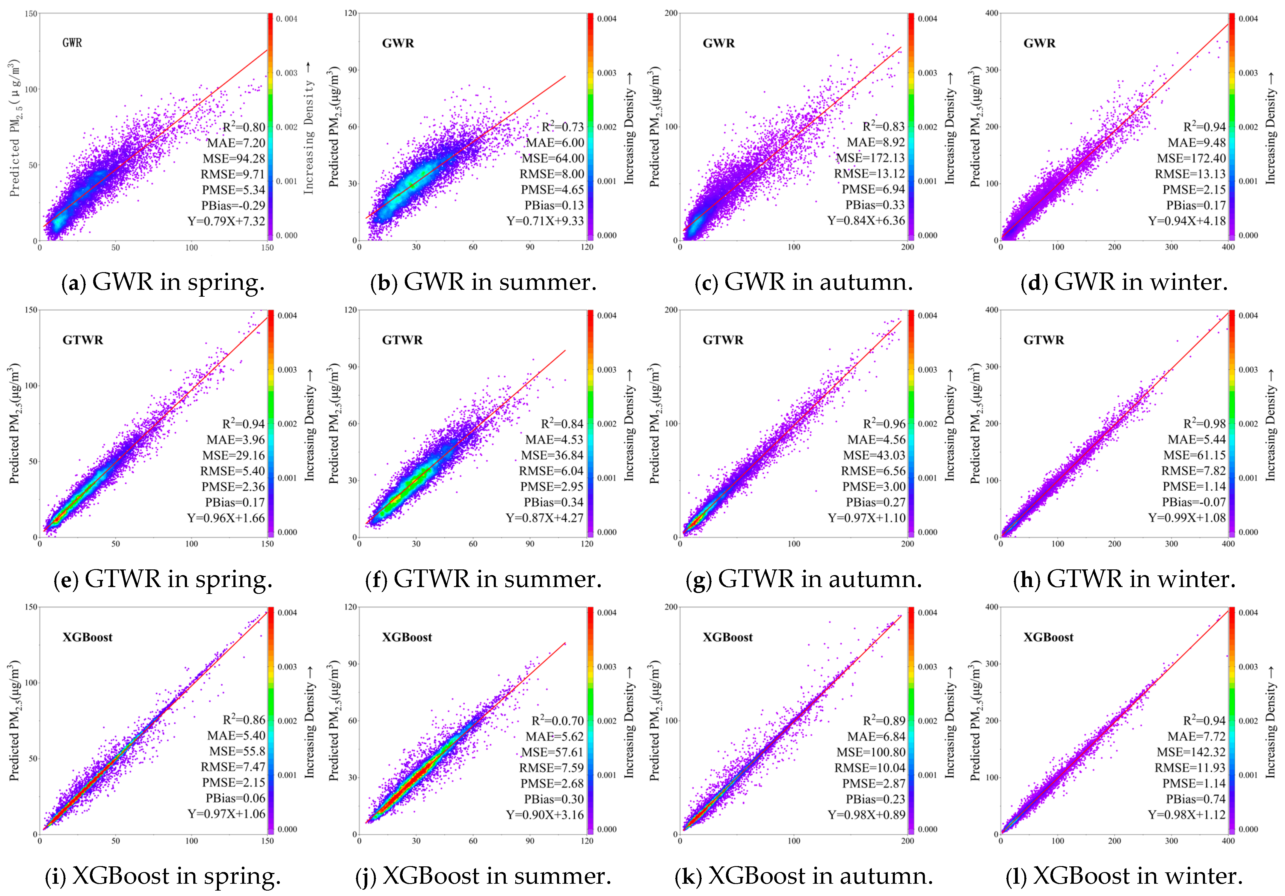
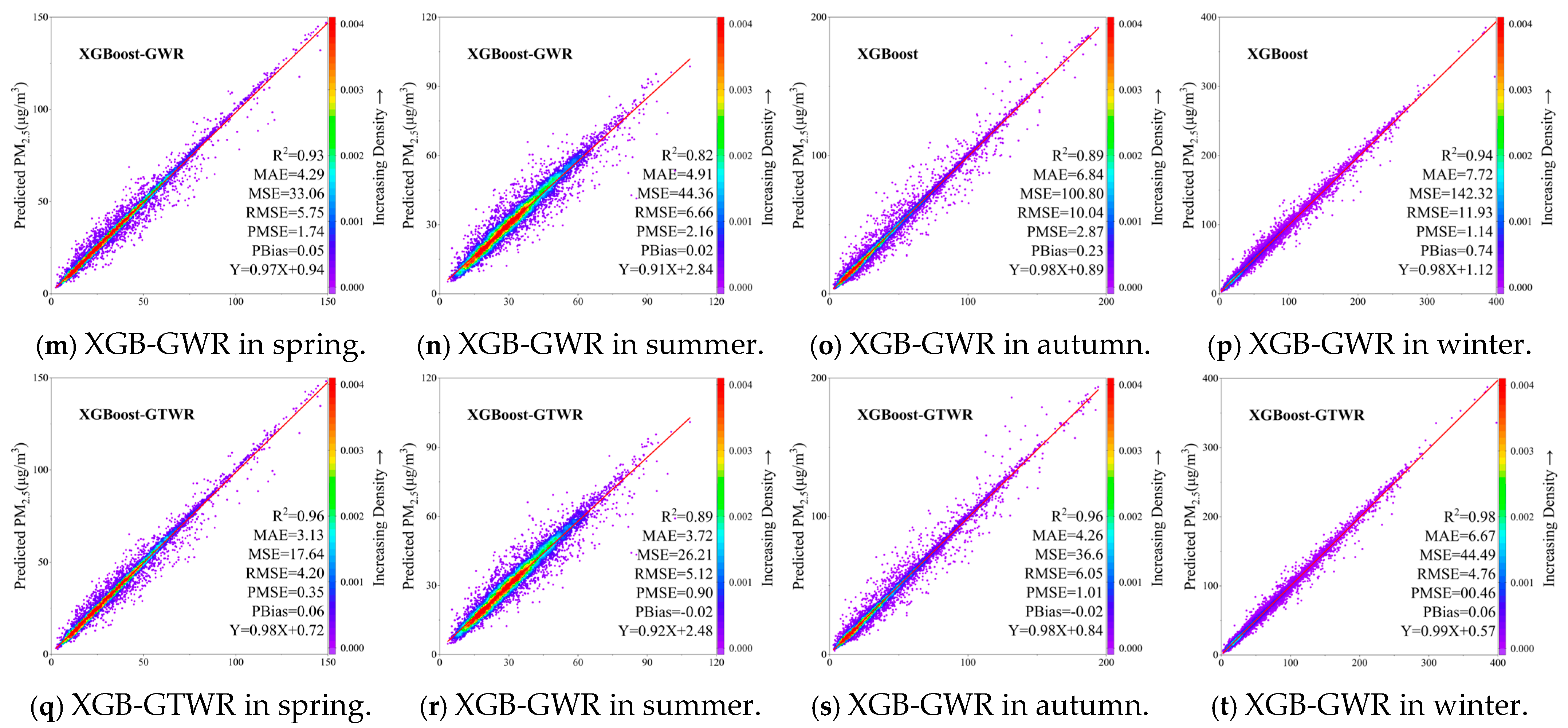
As demonstrated in Figure 4, which presents a scatter plot of the models across four seasons, the accuracy of the GWR, GTWR, XGBoost, XGBoost-GWR, and XGBoost-GTWR models can be more intuitively discerned. It is evident that the lower the prediction accuracy of the GWR model is, the more dispersed the points are in deviating from the fitted curve, and the higher the prediction accuracy of the XGBoost-GTWR model is, the more concentrated the points are in converging to the fitted curve. Furthermore, it was observed that the XGBoost-GTWR model, which demonstrated high prediction accuracy, exhibited a tendency to have a slope that approximated 1 and an intercept that approximated 0. This observation indicates that the predicted value of the PM_2.5 concentration tends to be closer to the observed value. In comparison with the other seasons, winter exhibited the most optimal fit to the fitted curve, with the scatter points in the figure being the closest to the curve overall. Furthermore, the scatter points for the winter season are more clustered around the fitted curve than in the other seasons, indicating a greater tendency for the data to fall within this range.

4.3. Feature Importance and Feature Correlation

To explore the effect of each feature on the prediction of the PM_2.5 concentration, our study was used Pearson’s correlation to assess the prediction results. Pearson correlation analysis refers to the correlation value between each feature and the predicted PM_2.5 concentration. As demonstrated in

Table 11. Pearson correlation coefficients between various features and predicted PM_2.5 concentrations for the quarters and months of 2020.

Time	Features
	PM10	SO2	O3	CO	NO2	dewp	dir	slp	spd	temp	vsb	aod
Spring	0.62	0.32	0.12	0.64	0.55	0.39	−0.30	−0.07	−0.21	0.11	−0.66	0.53
Summer	0.58	0.08	0.22	0.54	0.26	0.32	−0.04	−0.05	−0.03	0.27	−0.58	0.34
Autumn	0.86	0.39	−0.09	0.69	0.74	0.07	−0.08	−0.03	−0.20	−0.05	−0.65	0.50
Winter	0.93	0.27	−0.23	0.79	0.52	0.55	−0.11	−0.13	−0.32	0.32	−0.68	0.34
Jan	0.95	0.19	−0.16	0.75	0.45	0.59	−0.03	−0.05	−0.25	0.35	−0.68	0.40
Feb	0.91	0.14	−0.34	0.78	0.65	0.59	0.05	−0.13	−0.33	0.39	−0.68	0.24
Mar	0.72	0.26	−0.14	0.66	0.55	0.74	−0.30	−0.13	−0.24	0.21	−0.75	0.68
Apr	0.67	0.47	0.40	0.65	0.66	0.76	−0.32	−0.15	−0.31	0.50	−0.62	0.47
May	0.51	0.30	0.34	0.65	0.44	0.54	−0.34	0.04	−0.08	0.20	−0.63	0.43
Jun	0.56	0.16	0.28	0.58	0.33	0.39	−0.09	−0.08	−0.02	0.30	−0.52	0.26
Jul	0.65	−0.04	0.03	0.52	0.10	0.64	−0.01	0.01	−0.10	0.14	−0.64	0.40
Aug	0.82	0.07	0.22	0.62	0.36	0.53	0.09	−0.07	0.01	0.37	−0.58	0.23
Sep	0.84	0.28	0.54	0.61	0.53	0.48	−0.13	−0.09	−0.33	0.07	−0.65	0.59
Oct	0.80	0.39	0.27	0.72	0.71	0.53	−0.17	−0.07	−0.17	0.48	−0.67	0.62
Nov	0.88	0.35	−0.30	0.73	0.75	0.67	−0.14	−0.13	−0.27	0.45	−0.72	0.50
Dec	0.92	0.45	−0.64	0.81	0.76	0.72	−0.35	−0.34	−0.24	0.59	−0.64	0.40

, which presents the Pearson correlation coefficients between each feature and the PM_2.5 prediction value, the correlation between the PM_2.5 concentration and various pollutants is generally positive. This may be because air pollutants are emitted concurrently, with the strongest correlation being observed with PM₁₀. This phenomenon may be attributed to the fact that both categories of particles belong to the fine particulate matter spectrum, with the distinction between them being solely one of particle size. Furthermore, the formation processes of these particles frequently involve the co-emission of particles of various sizes. The correlation with ground-level ozone is weak and exhibits seasonal characteristics, with a positive correlation in autumn and winter and a negative correlation in spring and summer. Regarding the correlation between PM_2.5 concentrations and meteorological factors, a relatively stable and significant negative correlation with visibility (VSB) is evident. This is attributable to the fact that fine particulate matter itself absorbs and reflects light, thereby reducing atmospheric transparency. The findings of the present study demonstrate a strong positive correlation between PM_2.5 concentrations and both the temperature (temp) and thermodynamic humidity parameters, specifically the dew point temperature (dewp). In the humid and hot regions of the Beijing–Tianjin–Hebei area, PM_2.5 concentrations have been observed to be relatively higher. The findings of the present study demonstrate a negative correlation between PM_2.5 concentrations and both wind speed (SPD) and wind direction (DIR), as well as sea-level pressure (SLP). It has been demonstrated that higher wind speeds facilitate the dilution and removal of particulate matter. Regions exhibiting higher atmospheric pressure tend to be characterized by lower elevations, more extensive plains, higher population densities, and greater industrialization. This suggests that the higher PM_2.5 concentrations observed in these regions may not be directly attributable to the atmospheric pressure itself. It is evident from the data that there is a strong positive correlation between PM_2.5 concentrations and AODs, as regions exhibiting elevated aerosol optical depths (AODs) frequently demonstrate higher concentrations of PM_2.5.

4.4. Spatial–Temporal Distribution of Estimated PM_2.5 Concentrations

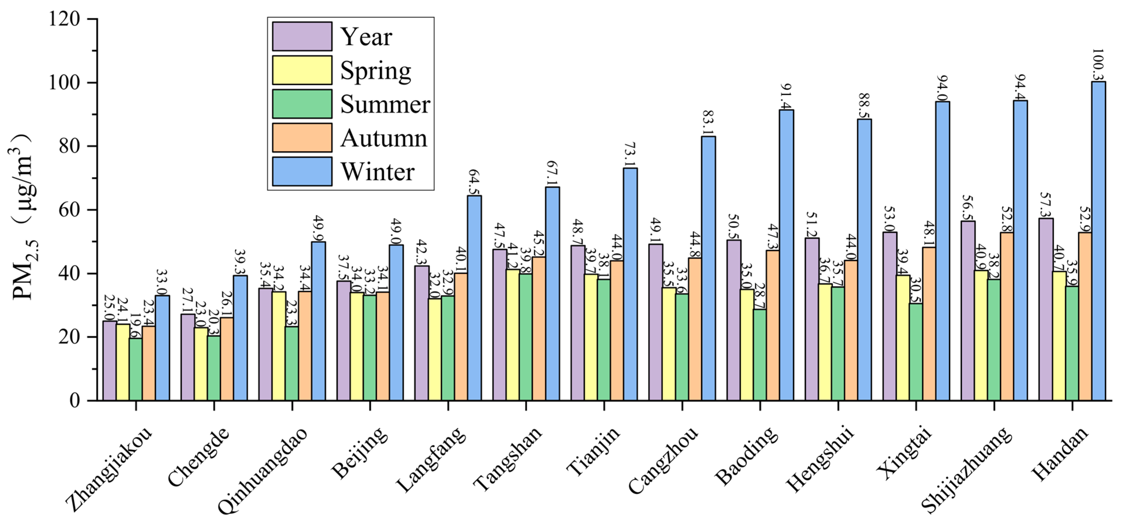
Figure 5 shows the predicted mean annual and seasonal PM_2.5 concentrations for Beijing, Tianjin, and Hebei’s 13 cities, with the cities being arranged in ascending order from left to right based on the annual average PM_2.5 concentration value. The mean PM_2.5 concentrations showed significant spatial variation, with the highest being found in Handan (57.3 μg/m³ annual mean). Regarding seasonal variations, the highest PM_2.5 concentrations were observed in Shijiazhuang during the spring months (40.9 μg/m³), followed by Tangshan in summer (39.8 μg/m³) and Handan in autumn (52.9 μg/m³) and winter (100.3 μg/m³).

The seasonal spatial distribution of the predicted PM_2.5 concentrations is illustrated in Figure 6. The predicted PM_2.5 concentrations were found to be highest in the winter period, with more than half of the regions exhibiting average PM_2.5 concentrations exceeding 70 µg/m³. Conversely, summer exhibited the lowest seasonal PM_2.5 concentration levels throughout the year in the Beijing–Tianjin–Hebei region, with most areas registering average concentrations below 40 μg/m³. The PM_2.5 concentration in the central, southern, and eastern parts of the Beijing–Tianjin–Hebei region is generally higher throughout the year. During the autumn and winter seasons, Handan, Xingtai, Hengshui, Shijiazhuang, Baoding, and Shijiazhuang experienced significantly elevated PM_2.5 concentrations, while Cangzhou, Tianjin, and Tangshan exhibited higher levels. In contrast, other regions demonstrated lower PM_2.5 concentrations. Conversely, in the spring and summer months, Handan, Xingtai, Shijiazhuang, Tianjin, and Tangshan exhibited elevated PM_2.5 concentrations, while other regions demonstrated reduced concentrations.

Among the factors influencing variations in PM_2.5 concentration, the winter combustion peak occurs under conditions of low humidity and low temperature, where sulfide accumulation reaches high concentrations, forming a winter sulfate peak that impacts PM_2.5 levels [54,55]. Nitrates formed from nitrogen oxides decompose more readily in summer’s high temperatures, leading to a summer nitrate “trough”. O₃ does not constitute a component of PM₂.₅; rather, it functions as a potent oxidant, determining the oxidation rates of sulfides, nitrides, and other compounds. A high correlation has been observed between days with elevated O₃ concentrations and elevated secondary inorganic aerosol formation efficiency. CO, functioning as an indicator of incomplete combustion, exerts a significant influence on oxidation capacity through consumption pathways, thereby indirectly promoting secondary particle formation. The substance exhibits synchronous diurnal variations with PM_2.5, yet it does not function as a direct chemical source. It is important to note that high wind speeds do not necessarily result in a decrease in PM_2.5 concentrations. The presence of wind-blown sand and dust may result in concentration rebounds. It has been demonstrated that northerly winds tend to deliver relatively cleaner air, while southerly winds more readily transport polluted air masses.

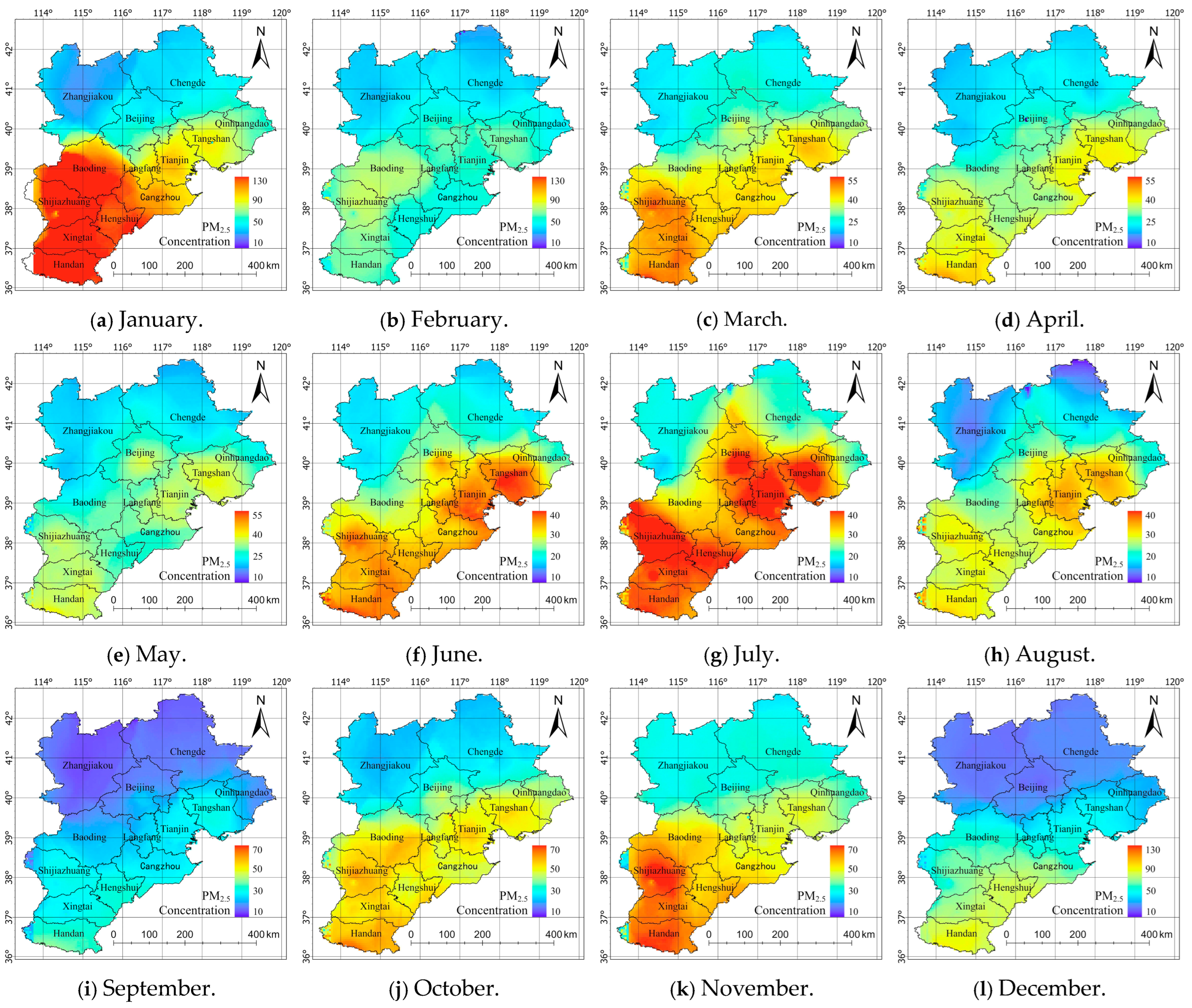
Figure 7 compares the PM_2.5 concentration distribution of each months. In spring, the PM_2.5 concentration decreases gradually from March to May, especially in the southern part of the Beijing–Tianjin–Hebei region. In summer, the PM_2.5 concentration is higher in July than in June and August. In autumn, the PM_2.5 concentration increases from September to November. In winter, the PM_2.5 concentration decreases from January to February, and the high PM_2.5 concentrations in winter are mainly contributed by January.

5. Discussion

Compared with existing studies that either used coarse-resolution AOD products or did not address residual spatial autocorrelation, this study integrates 3 km MODIS AOD with MERRA-2 data and employs a two-stage XGBoost-GTWR hybrid model, achieving higher prediction accuracy (R² = 0.95) while retaining fine spatial granularity. In

Table 12. Comparison between this study and selected previous studies.

Study	Study Area	AOD Source	Spatial Resolution	Model Type	Residual Processing	R2
Zhang et al. (2019) [38]	Guanzhong Basin	VIIRS	6 km	LME + GWR	Nonlinear fusion	0.80
Liu et al. (2023) [36]	Chengdu Chongqing Economic Circle	MODIS	1 km	GTWR + XGBoost	Weak residual modeling	0.92
This study	Jing-Jin-Ji Area	MODIS + MERRA	3 km	XGBoost + GTWR	Spatiotemporal residual correction + nonlinear fusion	0.95

, a comparison is presented between the present study and previous ones.

In addressing the issue of inadequate effective pixels resulting from Aqua AOD cloud gaps, this study employs a fusion algorithm to supplement the missing areas of Aqua using MERRA-2 reanalysis AOD. The results demonstrate that 41.3% of the original missing pixels were successfully filled, and the filled field exhibited significantly improved spatiotemporal continuity in comparison with single-satellite products. Despite the fact that the spatial resolution of MERRA-2 was downsampled from 0.5° to 3 km, its hourly output and completeness characteristics provided a reliable basis for fusion, and the high-resolution details of Aqua were preserved through residual correction. This strategy is intended to ensure the maintenance of the spatial accuracy of satellite products. The model provides continuous, gap-free AOD input for subsequent PM_2.5 estimation, thereby reducing estimation variance caused by data gaps.

The trend in PM_2.5 concentrations across the Beijing–Tianjin–Hebei region demonstrates a gradual decline from January to August, followed by a subsequent gradual increase until December. The highest average concentration recorded in January exceeds the lowest average concentration recorded in August by more than threefold. This is largely attributable to the fact that the southeasterly monsoon in summer facilitates the dispersion of PM_2.5, whereas the northwesterly monsoon in winter is blocked by the Yanshan and Taihang mountain ranges. Furthermore, winter heating exacerbates the accumulation of PM_2.5.

Additionally, RMSE and MAE rise markedly during winter months with high PM_2.5 concentrations; however, this does not indicate a deterioration in model accuracy. As absolute-error metrics, RMSE and MAE scale linearly with the ambient concentration itself. Consequently, even when the relative error remains unchanged, their values increase in proportion to the elevated winter concentrations. Relying solely on RMSE or MAE to evaluate performance across months with vastly different magnitudes (e.g., January vs. August) can therefore lead to the erroneous conclusion that “winter predictions are worse” [37,56,57,58]. To eliminate this scale effect, we introduced the dimensionless PMSE (%MSE), which normalizes errors to a percentage scale and enables a fair comparison of true model accuracy across seasons and pollution levels.

The spatial pattern of PM_2.5 in the Beijing–Tianjin–Hebei region, characterized by higher concentrations in the south than in the north, is the result of a combination of emissions, topography and meteorology. The central-southern plains (Shijiazhuang, Xingtai, Handan and Hengshui) are characterized by an elevation of less than 50 meters, elevated levels of industrial and transport emissions, and semi-enclosed ‘dustpan’ topography, which is bordered by the Taihang Mountains to the west and the Bohai Sea to the east. This configuration gives rise to frequent winter stagnation and the facile accumulation of pollutants. Conversely, the northern mountainous plateau regions (Zhangjiakou, Chengde and north-west Beijing) have elevations in excess of 800 m, sparse populations and low emission baselines. These regions are distinguished by the presence of intense turbulence and conducive dispersion conditions. The coastal industrial belt, comprising Tianjin, Tangshan and Cangzhou, is distinguished by its flat terrain, yet it is notable for its dense port transportation infrastructure and significant presence of heavy chemical industries. The presence of significant secondary aerosol formation in this area is attributable to the combination of sea–land breeze circulation, thus classifying it within the second tier of concentration levels. Despite having the highest population density, urban areas in Beijing have experienced a significant decrease in primary emission factors since 2013. This decline can be attributed to strict measures such as the conversion of coal-fired power plants to electricity, the crackdown on scattered, disorderly and polluting enterprises, and stricter vehicle emission standards. Consequently, the average PM_2.5 concentration in Beijing is now 30–50 μg/m³ lower than in southern plain cities, which highlights the decisive role of emission reduction policies in local concentration levels.

6. Conclusions

This study presents a novel two-stage framework that integrates a machine learning model (XGBoost) with a spatial–temporal regression model (GTWR) to estimate daily PM_2.5 concentrations in the Beijing–Tianjin–Hebei region at a fine spatial resolution of 3 km. Compared with previous studies, the main innovations are as follows: high-resolution AOD fusion strategy combining MODIS Collection 6.1 (3 km) with MERRA-2 background data, improving both data completeness and spatial coverage; residual correction mechanism where GTWR explicitly models the spatiotemporal autocorrelation of prediction residuals from XGBoost, enhancing robustness and accuracy; and comprehensive model evaluation across monthly and seasonal time scales, confirming that the proposed XGBoost–GTWR model outperforms traditional single-stage and hybrid models (R² = 0.95). These innovations offer a generalizable framework for fine-scale air pollution estimation in data-scarce or topographically complex regions.

This research still has some shortcomings and areas for future work. First at all, the current feature set only includes natural factors, such as meteorology, pollutants and remote sensing data. As anthropogenic emission information is indirectly reflected through natural variables, it is difficult to attribute PM_2.5 concentrations directly to either natural or anthropogenic drivers directly. Future work will introduce socioeconomic indicators in order to construct a dual natural–anthropogenic feature space. This will enable the explicit quantification and attribution analysis of emission source contributions. Secondly, the study used one year of data to predict PM_2.5 concentrations and was unable to explore the interannual variation patterns of PM_2.5 concentration. Using continuous years of meteorological and pollutant observation data to predict PM_2.5 concentration can explore the annual variation pattern of PM_2.5 concentration and further explore the monthly year-on-year variation pattern.

References

1. Liu, J.; Kiesewetter, G.; Klimont, Z.; Cofala, J.; Heyes, C.; Schöpp, W.; Zhu, T.; Cao, G.; Gomez Sanabria, A.; Sander, R.; et al. Mitigation Pathways of Air Pollution from Residential Emissions in the Beijing-Tianjin-Hebei Region in China. Environ. Int. 2019, 125, 236–244. [Google Scholar] [CrossRef]
2. Apte, J.S.; Brauer, M.; Cohen, A.J.; Ezzati, M.; Pope, C.A. Ambient PM2.5 Reduces Global and Regional Life Expectancy. Environ. Sci. Technol. Lett. 2018, 5, 546–551. [Google Scholar] [CrossRef]
3. Krittanawong, C.; Qadeer, Y.K.; Hayes, R.B.; Wang, Z.; Thurston, G.D.; Virani, S.; Lavie, C.J. PM2.5 and Cardiovascular Diseases: State-of-the-Art Review. Int. J. Cardiol. Cardiovasc. Risk Prev. 2023, 19, 200217. [Google Scholar] [CrossRef]
4. Xie, C.; Xia, X.; Wang, K.; Yan, J.; Bai, L.; Guo, L.; Li, X.; Wu, S. Ambient Air Pollution and Parkinson’s Disease and Alzheimer’s Disease: An Updated Meta-Analysis. Toxics 2025, 13, 139. [Google Scholar] [CrossRef]
5. Amnuaylojaroen, T.; Kaewkanchanawong, P.; Panpeng, P. Distribution and Meteorological Control of PM2.5 and Its Effect on Visibility in Northern Thailand. Atmosphere 2023, 14, 538. [Google Scholar] [CrossRef]
6. Wu, H.; Cao, Y.; Wang, T.; You, J.; Yang, T.; Qu, Y.; Yan, S.; Yang, H.; Mu, X.; Gao, L.; et al. How Does PM2.5 Impact the Urban Vertical Temperature Structure? A Case Study in Nanjing. Aerosol Air Qual. Res. 2024, 24, 230214. [Google Scholar] [CrossRef]
7. Zhou, L.; Chen, X.; Tian, X. The Impact of Fine Particulate Matter (PM2.5) on China’s Agricultural Production from 2001 to 2010. J. Clean. Prod. 2018, 178, 133–141. [Google Scholar] [CrossRef]
8. Saha, D.; Pandya, A.; Singh, J.K.; Paswan, S.; Singh, D.D.N. Role of Environmental Particulate Matters on Corrosion of Copper. Atmos. Pollut. Res. 2016, 7, 1037–1042. [Google Scholar] [CrossRef]
9. Chen, G.; Morawska, L.; Zhang, W.; Li, S.; Cao, W.; Ren, H.; Wang, B.; Wang, H.; Knibbs, L.D.; Williams, G.; et al. Spatiotemporal Variation of PM1 Pollution in China. Atmos. Environ. 2018, 178, 198–205. [Google Scholar] [CrossRef]
10. Martin, R.V.; Brauer, M.; Van Donkelaar, A.; Shaddick, G.; Narain, U.; Dey, S. No One Knows Which City Has the Highest Concentration of Fine Particulate Matter. Atmos. Environ. X 2019, 3, 100040. [Google Scholar] [CrossRef]
11. Wang, J.; Christopher, S.A. Intercomparison between Satellite-derived Aerosol Optical Thickness and PM2.5 Mass: Implications for Air Quality Studies. Geophys. Res. Lett. 2003, 30. [Google Scholar] [CrossRef]
12. Christopher, S.; Gupta, P. Global Distribution of Column Satellite Aerosol Optical Depth to Surface PM2.5 Relationships. Remote Sens. 2020, 12, 1985. [Google Scholar] [CrossRef]
13. Tian, Z.; Wei, J.; Li, Z. How Important Is Satellite-Retrieved Aerosol Optical Depth in Deriving Surface PM2.5 Using Machine Learning? Remote Sens. 2023, 15, 3780. [Google Scholar] [CrossRef]
14. Liu, Y.; Sarnat, J.A.; Kilaru, V.; Jacob, D.J.; Koutrakis, P. Estimating Ground-Level PM2.5 in the Eastern United States Using Satellite Remote Sensing. Environ. Sci. Technol. 2005, 39, 3269–3278. [Google Scholar] [CrossRef] [PubMed]
15. Remer, L.A.; Kaufman, Y.J.; Tanré, D.; Mattoo, S.; Chu, D.A.; Martins, J.V.; Li, R.-R.; Ichoku, C.; Levy, R.C.; Kleidman, R.G.; et al. The MODIS Aerosol Algorithm, Products, and Validation. J. Atmos. Sci. 2005, 62, 947–973. [Google Scholar] [CrossRef]
16. Buchard, V.; Randles, C.A.; Da Silva, A.M.; Darmenov, A.; Colarco, P.R.; Govindaraju, R.; Ferrare, R.; Hair, J.; Beyersdorf, A.J.; Ziemba, L.D.; et al. The MERRA-2 Aerosol Reanalysis, 1980 Onward. Part II: Evaluation and Case Studies. J. Clim. 2017, 30, 6851–6872. [Google Scholar] [CrossRef]
17. Guo, B.; Wang, Z.; Pei, L.; Zhu, X.; Chen, Q.; Wu, H.; Zhang, W.; Zhang, D. Reconstructing MODIS Aerosol Optical Depth and Exploring Dynamic and Influential Factors of AOD via Random Forest at the Global Scale. Atmos. Environ. 2023, 315, 120159. [Google Scholar] [CrossRef]
18. Cui, Q.; Zhang, F.; Fu, S.; Wei, X.; Ma, Y.; Wu, K. High Spatiotemporal Resolution PM2.5 Concentration Estimation with Machine Learning Algorithm: A Case Study for Wildfire in California. Remote Sens. 2022, 14, 1635. [Google Scholar] [CrossRef]
19. Geng, G.; Zhang, Q.; Martin, R.V.; Van Donkelaar, A.; Huo, H.; Che, H.; Lin, J.; He, K. Estimating Long-Term PM2.5 Concentrations in China Using Satellite-Based Aerosol Optical Depth and a Chemical Transport Model. Remote Sens. Environ. 2015, 166, 262–270. [Google Scholar] [CrossRef]
20. Jing, Y.; Pan, L.; Sun, Y. Estimating PM2.5 Concentrations in a Central Region of China Using a Three-Stage Model. Int. J. Digit. Earth 2023, 16, 578–592. [Google Scholar] [CrossRef]
21. Wu, J.; Winer, A.M.; Delfino, R.J. Exposure Assessment of Particulate Matter Air Pollution before, during, and after the 2003 Southern California Wildfires. Atmos. Environ. 2006, 40, 3333–3348. [Google Scholar] [CrossRef]
22. Neupane, B.; Jerrett, M.; Burnett, R.T.; Marrie, T.; Arain, A.; Loeb, M. Long-Term Exposure to Ambient Air Pollution and Risk of Hospitalization with Community-Acquired Pneumonia in Older Adults. Am. J. Respir. Crit. Care Med. 2010, 181, 47–53. [Google Scholar] [CrossRef]
23. Jerrett, M.; Burnett, R.T.; Ma, R.; Pope, C.A.; Krewski, D.; Newbold, K.B.; Thurston, G.; Shi, Y.; Finkelstein, N.; Calle, E.E.; et al. Spatial Analysis of Air Pollution and Mortality in Los Angeles. Epidemiology 2005, 16, 727–736. [Google Scholar] [CrossRef] [PubMed]
24. Lu, G.Y.; Wong, D.W. An Adaptive Inverse-Distance Weighting Spatial Interpolation Technique. Comput. Geosci. 2008, 34, 1044–1055. [Google Scholar] [CrossRef]
25. Brunsdon, C.; Fotheringham, A.S.; Charlton, M.E. Geographically Weighted Regression: A Method for Exploring Spatial Nonstationarity. Geogr. Anal. 1996, 28, 281–298. [Google Scholar] [CrossRef]
26. Bai, Y.; Wu, L.; Qin, K.; Zhang, Y.; Shen, Y.; Zhou, Y. A Geographically and Temporally Weighted Regression Model for Ground-Level PM2.5 Estimation from Satellite-Derived 500 m Resolution AOD. Remote Sens. 2016, 8, 262. [Google Scholar] [CrossRef]
27. Hu, X.; Waller, L.A.; Al-Hamdan, M.Z.; Crosson, W.L.; Estes, M.G.; Estes, S.M.; Quattrochi, D.A.; Sarnat, J.A.; Liu, Y. Estimating Ground-Level PM2.5 Concentrations in the Southeastern U.S. Using Geographically Weighted Regression. Environ. Res. 2013, 121, 1–10. [Google Scholar] [CrossRef] [PubMed]
28. Yu, X.; Lary, D.J.; Simmons, C.S. PM2.5 Modeling and Historical Reconstruction over the Continental USA Utilizing GOES-16 AOD. Remote Sens. 2021, 13, 4788. [Google Scholar] [CrossRef]
29. Gu, J.; Wang, Y.; Ma, J.; Lu, Y.; Wang, S.; Li, X. An Estimation Method for PM2.5 Based on Aerosol Optical Depth Obtained from Remote Sensing Image Processing and Meteorological Factors. Remote Sens. 2022, 14, 1617. [Google Scholar] [CrossRef]
30. He, W.; Zhang, S.; Meng, H.; Han, J.; Zhou, G.; Song, H.; Zhou, S.; Zheng, H. Full-Coverage PM2.5 Mapping and Variation Assessment during the Three-Year Blue-Sky Action Plan Based on a Daily Adaptive Modeling Approach. Remote Sens. 2022, 14, 3571. [Google Scholar] [CrossRef]
31. Kulkarni, P.; Sreekanth, V.; Upadhya, A.R.; Gautam, H.C. Which model to choose? Performance comparison of statistical and machine learning models in predicting PM2.5 from high-resolution satellite aerosol optical depth. Atmos. Environ. 2022, 282, 119164. [Google Scholar] [CrossRef]
32. Peng, J.; Han, H.; Yi, Y.; Huang, H.; Xie, L. Machine learning and deep learning modeling and simulation for predicting PM2.5 concentrations. Chemosphere 2022, 308, 136353. [Google Scholar] [CrossRef]
33. Liu, N.; Hao, Z.; Zhao, P. Spatiotemporal change of PM2.5 concentration in Beijing-Tianjin-Hebei and its prediction based on machine learning. Urban Clim. 2024, 58, 102167. [Google Scholar] [CrossRef]
34. Tian, Y.; Zhang, Y. A Comprehensive Survey on Regularization Strategies in Machine Learning. Inf. Fusion 2022, 80, 146–166. [Google Scholar] [CrossRef]
35. Zhang, C.; Bengio, S.; Hardt, M.; Recht, B.; Vinyals, O. Understanding Deep Learning (Still) Requires Rethinking Generalization. Commun. ACM 2021, 64, 107–115. [Google Scholar] [CrossRef]
36. Liu, M.; Luo, X.; Qi, L.; Liao, X.; Chen, C. Simulation of the Spatiotemporal Distribution of PM2.5 Concentration Based on GTWR-XGBoost Two-Stage Model: A Case Study of Chengdu Chongqing Economic Circle. Atmosphere 2023, 14, 115. [Google Scholar] [CrossRef]
37. Chen, X.; Zhang, W.; He, J.; Zhang, L.; Guo, H.; Li, J.; Gu, X. Mapping PM2.5 Concentration from the Top-of-Atmosphere Reflectance of Himawari-8 via an Ensemble Stacking Model. Atmos. Environ. 2024, 330, 120560. [Google Scholar] [CrossRef]
38. Zhang, K.; De Leeuw, G.; Yang, Z.; Chen, X.; Su, X.; Jiao, J. Estimating Spatio-Temporal Variations of PM2.5 Concentrations Using VIIRS-Derived AOD in the Guanzhong Basin, China. Remote Sens. 2019, 11, 2679. [Google Scholar] [CrossRef]
39. Chen, C.-C.; Wang, Y.-R.; Yeh, H.-Y.; Lin, T.-H.; Huang, C.-S.; Wu, C.-F. Estimating Monthly PM2.5 Concentrations from Satellite Remote Sensing Data, Meteorological Variables, and Land Use Data Using Ensemble Statistical Modeling and a Random Forest Approach. Environ. Pollut. 2021, 291, 118159. [Google Scholar] [CrossRef]
40. Bera, B.; Bhattacharjee, S.; Sengupta, N.; Saha, S. PM2.5 Concentration Prediction during COVID-19 Lockdown over Kolkata Metropolitan City, India Using MLR and ANN Models. Environ. Chall. 2021, 4, 100155. [Google Scholar] [CrossRef]
41. Comber, A. Hyper-Local Geographically Weighted Regression: Extending GWR through Local Model Selection and Local Bandwidth Optimization. J. Spat. Inf. Sci. 2018, 17, 63–84. [Google Scholar] [CrossRef]
42. Chen, T.; Guestrin, C. XGBoost: A Scalable Tree Boosting System. In Proceedings of the 22nd ACM SIGKDD International Conference on Knowledge Discovery and Data Mining, San Francisco, CA, USA, 13–17 August 2016; pp. 785–794. [Google Scholar]
43. Xue, T.; Zheng, Y.; Geng, G.; Zheng, B.; Jiang, X.; Zhang, Q.; He, K. Fusing Observational, Satellite Remote Sensing and Air Quality Model Simulated Data to Estimate Spatiotemporal Variations of PM2.5 Exposure in China. Remote Sens. 2017, 9, 221. [Google Scholar] [CrossRef]
44. Wei, J.; Huang, W.; Li, Z.; Xue, W.; Peng, Y.; Sun, L.; Cribb, M. Estimating 1-Km-Resolution PM2.5 Concentrations across China Using the Space-Time Random Forest Approach. Remote Sens. Environ. 2019, 231, 111221. [Google Scholar] [CrossRef]
45. Widya, L.K.; Hsu, C.-Y.; Lee, H.-Y.; Jaelani, L.M.; Lung, S.-C.C.; Su, H.-J.; Wu, C.-D. Comparison of Spatial Modelling Approaches on PM10 and NO2 Concentration Variations: A Case Study in Surabaya City, Indonesia. Int. J. Environ. Res. Public Health 2020, 17, 8883. [Google Scholar] [CrossRef]
46. Moriasi, D.N.; Arnold, J.G.; Van Liew, M.W.; Bingner, R.L.; Harmel, R.D.; Veith, T.L. Model Evaluation Guidelines for Systematic Quantification of Accuracy in Watershed Simulations. Trans. ASABE 2007, 50, 885–900. [Google Scholar] [CrossRef]
47. Hu, K.; Guo, Y.; Hu, D.; Du, R.; Yang, X.; Zhong, J.; Fei, F.; Chen, F.; Chen, G.; Zhao, Q.; et al. Mortality Burden Attributable to PM1 in Zhejiang Province, China. Environ. Int. 2018, 121, 515–522. [Google Scholar] [CrossRef] [PubMed]
48. Wong, P.-Y.; Lee, H.-Y.; Chen, Y.-C.; Zeng, Y.-T.; Chern, Y.-R.; Chen, N.-T.; Candice Lung, S.-C.; Su, H.-J.; Wu, C.-D. Using a Land Use Regression Model with Machine Learning to Estimate Ground Level PM2.5. Environ. Pollut. 2021, 277, 116846. [Google Scholar] [CrossRef]
49. Baron, G.; Stańczyk, U. Standard vs. Non-Standard Cross-Validation: Evaluation of Performance in a Space with Structured Distribution of Datapoints. Procedia Comput. Sci. 2021, 192, 1245–1254. [Google Scholar] [CrossRef]
50. GB 3095-2012; Ministry of Environmental Protection. Ambient Air Quality Standards. Environmental Science Press: Beijing, China, 2012.
51. WHO. WHO Global Air Quality Guidelines: Particulate Matter (PM2.5 and PM10), Ozone, Nitrogen Dioxide, Sulfur Dioxide and Carbon Monoxide; World Health Organization: Geneva, Switzerland, 2021; ISBN 978-92-4-003422-8. Available online: https://apps.who.int/iris/handle/10665/345329 (accessed on 19 September 2025).
52. Jandacka, D.; Durcanska, D.; Nicolanska, M.; Holubcik, M. Impact of Seasonal Heating on PM10 and PM2.5 Concentrations in Sučany, Slovakia: A Temporal and Spatial Analysis. Fire 2024, 7, 150. [Google Scholar] [CrossRef]
53. Jandacka, D.; Durcanska, D. Seasonal Variation, Chemical Composition, and PMF-Derived Sources Identification of Traffic-Related PM1, PM2.5, and PM2.5–10 in the Air Quality Management Region of Žilina, Slovakia. Int. J. Environ. Res. Public Health 2021, 18, 10191. [Google Scholar] [CrossRef]
54. Shikhovtsev, M.Y.; Makarov, M.M.; Aslamov, I.A.; Tyurnev, I.N.; Molozhnikova, Y.V. Application of Modern Low-Cost Sensors for Monitoring of Particle Matter in Temperate Latitudes: An Example from the Southern Baikal Region. Sustainability 2025, 17, 3585. [Google Scholar] [CrossRef]
55. Shikhovtsev, M.Y.; Molozhnikova, Y.V.; Obolkin, V.A.; Potemkin, V.L.; Lutskin, E.S.; Khodzher, T.V. Features of Temporal Variability of the Concentrations of Gaseous Trace Pollutants in the Air of the Urban and Rural Areas in the Southern Baikal Region (East Siberia, Russia). Appl. Sci. 2024, 14, 8327. [Google Scholar] [CrossRef]
56. Dong, L.; Li, S.; Xing, J.; Lin, H.; Wang, S.; Zeng, X.; Qin, Y. Joint Features Random Forest (JFRF) Model for Mapping Hourly Surface PM2.5 over China. Atmos. Environ. 2022, 273, 118969. [Google Scholar] [CrossRef]
57. Sun, Y.; Xue, Y.; Jiang, X.; Jin, C.; Wu, S.; Zhou, X. Estimation of the PM2.5 and PM10 Mass Concentration over Land from FY-4A Aerosol Optical Depth Data. Remote Sens. 2021, 13, 4276. [Google Scholar] [CrossRef]
58. Chu, W.; Zhang, C.; Zhao, Y.; Li, R.; Wu, P. Spatiotemporally Continuous Reconstruction of Retrieved PM2.5 Data Using an Autogeoi-Stacking Model in the Beijing-Tianjin-Hebei Region, China. Remote Sens. 2022, 14, 4432. [Google Scholar] [CrossRef]
Figure 1. Geographical location, urban background environmental air quality monitoring stations.
Atmosphere 16 01300 g001
Figure 2. The technological procedure of two-stage models in the study.
Atmosphere 16 01300 g002
Figure 3. Yearly, monthly and daily variation in average PM2.5 concentration in Beijing–Tianjin–Hebei region in 2020.
Atmosphere 16 01300 g003
Figure 4. Prediction performance of the models: GWR (ad), GTWR (eh), XGBoost (il), XGBoost-GWR (mp), and XGBoost-GTWR (qt). The observed PM2.5 concentration denotes the ground-measured PM2.5 concentration from monitoring sites in 2020, and the predicted PM2.5 concentration reflects the simulated PM2.5 concentration from five models. The red lines denote the best-fitting regression lines for the four machine learning models, and the shaded color represents the density of the samples.
Atmosphere 16 01300 g004aAtmosphere 16 01300 g004b
Figure 5. Mean annual and seasonal variation in predicted PM2.5 concentration for each city in the Beijing–Tianjin–Hebei region in 2020.
Atmosphere 16 01300 g005
Figure 6. Spatial distribution of predicted PM2.5 concentrations in the Beijing–Tianjin–Hebei region for each quarter in 2020: (a) spring, (b) summer, (c) autumn, and (d) winter.
Atmosphere 16 01300 g006
Figure 7. Spatial distribution of predicted PM2.5 concentrations in the Beijing–Tianjin–Hebei region for each quarter and month in 2020.
Atmosphere 16 01300 g007