Hybrid Deep Learning Models for Predicting Meteorological Variables Associated with Santa Ana Wind Conditions in the Guadalupe Basin

Abstract

Santa Ana winds are extreme meteorological events that strongly affect the U.S.–Mexico border region, often associated with droughts, high fire risk, and hydrological imbalance. Understanding the temporal behavior of key atmospheric variables during these events is crucial for integrated water resource management in semi-arid regions such as the Guadalupe Basin in northern Baja California. In this study, we explored the predictive capability of several hybrid deep learning architectures—Long Short-Term Memory (LSTM), Convolutional Neural Network combined with LSTM (CNN–LSTM), and Bidirectional LSTM with Attention (BiLSTM–Attention)—to model the temporal evolution of wind speed, wind direction, temperature, relative humidity, and atmospheric pressure using Modern-Era Retrospective analysis for Research and Applications, Version 2 (MERRA-2) reanalysis data from 1980 to 2020. Model performance was evaluated using RMSE, MAE, and R² metrics and compared against persistence and climatology baselines. The BiLSTM–Attention model achieved the best overall performance, showing particularly high accuracy for temperature (R² = 0.95) and relative humidity (R² = 0.76), while maintaining angular errors below 35° for wind direction. The results demonstrate the potential of hybrid deep learning models to capture nonlinear temporal dependencies in meteorological time series and provide a methodological framework to enhance hydrometeorological understanding and water resource management in the Guadalupe Basin under Santa Ana wind conditions.

1. Introduction

Santa Ana winds are a recurrent meteorological phenomenon that affect the southwestern United States and northwestern Mexico, particularly during fall and winter [1,2,3,4]. These warm, dry Föhn-type winds originate in the Great Basin and blow toward the Pacific coast, typically occurring between September and April, with maximum frequency between October and December [5,6,7]. Their intensity, duration, and direction strongly influence regional climate, fire regimes, and air quality across southern California and northern Baja California. Moreover, ocean–atmosphere interactions in adjacent regions, such as the Gulf of California, also modulate regional climate dynamics and the transport of mineral dust [8], underscoring the complex interplay between atmospheric and surface processes in northwestern Mexico.

The climatology of Santa Ana winds has been primarily investigated through synoptic-scale analyses and mesoscale modeling approaches [2,3,4,9,10]. Classical diagnostic approaches such as Raphael’s pressure-field analysis and the Fire Weather Index classification by Jones et al. have improved the conceptual understanding of these events [3,11]. However, most existing models rely on coarse-resolution atmospheric data from reanalysis or forecast systems such as NCEP–DOE, NAM, RUC, or WRF [12,13], which struggle to reproduce local variability due to the region’s complex topography and heterogeneous surface conditions [14]. Furthermore, conventional numerical weather prediction models often face challenges in accurately capturing the timing and intensity of rapidly evolving atmospheric processes because of the nonlinear nature of the governing equations [15]. These limitations highlight the need for more flexible, data-driven frameworks capable of representing local atmospheric dynamics with lower computational cost.

The Santa Ana winds are a key component of the regional climate and play a crucial role in fire ecology, agriculture, and socioeconomic stability in northwestern Mexico. Their combination of strong gusts, low humidity, and warm temperatures promotes rapid fire spread, causing significant damage to infrastructure, ecosystems, and human health [16,17]. Accurate forecasting of these events is therefore essential for wildfire prevention, agricultural management, and water resource planning. Reliable short-term forecasts can support irrigation scheduling, pest control, and risk reduction, helping to optimize agricultural practices and improve adaptation to climate variability [18]. In water-limited regions such as the Guadalupe Basin, meteorological forecasting is also vital for efficient water allocation and climate risk management in agriculture and tourism.

Recent advances in machine learning (ML) have opened new opportunities for predicting complex meteorological phenomena. Neural network-based methods have been successfully applied to forecast large-scale climate variability, such as the El Niño–Southern Oscillation [19], and to predict key atmospheric variables including precipitation [20], evapotranspiration [19], temperature [21,22], and wind speed [23,24,25,26,27,28,29,30,31]. Among these, Long Short-Term Memory (LSTM) networks have shown superior ability to capture nonlinear and long-term temporal dependencies [32]. For instance, Alves et al. [14] reported that LSTM models achieved mean absolute errors below the minimum accuracy threshold defined by the World Meteorological Organization (WMO), while hybrid architectures combining deep learning techniques—such as Extreme Learning Machine–Online Regularized Extreme Learning Machine–Deep Belief Network (ELM–ORELM–DBN), Ensemble Empirical Mode Decomposition–Long Short-Term Memory (EEMD–LSTM)and Convolutional Neural Network–Long Short-Term Memory (CNN–LSTM)—have demonstrated enhanced predictive performance [33,34,35]. These findings highlight the robustness of hybrid and deep learning models for atmospheric time series forecasting.

Despite recent advances in the application of deep learning to meteorological forecasting, few studies have explored its potential to model the dynamics of Santa Ana wind conditions or their associated climatic context in northwestern Mexico. This study addresses that gap by evaluating multiple hybrid deep learning architectures—including LSTM, CNN–LSTM, and BiLSTM with Attention—to predict five key meteorological variables—wind speed, wind direction, temperature, relative humidity, and atmospheric pressure—in the Guadalupe Basin, Baja California. These variables are essential for identifying and characterizing Santa Ana events and understanding their broader climatic implications. By integrating a data-driven predictive framework with multifractal analysis, this research provides new insights into the temporal complexity of regional atmospheric dynamics and supports the development of early-warning tools for integrated water resource management and climate adaptation in the Guadalupe Basin.

2. Materials and Methods

2.1. Area of Study

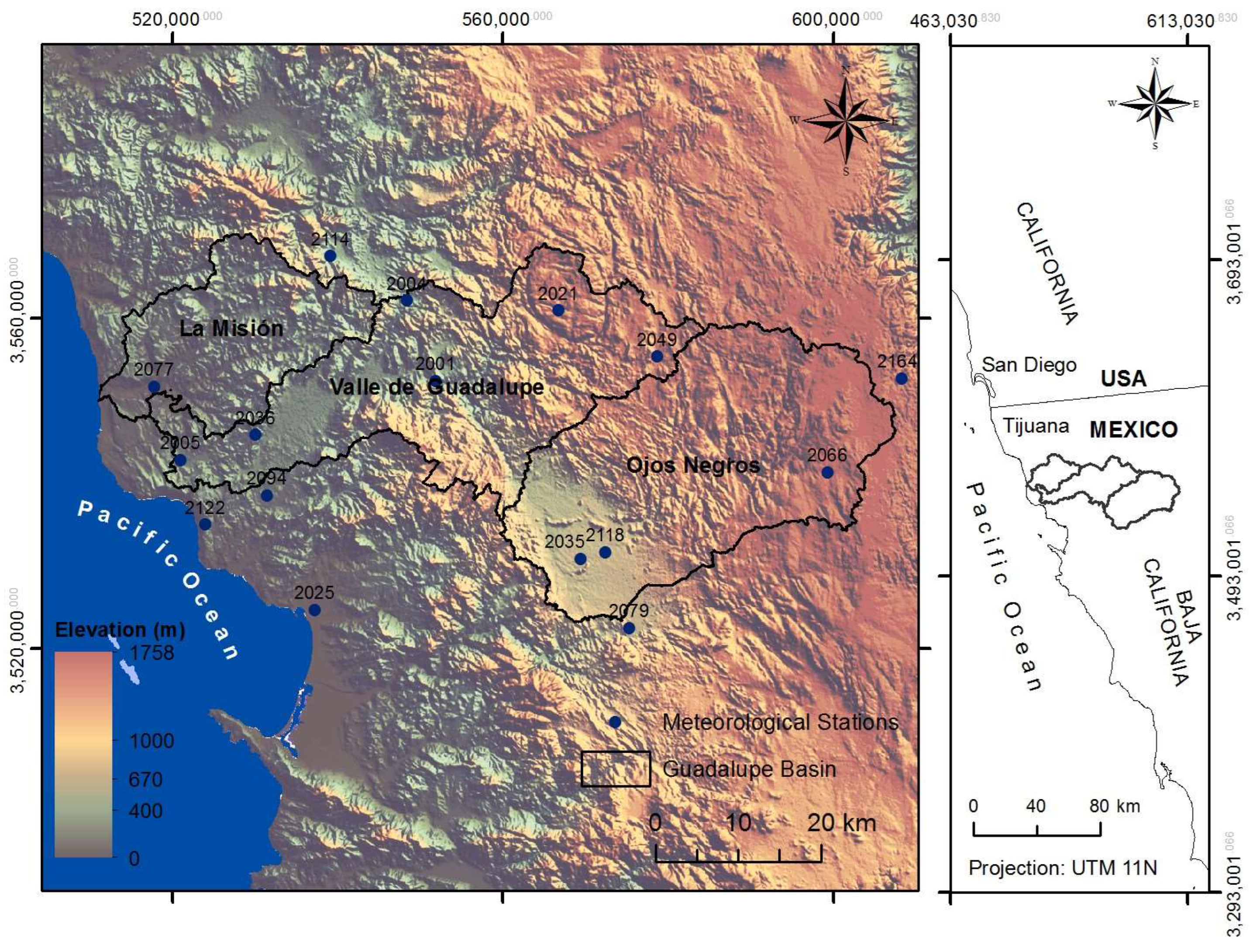
The study was conducted in the Guadalupe Basin, located in northwestern Baja California, Mexico. The basin includes three main valleys—Ojos Negros, Guadalupe, and La Misión—and represents one of the most productive agricultural areas in the region, with the Valle de Guadalupe sub-basin being well known for its viticultural potential. Meteorological data were extracted from the grid cell corresponding to the Agua Caliente station (station code 2021; 32.110° N, −116.450° W), which was selected as a representative location for the basin’s central climatic conditions (Figure 1) [36].

2.2. Data Sources and Preprocessing

The meteorological data used in this study were obtained from the Modern-Era Retrospective Analysis for Research and Applications, Version 2 (MERRA-2) reanalysis dataset for the period 1980–2020. The grid cell corresponding to the Agua Caliente station (latitude 32.110° N, longitude −116.450° W) was selected as the reference point for the Guadalupe Basin, located in northern Baja California, Mexico. This basin encompasses the Ojos Negros, Valle de Guadalupe, and La Misión valleys, which are among the most productive agricultural areas in the region and are of high economic importance due to their viticultural potential.

The MERRA-2 dataset provides continuous and spatially homogeneous records of wind speed, wind direction, temperature, relative humidity, and atmospheric pressure with a daily temporal resolution. The data were divided into training (70%), validation (15%), and testing (15%) subsets to ensure proper model generalization.

Although in situ observations from the Agua Caliente station (CONAGUA network) were available, their limited temporal coverage (2009–2020), lack of continuity, and incomplete set of meteorological variables—restricted mainly to precipitation and temperature—made them unsuitable for deep learning training or validation. Therefore, they were used only for descriptive comparison and consistency verification with the MERRA-2 climatology.

Prior to model training, all variables were normalized using a Min–Max scaler in the range [0, 1] to enhance numerical stability during the learning process. Additionally, wind direction was decomposed into its sine and cosine components to avoid discontinuities associated with angular values (e.g., 0° and 360°). This transformation allows the neural network to better capture the cyclic nature of directional data and ensures smooth transitions between consecutive observations.

2.3. Model Architecture

To explore the predictive capability of deep learning models for meteorological forecasting under Santa Ana wind conditions, several neural network architectures were developed and evaluated. All models were designed to predict five key atmospheric variables—wind speed, wind direction (through its sine and cosine components), temperature, relative humidity, and atmospheric pressure—using sequences of up to 90, 120, and 180 previous days as input features.

2.3.1. Long Short-Term Memory (LSTM)

The main factor underlying the success of a machine learning algorithm is finding relevant features and the appropriate model. Therefore, nowadays, neural networks are a powerful solution in many applications when conventional machine learning models reach their limits [22]. LSTM (Long Short-Term Memory) networks are well-suited for application in time series forecasting because they retain the temporal information of the data over time.

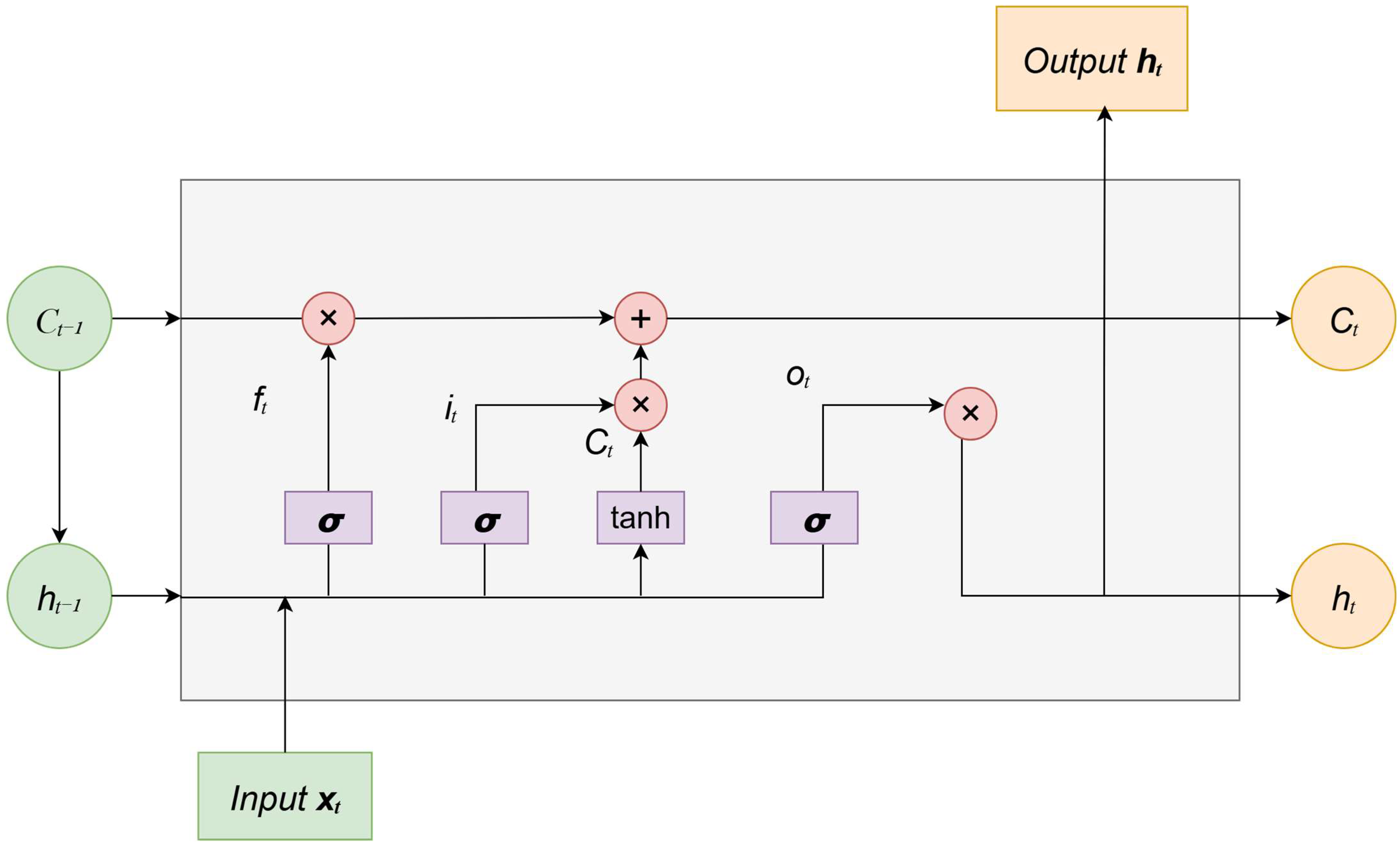
LSTM is a version of the Recurrent Neural Network (RNN) used to process sequence data and time series problems. Proposed by Hochreiter and Schmid Huber in 1997, it quickly became popular after the RNN solved the gradient descent problem. The LSTM network was created to address the problem traditional RNNs face in dealing with long-term dependencies. When a typical RNN processes long sequences, the gradient disappears or explodes progressively, making it difficult to capture long-term dependencies. LSTM addresses this problem by adding a gating mechanism. As shown in Figure 2, it primarily includes a memory unit, a forget gate $\left(f_t\right)$, an input gate ${(i}_t)$, and an output gate ${(o}_t)$. The input gate determines how much new information is added to the unit state, the forget gate controls whether it will be forgotten at any given time, and the output gate determines whether any information is output at any given time [35].

The cell state, which can be thought of as a container for storing information, progressively modifies and outputs information by controlling the processes of the input, forget, and output gates. Each cell state within a neural unit goes through the forget gate, the input gate, and the process of transferring information to the output gate. To process the current neural unit, the input gate duplicates the incoming data. The complete input consists of two components. The sigmoid activation function part specifies which input data categories are updated, i.e., discarded. The hyperbolic tangent function (tanh) was used to produce a new candidate value vector, which was then added to the current cell state. The mathematical procedure is as follows [37]:

$$i_t=\sigma \left(W_i\left[x_t{\cdot h}_{t-1}\right]+b_i\right)$$

(1)

$$c_t=\phi \left(W_c\left[x_t{\cdot h}_{t-1}\right]+b_c\right)$$

(2)

The forget gate is used to establish what information in the current state should be discarded, while the LSTM algorithm acquires the ability to instruct the network to retain information [37].

$$f_t=\sigma \left(W_f\left[x_t.h_{t-1}\right]+b_f\right)$$

(3)

The output gate is primarily responsible for controlling the output information of the current hidden state [37].

$$h_t=o_t⨂\phi \left(c_t\right)$$

(4)

$$c_t=i_t ⨂ c_t+f_t ⨂ c_{t-1}$$

(5)

$$o_t=\sigma \left(W_o\left[x_t.h_{t-1}\right]+b_o\right)$$

(6)

In the equation, $x_t$ represents the input and $h_t$ denotes the output of the network at $t$ time. Meanwhile, $c_t$ represents the newly formed candidate value vectors for the tanh component at $t$ time. The $f_t$, $i_t$, and $o_t$ elements refer to the forget, input, and output gates, respectively. The $W_f$, $W_i$, $W_o$, and $W_c$ matrices correspond to the weights associated with the forget, input, output, and memory cells. Furthermore, $b_f$, $b_i$, $b_o$ and $b_c$ denote the bias vectors associated with the forget, input, output, and memory cells, respectively. Function $\sigma$ represents the sigmoid function, while $\phi$ represents the tanh function. To acquire optimal parameters that improve the LSTM model performance, errors and gradients are calculated using the time backpropagation technique. Backpropagation in LSTM networks involves calculating gradients over time, modifying network parameters, and controlling the propagation of information through cell and gate states. The ability of LSTM to capture long-term dependencies in sequential data makes it highly suitable for time series prediction [37].

2.3.2. Convolutional Neural Network–Long Short-Term Memory (CNN–LSTM)

The CNN–LSTM hybrid architecture combines the strengths of convolutional and recurrent neural networks to enhance the modeling of complex temporal sequences. In this architecture, the CNN component acts as a feature extractor, capturing local temporal dependencies and patterns within the input data through convolution and pooling operations. These extracted features are then passed to the LSTM layers, which are capable of learning and preserving long-term dependencies and temporal dynamics over time [38].

This combination allows the model to effectively handle both spatial or local feature extraction and sequential learning, making it well-suited for time series forecasting tasks. In particular, the CNN–LSTM model has demonstrated strong performance in capturing short-term fluctuations while maintaining sensitivity to long-term trends, which is crucial for meteorological and environmental prediction.

In this study, the CNN–LSTM hybrid model was implemented to predict meteorological variables associated with Santa Ana wind conditions in the Guadalupe Basin. The convolutional layers were used to extract relevant temporal patterns from the input sequences, while the LSTM layers modeled their sequential evolution, enhancing the predictive capability of the system under complex and nonlinear atmospheric dynamics.

2.3.3. Bidirectional Long Short-Term Memory (BiLSTM)

Bidirectional Long Short-Term Memory (BiLSTM) networks are a specialized type of recurrent neural network (RNN) that incorporate two cell-state propagation paths: one moving forward (from past to future) and another moving backward (from future to past). This bidirectional architecture enables BiLSTM to capture both past and future temporal dependencies, allowing the model to learn contextual relationships in both directions. By processing the sequence in two opposite temporal orders, BiLSTM networks enhance the representation of temporal dynamics, particularly when future context contributes valuable information to the current prediction. This dual flow of information improves the model’s ability to understand complex temporal patterns in time series forecasting and sequence classification tasks [39].

The Bidirectional Long Short-Term Memory with Attention (BiLSTM-Attention) architecture enhances the learning capacity of recurrent neural networks by integrating a self-attention mechanism. While the BiLSTM component captures temporal dependencies in both forward and backward directions, the attention layer allows the model to assign different weights to each time step in the input sequence. This mechanism enables the network to focus on the most relevant temporal features that contribute to the target prediction, improving interpretability and predictive performance.

The attention mechanism computes a context vector as a weighted sum of the hidden states, where the weights are learned through a soft alignment process. This allows the model to dynamically prioritize the most informative portions of the sequence during training, resulting in better generalization, especially in time series with irregular or long-term dependencies.

2.4. Training and Validation Procedure

All deep learning models were trained using daily meteorological time series from MERRA-2 (1980–2020), preprocessed and standardized to the range [0, 1] through Min–Max normalization. The input sequences consisted of 90 consecutive days (look-back window) used to predict the next day’s values for the six variables under study: wind speed, wind direction (represented by its sine and cosine components), temperature, relative humidity, and atmospheric pressure.

The data were split chronologically into training (70%), validation (15%), and testing (15%) sets to preserve the temporal structure and prevent data leakage. The validation subset was used to monitor overfitting and tune hyperparameters, while the test subset was reserved for independent evaluation.

All models were trained using the Adam optimizer with a learning rate of 0.001, the Huber loss function, and Mean Absolute Error (MAE) as an additional evaluation metric. Training was performed for up to 100 epochs, with an early stopping criterion monitoring the validation loss and restore_best_weights = True. Patience values of 8–10 epochs were used, depending on the model complexity. The batch size was fixed to 32 across all experiments to balance learning stability and computational efficiency.

• LSTM baseline model
  The baseline network consisted of two stacked LSTM layers with 64 and 32 hidden units, respectively, followed by a Dense (16, ReLU) layer and a final linear output layer with six neurons (one per variable). A Dropout rate of 0.2 was applied to recurrent layers to mitigate overfitting. This configuration provided the reference benchmark for comparison with hybrid and fine-tuned models.
• CNN–LSTM hybrid model
  The CNN–LSTM model introduced a Conv1D layer (64 filters, kernel size = 3, ReLU activation) to extract short-term temporal patterns from the input sequences, followed by a MaxPooling1D layer (pool size = 2) to reduce noise and dimensionality. The convolved output was passed to an LSTM layer with 64 units, followed by Dropout (0.3) and a Dense (32, ReLU) layer before the output.
  This hybrid architecture allowed the network to capture both local temporal dependencies (via convolution) and longer-term trends (via recurrence).
• BiLSTM with Attention
  This architecture combined two Bidirectional LSTM layers (64 and 32 units) with an attention mechanism to enhance the model’s ability to focus on the most relevant time steps for prediction.
  Attention was implemented through learned query, key, and value projections (Dense (64)), followed by a scaled dot-product attention layer. The attention output was concatenated with the original BiLSTM output, forming a residual connection that improved gradient flow and contextual learning. A Dropout rate of 0.2 was applied to recurrent and attention layers.
  This model achieved improved learning of complex temporal dependencies, particularly in wind-related variables.
• Conv1D + BiLSTM + Attention hybrid model
  A more advanced hybrid architecture was tested to combine the local feature extraction of CNNs with the bidirectional temporal context of LSTMs and the adaptive focus of the attention mechanism.
  The model began with a Conv1D layer (64 filters, kernel size = 3, ReLU), followed by BatchNormalization and Dropout (0.2). The extracted features were processed through a Bidirectional LSTM layer (64 units, return_sequences = True), and an attention block composed of query, key, and value projections (Dense(64)) with scaled attention.
  The attention output was linearly transformed (Dense(128)) and added residually to the BiLSTM output before normalization (LayerNormalization).
  A second Bidirectional LSTM layer (32 units) summarized the contextual information before a Dense(n_features) output layer.
  This model showed improved generalization and robustness across all variables, especially under high-variability wind conditions.
• Fine-tuned LSTM model
  The baseline LSTM was further refined through a two-phase training strategy.
  In the first phase, the model was trained normally to convergence.
  In the second phase, sample weights were introduced to emphasize cases associated with local Santa Ana–like wind conditions, identified as days with wind speeds > 4.5 m/s and wind direction within 0–90° (first quadrant).
  Samples meeting this criterion were assigned three times higher weights (×3) to improve the network’s sensitivity to extreme and directional wind patterns.
  This fine-tuning phase enhanced the model’s predictive skill for rare or extreme conditions while maintaining global performance stability.

Hyperparameter Search and Model Selection

An automated hyperparameter search based on random sampling was performed to explore key architectural and optimization parameters (number of LSTM units and layers, convolutional kernel sizes for Conv1D, dropout rates, L1/L2 regularization, activation functions, batch size and learning rate). The search was implemented using a random search strategy (Keras Tuner RandomSearch was used for the experiments reported here), which balanced exploration of the hyperparameter space and computational cost. The following ranges/options were explored empirically during tuning:

• Input (look-back) windows: 60, 90, 120, 150, and 180 days (90 days produced the best overall trade-off between predictive skill and model complexity for most variables);
• Forecast horizons: 1, 3, and 15 days ahead (1-day horizon used for the main experiments reported);
• LSTM units (per layer): typically, 32–256 (final configurations reported in the text indicate 64 or 100 units depending on model);
• Number of recurrent layers: 1–2 (single layer for baseline LSTM; stacked/bidirectional variants for hybrid models);
• Conv1D filters: 16–128 with kernel sizes tested between 3 and 11 timesteps;
• Dropout rates: 0.01–0.3 (0.01 used for some LSTM layers; 0.2–0.3 for hybrid models to counteract overfitting);
• Regularization: L1 and L2 penalties tried in the order of 0.01 for selected Dense layers;
• Activation functions: ReLU and ELU evaluated for Dense layers;
• Batch sizes: 32, 72, and 128 tested (final reported runs used 32 for hybrid models and 128 for some baseline LSTM experiments depending on resource constraints);
• Optimizers and learning rates: Adam with learning rates in the range 1 × 10⁻⁴–1 × 10⁻³ (learning_rate = 1 × 10⁻³ used for the final models).

Early stopping and dropout regularization were systematically applied to mitigate overfitting.

The training process logged the evolution of loss and validation metrics at each epoch, and convergence was visually inspected using learning curves.

The final models reported correspond to the configurations that minimized validation loss and achieved the best trade-off between accuracy and generalization.

Table 1. Summary of the main configurations and hyperparameters of the deep learning architectures evaluated.

Model	Architecture	Key Layers/Units	Dropout	Attention	Optimizer	Loss Function	Batch Size	Epochs	Early Stopping	Look-Back Window
LSTM (baseline)	2 × LSTM (64,32) + Dense (16, ReLU) + Output (6)	64–32 LSTM	0.2	No	Adam (lr = 0.001)	Huber	32	100	Patience = 10	90
CNN–LSTM	Conv1D (64, k = 3) + MaxPool + LSTM (64) + Dense (32, ReLU)	64 filters	0.3	No	Adam (lr = 0.001)	Huber	32	100	Patience = 8	90
BiLSTM + Attention	2 × BiLSTM (64,32) + Attention + Dense (6)	64–32 BiLSTM	0.2	Yes	Adam (lr = 0.001)	Huber	32	100	Patience = 8	90
Conv1D + BiLSTM + Attention	Conv1D (64, kernel = 3) Conv1D (64, k = 3) + BiLSTM (64,32) + Attention + Dense (6)	64–32 BiLSTM	0.2	Yes	Adam (lr = 0.001)	Huber	32	100	Patience = 8	90
Fine-tuned LSTM	LSTM baseline + weighted training (×3 for SAW)	64–32 LSTM	0.2	No	Adam (lr = 0.001)	Weighted Huber	32	30 + 10	Patience = 8	90

summarizes the hyperparameter configurations and architectural details of the deep learning models tested. These configurations were derived from a combination of empirical tuning and random search using Keras Tuner. The selected settings represent the best-performing variants in terms of validation loss and generalization performance.

2.5. Model Evaluation Metrics

The following performance metrics were used to evaluate the predictive accuracy of the deep learning models. Standard statistical indicators were applied to the continuous variables (wind speed, temperature, relative humidity, and pressure), while specialized angular metrics were used for wind direction.

2.5.1. Standard Metrics

The Root Mean Square Error (RMSE), Mean Absolute Error (MAE), and Coefficient of Determination (R²) were computed as follows [14]:

$$RMSE=\sqrt{{\displaystyle \frac{1}{n}}\sum _{i=1}^n{\left(y_i-{\widehat{y}}_i\right)}^2}$$

(7)

$$R^2=\sum _{i=1}^n{\left({\widehat{y}}_i-{\overline{y}}_i\right)}^2/\sum _{i=1}^n{\left(y_i-{\overline{y}}_i\right)}^2$$

(8)

$$MAE={\displaystyle \frac{1}{n}}\sum _{i=1}^n\left|y_i-{\widehat{y}}_i\right|$$

(9)

where $n$ is the number of data points, $y_i$ is the observed value, ${ \widehat{y}}_i$ the predicted value, and ${\overline{y}}_i$ is the mean of the observed data.

2.5.2. Angular Metrics for Wind Direction

Since wind direction is a circular variable ranging from 0° to 360°, conventional metrics are inadequate because they do not account for angular discontinuities (e.g., 359° and 1° are only 2° apart). To handle this, wind direction was first decomposed into its trigonometric components—sine and cosine—prior to model training:

$${wd}_{sin}=\sin \left(\theta \right)$$

(10)

$${wd}_{cos}=\cos \left(\theta \right)$$

(11)

After prediction, the direction was reconstructed using the inverse tangent function:

$$\widehat{\theta }=\mathrm{atan}2\left({\widehat{wd}}_{sin}{\widehat{wd}}_{cos}\right)\times {\displaystyle \frac{180}{\pi }}$$

(12)

The model’s angular accuracy was then quantified using the Mean Absolute Error (MAE) and Root Mean Square Error (RMSE) for angular data:

$${MAE}_{ang}={\displaystyle \frac{1}{n}}\sum _{i=1}^n\left|\mathsf{\Delta }{\theta }_i\right|$$

(13)

$${RMSE}_{ang}=\sqrt{{\displaystyle \frac{1}{n}}\sum _{i=1}^n{\left(\mathsf{\Delta }{\theta }_I\right)}^2}$$

(14)

where $\mathsf{\Delta }{\theta }_I=min\left(\left|{\theta }_i-{\widehat{\theta }}_i\right|, 360°- \left|{\theta }_i-{\widehat{\theta }}_i\right|\right)$ ensures that angular differences wrap around the 360° circle correctly.

2.6. Identification of Santa Ana Wind Conditions

In previous research [7,36], a filter was developed to identify days potentially associated with Santa Ana wind (SAW) conditions. This filter was derived from a review of existing classification methodologies and adapted to the requirements of quantitative time series modeling. The operational criterion defines SAW-like conditions as days with wind speed ≥ 4.5 m/s and wind direction within the first quadrant (0–90°). This threshold-based approach enables the construction of consistent numerical series suitable for fractal and multifractal analyses while maintaining coherence with local SAW characteristics described in the literature.

It is important to note that Santa Ana winds are large-scale synoptic phenomena primarily driven by pressure gradients between the Great Basin and the Pacific coast. Therefore, the objective of this study is not to forecast SAW events directly, but rather to model and analyze the temporal dynamics of the local meteorological variables that typically accompany such conditions—namely, wind speed, wind direction, temperature, relative humidity, and atmospheric pressure.

Accordingly, the adopted filter should be interpreted as a local proxy that identifies periods exhibiting meteorological signatures consistent with SAW conditions at the basin scale. This approach provides a practical framework for evaluating model performance under extreme or anomalous atmospheric regimes, consistent with previous operational methodologies applied in Southern California and northern Baja California [3,12,40,41].

2.7. Fractal Theory

Mandelbrot described a fractal as a set for which its Hausdorff dimension is greater than its topological dimension. He also defined the fractal dimension as a non-integer value, which allows describing fractal geometry, as well as the heterogeneity of irregular figures, allowing the capture of information lost when using traditional geometric representations. The fractal dimension is related to the Hurst exponent through the following equation developed by Voss [42]:

$$2\mathrm{H}+1=5-2\mathrm{D}$$

(15)

Solving the above equation, a direct relationship is obtained between the fractal dimension $\left(\mathrm{D}\right)$ and the Hurst exponent $\left(\mathrm{H}\right)$. Therefore,

$$\mathrm{D}=2-\mathrm{H}$$

(16)

The fractal dimension D and the Hurst exponent $\mathrm{H}$ obtained from the analyzed series allow us to determine the persistence or anti-persistence characteristics.

2.8. Methodology

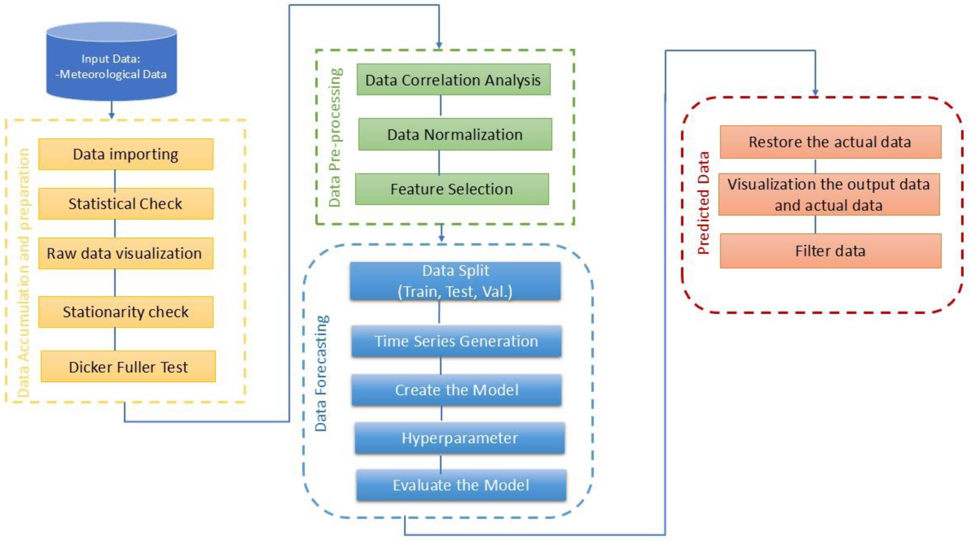
Figure 3 shows the detailed methodology used, divided into data collection and preparation if required, analysis of the stationarity of the time series, verification of correlations between variables, the prediction model, and the filter applied at the end of the forecast.

2.9. Computational Environment

The model was implemented in Python 3.10.9 using TensorFlow 2.10 and Keras 2.10 on an Acer laptop (Acer Inc., Taiwan, China) with an Intel® Core™ i5-7200U CPU @ 2.50 GHz, 8 GB RAM, and an NVIDIA GeForce MX130 GPU running Windows 10 Intel^® Core™ i5-7200U CPU @ 2.50 GHz.

3. Results and Discussion

3.1. Data Series and Trend Analysis

The meteorological dataset used for model development consists exclusively of MERRA-2 reanalysis variables—wind speed, wind direction, temperature, relative humidity, and air pressure—covering the period 1980–2020 at the Guadalupe Basin. In addition, in situ measurements from the Agua Caliente meteorological station (elevation 400 m; 1 January 1969–31 October 2012) provide daily temperature and precipitation records. These observational data are used solely to validate and compare statistical properties with the reanalysis data; they are not included in model training, testing, or prediction.

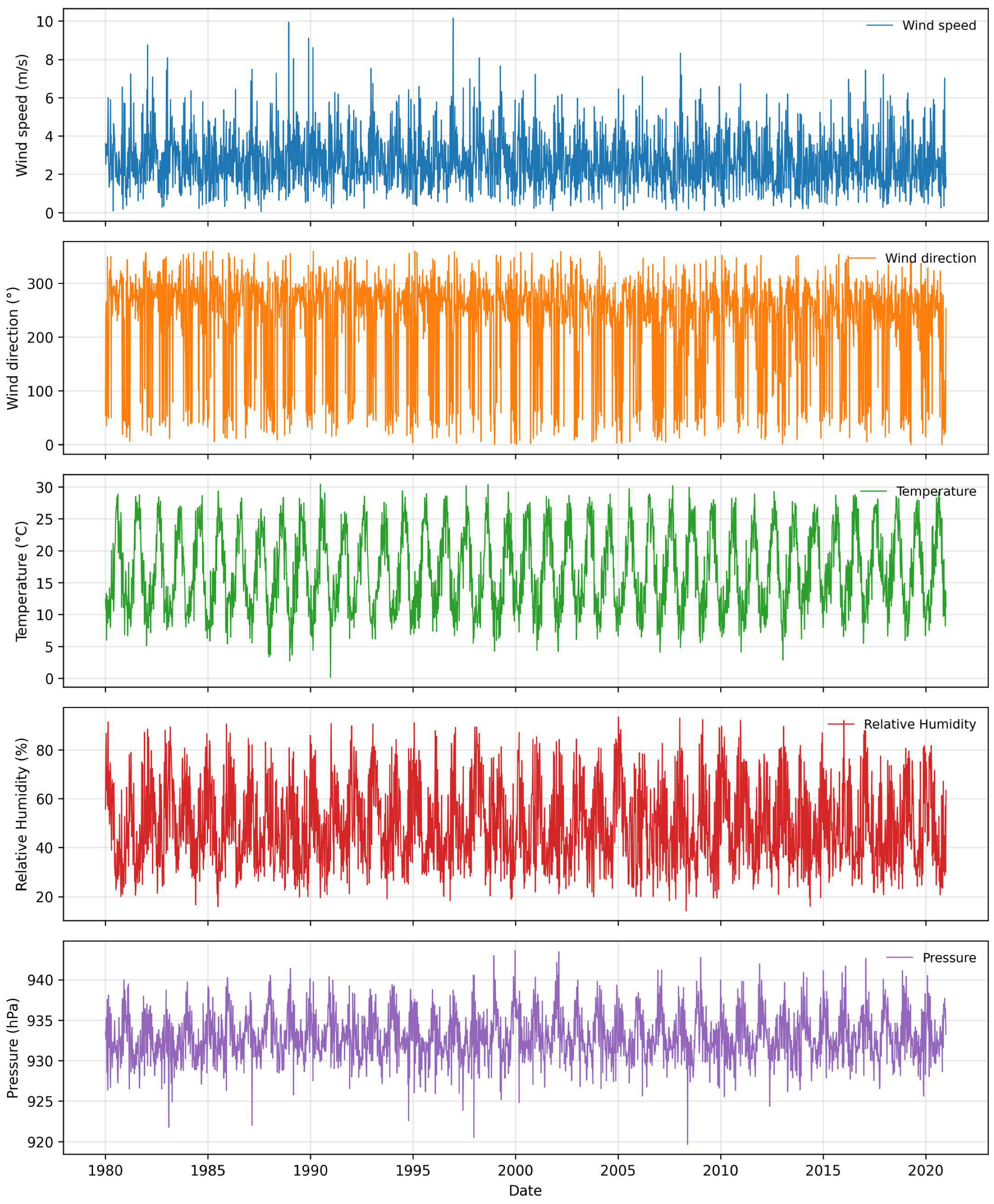
Figure 4 presents the daily MERRA-2 records of wind speed, wind direction, temperature, relative humidity, and air pressure.

To provide a comprehensive overview of the meteorological conditions at the Guadalupe Basin, the daily MERRA-2 data were subjected to a detailed statistical analysis. This analysis characterizes the central tendency, dispersion, and distribution of each variable, offering insights into their variability and typical behavior over the 1980–2020 period. The results include measures such as mean, median, standard deviation, variance, skewness, kurtosis, and selected percentiles, which collectively describe both the average conditions and the occurrence of extreme events.

Table 2. Descriptive statistics of meteorological variables (1980–2020) from the MERRA-2 grid cell corresponding to the Agua Caliente station location.

	Wind Speed (m/s)	Wind Direction (°)	Temperature (°C)	Relative Humidity (%)	Pressure (hPa)
count	14,976	14,976	14,976	14,976	14,976
mean	2.70	225.46	16.81	49.34	932.85
std	1.42	94.58	6.24	16.88	2.95
min	0.02	0.08	0.11	12.12	913.49
25%	1.71	206.48	11.64	36	930.92
50%	2.51	261.49	16.11	46.43	932.6
75%	3.44	287.07	22.2	61.48	934.68
max	10.63	359.99	33.24	95.38	945.04
var	2.01	8944.79	38.99	285.00	8.73
skew	0.92	−1.09	0.17	0.45	0.18
kurt	1.34	−0.16	−1.04	−0.67	0.76

summarizes these descriptive statistics for all variables, serving as a foundation for subsequent interpretation of climatological patterns and model performance.

Wind speed shows a mean of 2.70 m/s, indicating a generally calm to light breeze regime according to the Beaufort scale [43]. The standard deviation of 1.42 m/s reflects moderate variability within the historical record. Percentile values fluctuate around the mean, suggesting relatively stable conditions. The maximum observed wind speed of 10.63 m/s corresponds to occasional gusts likely associated with synoptic events, while minimum values near zero indicate calm days.

Wind direction exhibits a mean of 225.46°, indicating a predominant southwest flow. The large standard deviation (94.58°) and variance (8944.79) reveal high directional variability, consistent with the influence of topographic constraints and seasonal wind patterns in the Guadalupe Basin. Kurtosis (−0.16) suggests a nearly normal distribution with slightly shorter tails, while skewness (−1.08) indicates a slight bias toward westerly directions.

Temperature averages 16.81 °C with a standard deviation of 6.24 °C and values ranging from 0.11 °C to 33.24 °C. The 25th and 75th percentiles (11.64–22.2 °C) indicate that most days fall within moderate thermal conditions, while extremes reflect seasonal variability. Skewness (0.17) and kurtosis (−1.04) suggest a fairly symmetric, slightly flattened distribution with low frequency of extreme temperature events. These patterns are consistent with the basin’s transitional climate between coastal and continental influences.

Relative humidity has a mean of 48.59% with a standard deviation of 16.88%. The distribution exhibits slight positive skewness (0.45) and a kurtosis of −0.67, indicating a relatively flat distribution with occasional high humidity episodes, likely corresponding to periods of increased moisture influx from coastal systems.

Air pressure shows the lowest variability, with a mean of 932.94 hPa and a standard deviation of 2.95 hPa. The kurtosis (0.76) and small positive skewness (0.18) suggest a near-normal distribution with slightly heavier tails, reflecting occasional synoptic-scale pressure variations.

Overall, wind direction and relative humidity display high variability, influenced by seasonal and topographic effects, while temperature and pressure remain comparatively stable. These patterns provide essential climatological context for evaluating the predictive performance of the model.

The consistency between MERRA-2 reanalysis temperature and in situ station measurements supports the use of MERRA-2 data for model development. The daily mean temperature from MERRA-2 (16.81 °C) is comparable to the station observations (18.08 °C), while standard deviations (6.24 °C vs. 5.75 °C) and overall ranges indicate similar variability. Although MERRA-2 may slightly smooth extreme values due to its spatial and temporal resolution, these statistics demonstrate that the reanalysis captures the main climatological features at the station location, providing a reliable basis for predictive modeling.

The Augmented Dickey–Fuller (ADF) test confirms the stationarity of all MERRA-2 variables.

Table 3. Augmented Dickey–Fuller test results for MERRA-2 time series.

	Wind Speed	Wind Direction	Temperature	Relative Humidity	Pressure
ADF Statistic	−15.4704	−11.3235	−7.7615	−12.0521	−11.4776
p-value	2.63 × 10−28	1.16 × 10−20	9.43 × 10−12	2.58 × 10−22	5.09 × 10−21
Critical values
1%	−3.4308	−3.4308	−3.4308	−3.4308	−3.4308
5%	−2.8617	−2.8617	−2.8617	−2.8617	−2.8617
10%	−2.5669	−2.5669	−2.5669	−2.5669	−2.5669
lag	36	39	37	31	34
nobs *	14,939	14,936	14,938	14,944	14,941

* nobs = The number of observations used for the ADF regression and calculation of the critical values.

shows that ADF statistics exceed MacKinnon critical values at 1%, 5%, and 10% significance levels, with p-values below 0.05, confirming stationarity in all series.

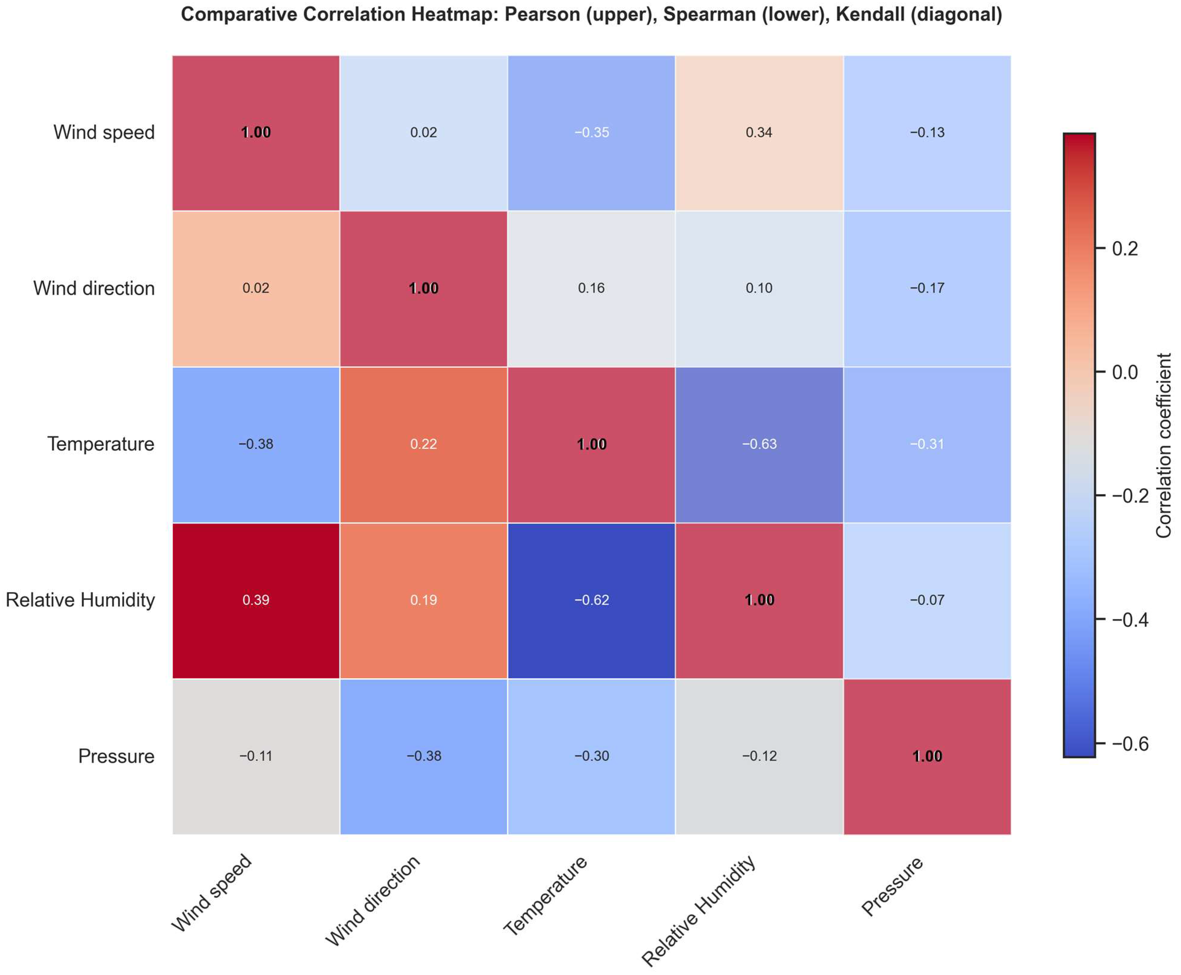
Figure 5 presents a comparative correlation heatmap among the five MERRA-2 variables using Pearson (upper triangle), Spearman (lower triangle), and Kendall (diagonal) coefficients. Temperature and relative humidity show a strong inverse correlation (r ≈ −0.63), wind speed and temperature a moderate negative correlation (r ≈ −0.35), and wind direction exhibits weak correlations with other variables (|r| < 0.25). The similarity between Pearson and rank-based correlations suggests that most relationships are monotonic but not strictly linear, supporting the inclusion of non-linear structures in the forecasting model.

3.2. Seasonal Characterization of Santa Ana Wind Conditions

To further understand the local meteorological dynamics influencing wind behavior in the Guadalupe Basin, the occurrence of Santa Ana wind (SAW) conditions was analyzed throughout the 1980–2020 period. Days meeting the criteria of wind speed ≥ 4.5 m s⁻¹ and wind direction within the first quadrant (0–90°) were classified as Santa Ana–like events, following the operational filter described in Section 2.6. A total of 373 such days were identified out of 14,976 daily records, representing approximately 2.5% of the dataset.

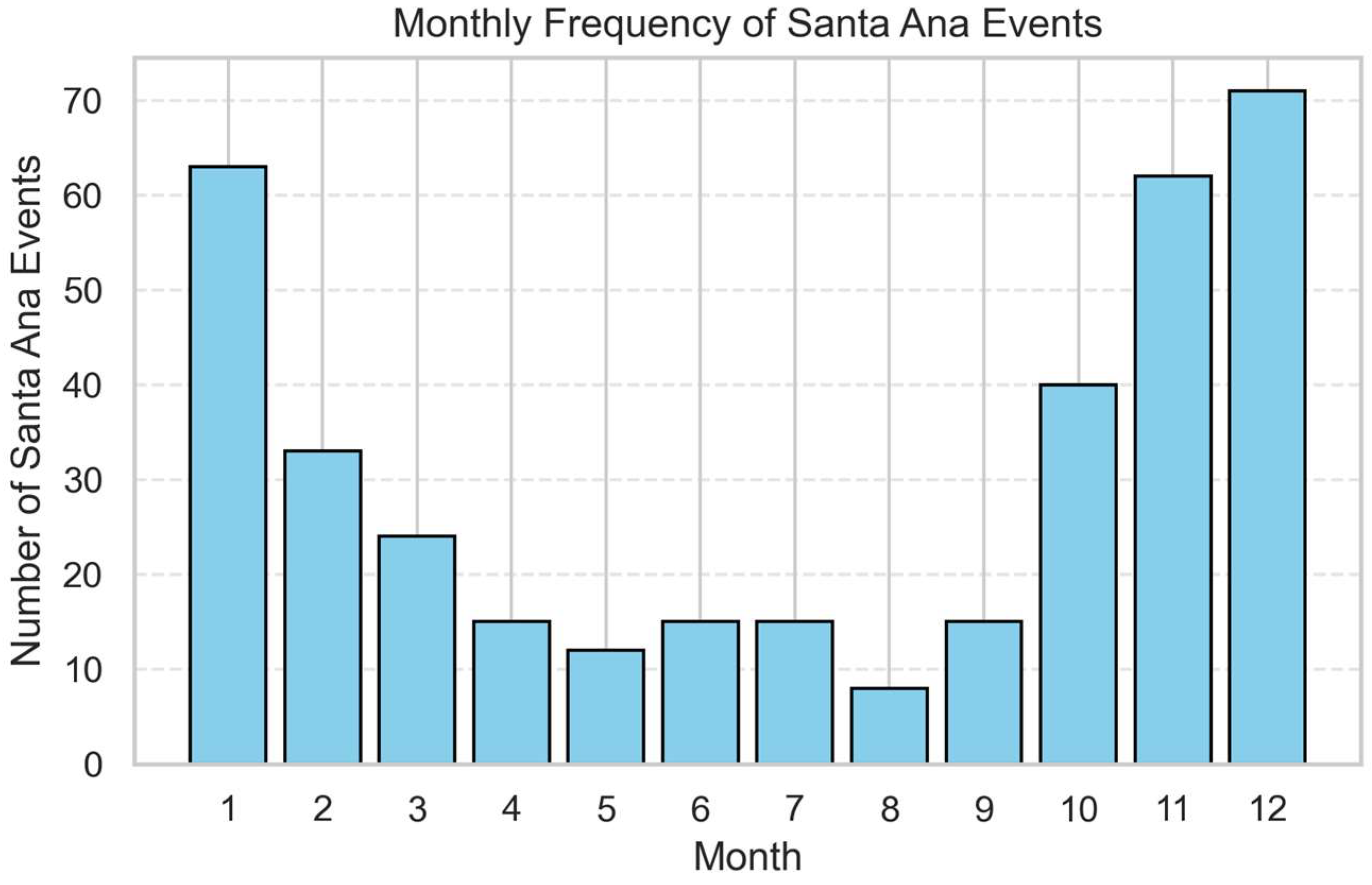
The analysis reveals a pronounced seasonal pattern in the occurrence of SAW conditions. Figure 6 shows that events are predominantly concentrated between October and February, corresponding to the cool season, with a marked peak in December and January. In contrast, events are nearly absent during the summer months, indicating a clear intra-annual periodicity consistent with the regional climatology of downslope, dry wind episodes.

The intra-annual distribution (Figure 7) further highlights this seasonal clustering. The highest frequencies occur during winter, with a sharp decline in spring and almost no events during the summer. Most Santa Ana occurrences appear as isolated, single-day episodes, while multi-day sequences are relatively rare, suggesting that SAW conditions in this basin manifest as short-lived but intense events rather than prolonged wind episodes.

Analysis of Figure 8 indicates that most Santa Ana events occur as isolated, single-day episodes. Only a small fraction of events extend over consecutive days, suggesting that Santa Ana winds in the dataset predominantly occur as short-lived phenomena rather than prolonged sequences.

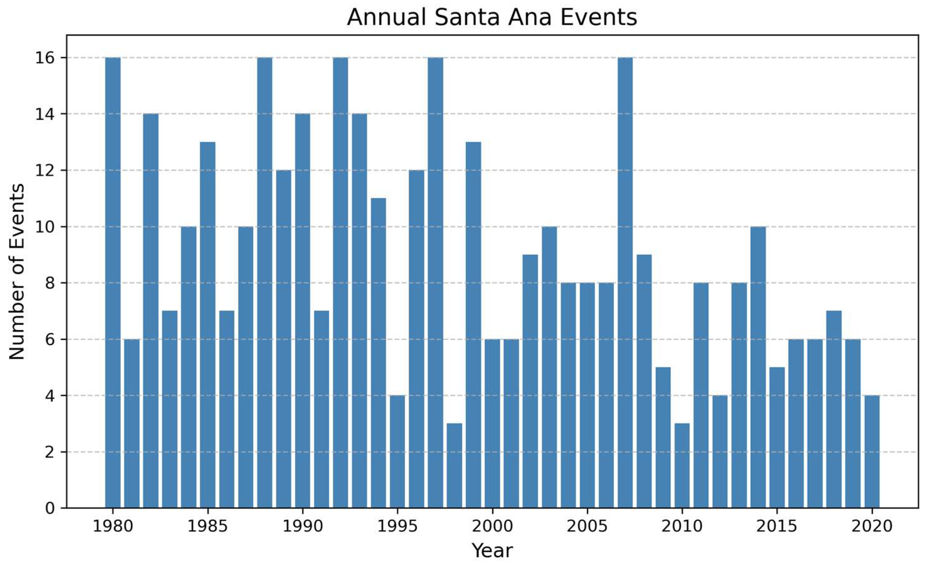
The interannual variability of Santa Ana events (Figure 8) indicates a non-monotonic temporal behavior with alternating phases of high and low activity. Over the 40-year record, the total number of annual events ranges from 3 to 16, with a long-term mean of 9.1 events yr⁻¹. Notable peaks were observed in 1980, 1988, 1992, 1997, and 2007, whereas years such as 1998 and 2010 registered only three events. These fluctuations reflect the episodic and irregular nature of Santa Ana wind dynamics at the regional scale. Although some peak and low years coincide with known ENSO phases, formal attribution would require cross-correlation with standardized ENSO indices (e.g., Niño 3.4), which is recommended for future work.

Overall, this analysis confirms that Santa Ana wind events in the Guadalupe Basin are episodic, highly seasonal, and short in duration, representing a small fraction of the total time series. This climatological context provides critical insight into the variability and rarity of high-wind conditions later examined in the modeling stage.

3.3. Model Performance and Evaluation

This section presents the results of the deep learning models and the corresponding discussion of their predictive performance across the main meteorological variables. The analysis focuses on the model’s capacity to reproduce the temporal variability and interdependence of wind speed, wind direction, temperature, relative humidity, and atmospheric pressure over the 1980–2020 period.

All models were trained and validated following the procedures described in Section 2, ensuring chronological consistency and preventing data leakage. The evaluation was conducted using standard and angular performance metrics, as well as comparative visualization of observed and predicted series.

The predictive performance of the proposed models was evaluated using the test dataset for each target variable.

Table 4. Performance comparison of predictive models for temperature estimation.

Model	RMSE	MAE	R2
Climatology (baseline)	6.143	5.192	−0.009
Persistence model	1.788	1.409	0.914
LSTM	1.571	1.251	0.934
Fine-tuned LSTM	1.517	1.212	0.939
CNN + LSTM	1.752	1.391	0.918
BiLSTM + Attention	1.488	1.186	0.941
Conv1D + BiLSTM + Attention	1.781	1.421	0.915

,

Table 5. Performance comparison of predictive models for wind speed estimation.

Model	RMSE	MAE	R2
Climatology (baseline)	1.375	1.088	−0.015
Persistence model	1.414	1.042	−0.073
LSTM	1.137	0.860	0.306
Fine-tuned LSTM	1.116	0.837	0.333
CNN + LSTM	1.155	0.875	0.284
BiLSTM + Attention	1.19	0.838	0.327
Conv1D + BiLSTM + Attention	1.135	0.864	0.308

,

Table 6. Performance comparison of predictive models for wind direction estimation.

Model	RMSE Angular	MAE Angular
Climatology (baseline)	71.68°	54.87°
Persistence model	58.31°	40.87°
LSTM	51.728°	34.375°
Fine-tuned LSTM	51.856°	34.383°
CNN + LSTM	53.164°	36.109°
BiLSTM + Attention	50.938°	34.089°
Conv1D + BiLSTM + Attention	52.510°	35.019°

,

Table 7. Performance comparison of predictive models for relative humidity estimation.

Model	RMSE	MAE	R2
Climatology (baseline)	17.139	14.344	−0.000
Persistence model	11.008	8.031	0.587
LSTM	8.381	6.337	0.757
Fine-tuned LSTM	8.444	6.401	0.756
CNN + LSTM	8.874	6.819	0.732
BiLSTM + Attention	8.379	6.285	0.761
Conv1D + BiLSTM + Attention	8.719	6.675	0.741

and

Table 8. Performance comparison of predictive models for pressure estimation.

Model	RMSE	MAE	R2
Climatology (baseline)	2.912	2.266	−0.004
Persistence model	2.109	1.556	0.473
LSTM	1.714	1.280	0.652
Fine-tuned LSTM	1.738	1.311	0.640
CNN + LSTM	2.062	1.580	0.497
BiLSTM + Attention	1.729	1.300	0.646
Conv1D + BiLSTM + Attention	1.922	1.464	0.563

summarize the results in terms of RMSE, MAE, and R² (and angular metrics for wind direction). Baseline models (climatology and persistence) were included for reference to quantify the improvement achieved through deep learning architectures.

3.3.1. Training and Convergence Analysis

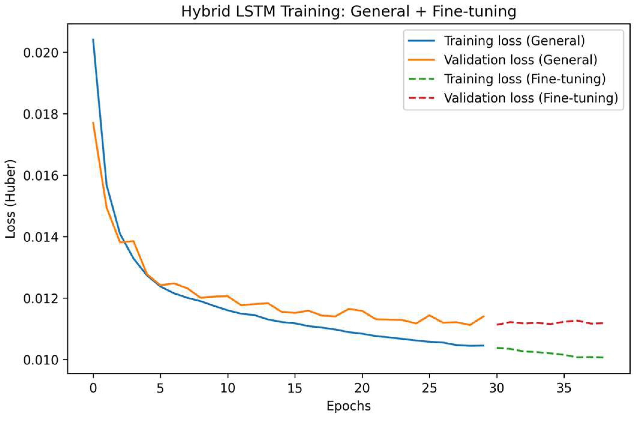
Figure 9 presents the training and validation loss curves of the hybrid fine-tuned LSTM model, developed through a two-stage learning strategy. In the general training phase (solid lines), both training and validation losses decreased smoothly and stabilized after approximately 25 epochs, indicating adequate convergence and the absence of overfitting.

The fine-tuning phase (dashed lines) further reduced the loss values, maintaining a consistent gap between training and validation curves. This behavior confirms that the model preserved its generalization ability while improving its responsiveness to high-intensity wind events emphasized through weighted training.

Overall, the stable convergence observed in both stages validates the robustness of the hybrid LSTM configuration and supports the credibility of the predictive performance reported in the following subsections.

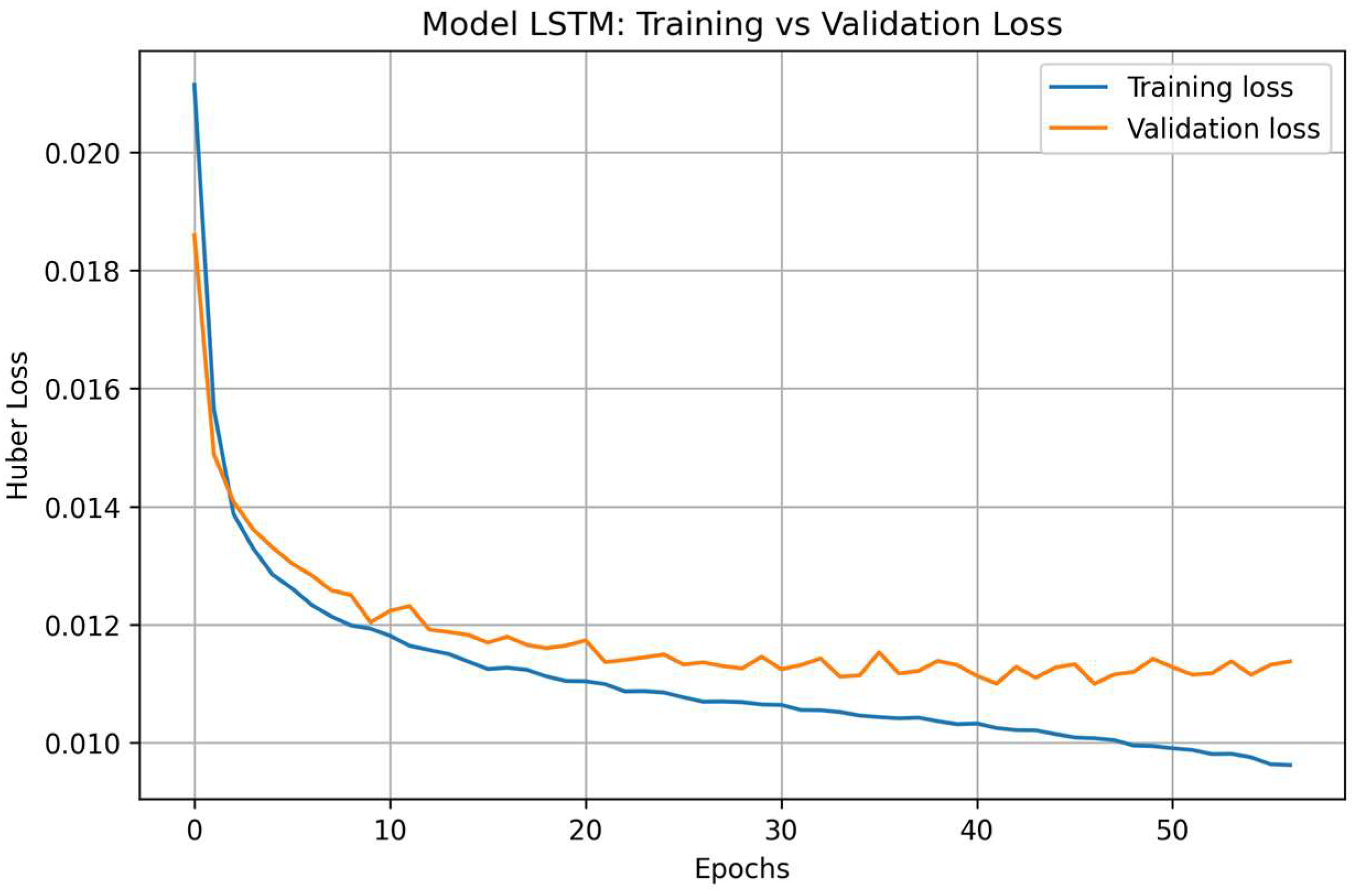
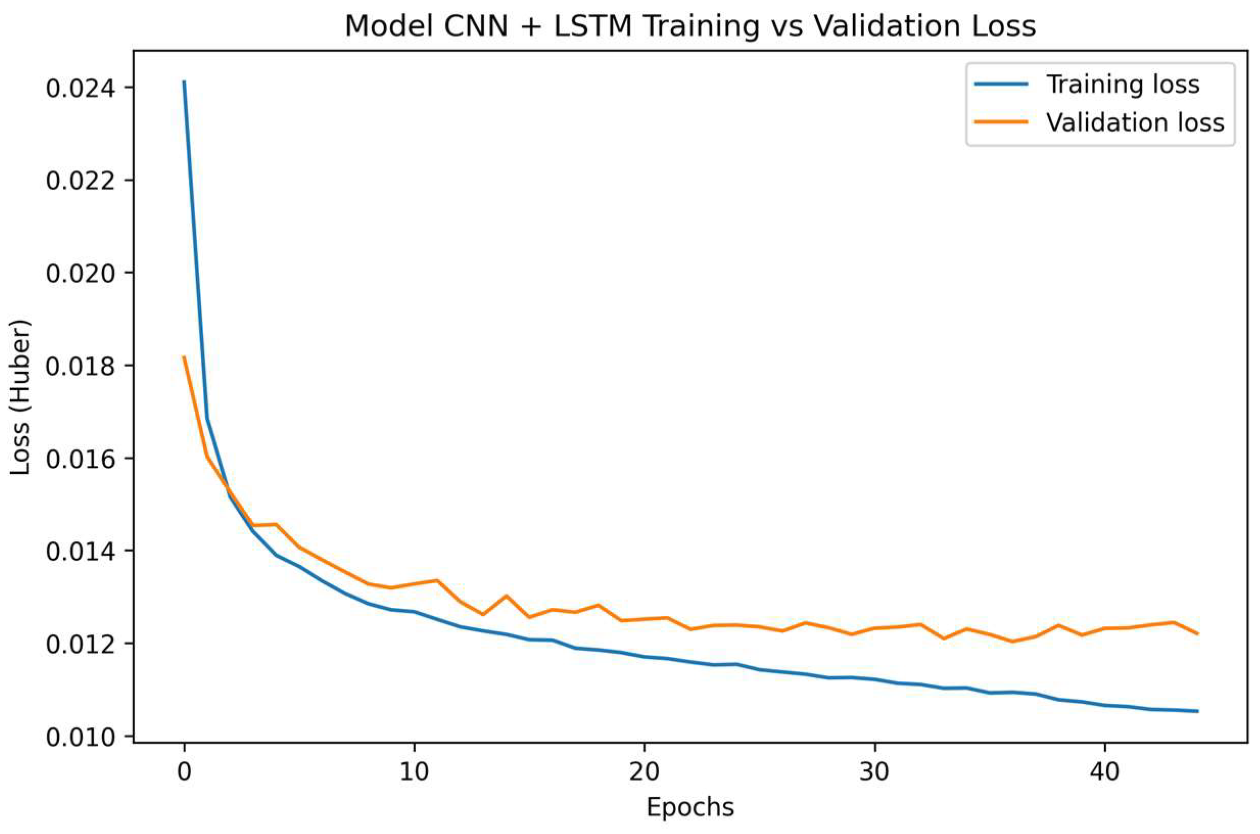
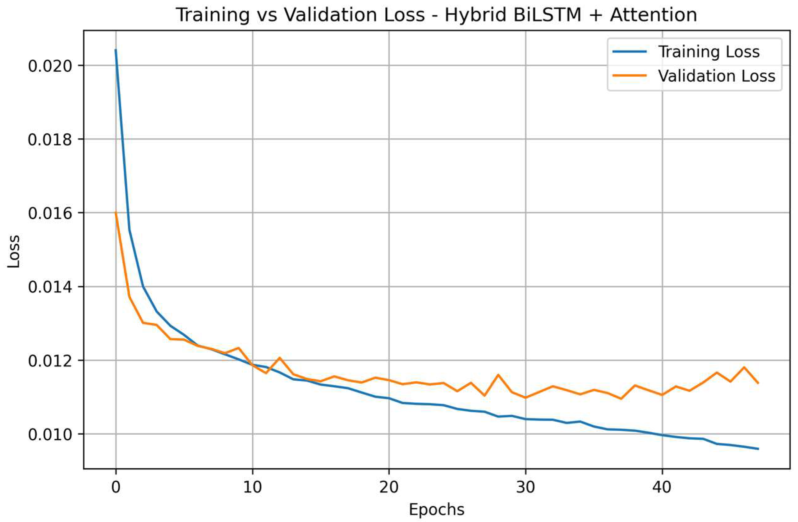
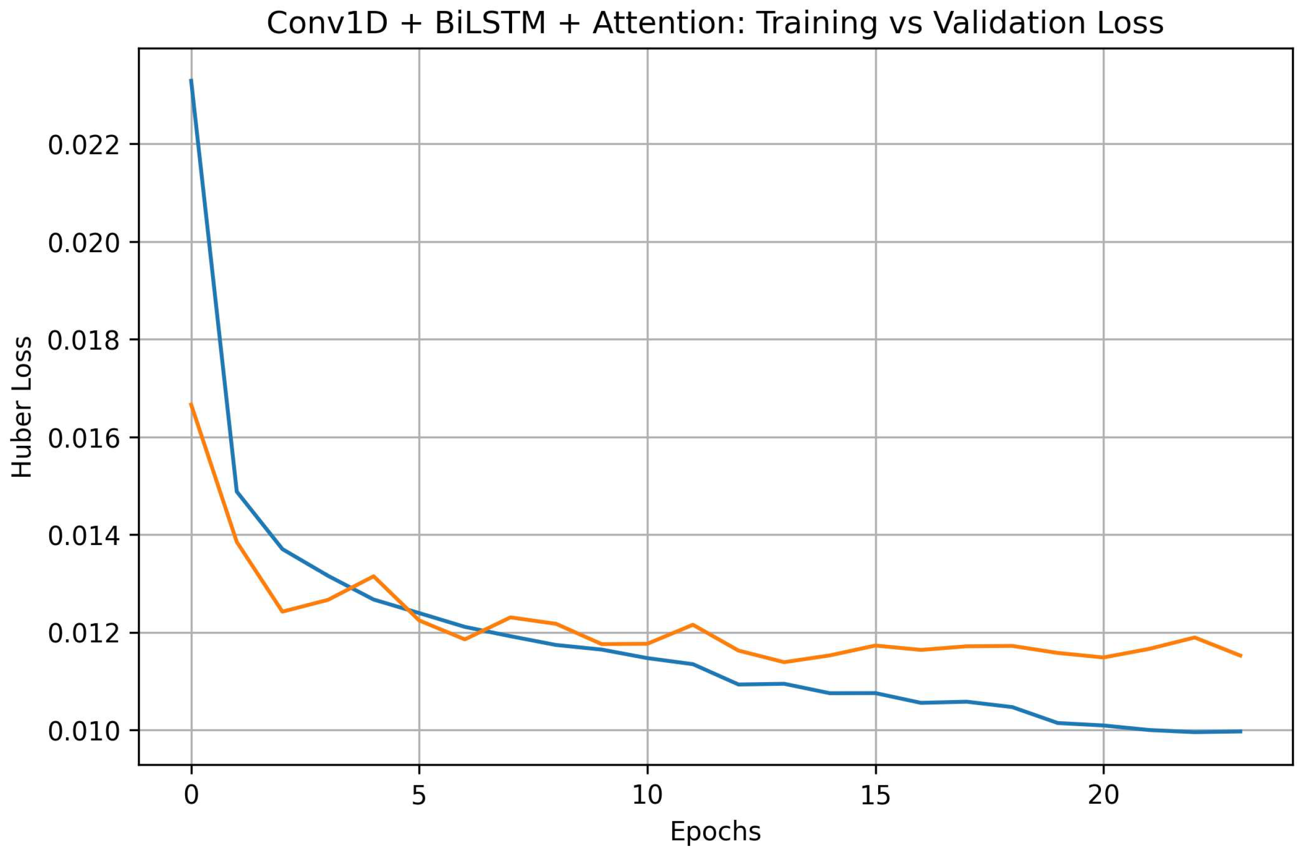
Additional learning curves for the remaining deep learning architectures (LSTM, CNN–LSTM, BiLSTM + Attention, and Conv1D + BiLSTM + Attention) are provided in Appendix A.1, showing similar convergence behavior and stable validation losses.

3.3.2. Temperature Forecasting

Two baseline models were established for comparison: (1) a climatology model, which predicts each day’s temperature as the long-term mean for the corresponding calendar day (computed from the training period), and (2) a persistence model, which assumes that the temperature of the next day is equal to that of the previous day. These baselines provide simple but informative benchmarks to evaluate the added predictive value of deep learning architectures.

Table 4 presents the performance metrics obtained for temperature prediction using different models, including the two baselines. The evaluation was performed on the test dataset to assess each model’s predictive accuracy and generalization capability. Overall, all deep learning models achieved consistent and robust performance, with determination coefficients (R²) exceeding 0.91 and low error magnitudes (RMSE < 1.8 °C).

Among them, the fine-tuned LSTM and BiLSTM + Attention configurations achieved slightly better accuracy, suggesting that attention mechanisms and adaptive weighting help capture subtle temporal dependencies and nonlinear patterns in temperature variability. In contrast, baseline models such as climatology and persistence exhibited considerably lower accuracy, confirming the relevance of data-driven architectures for temperature forecasting in the study area.

These results indicate that temperature is a relatively well-behaved and predictable variable in this region, likely due to its smoother temporal evolution compared to more stochastic variables such as wind speed or direction.

3.3.3. Wind Speed Forecasting

Two baseline models were also implemented for wind speed forecasting: (1) the climatology model, which predicts the long-term mean wind speed for each calendar day, and (2) the persistence model, which assumes that the wind speed remains constant from one day to the next. These baselines provide a reference for evaluating the skill of deep learning architectures in capturing temporal and nonlinear dynamics.

Table 5 summarizes the performance metrics for all models. All deep learning configurations substantially outperformed the baseline references, demonstrating their ability to capture short-term dependencies and nonlinear fluctuations in wind speed. The fine-tuned LSTM model achieved the best overall results, with the lowest RMSE (1.116 m·s⁻¹) and MAE (0.837 m·s⁻¹), and the highest R² (0.333), indicating improved generalization compared to the standard LSTM.

The CNN + LSTM and BiLSTM + Attention architectures also delivered competitive performance, confirming the robustness of hybrid and attention-based schemes in modeling temporal variability. The performance gains of the fine-tuned LSTM are attributed to the weighted training strategy, which emphasized high-intensity wind episodes associated with Santa Ana conditions. This weighting helped the model better represent the rare but dynamically significant extremes that are typically underrepresented in standard training schemes.

Nevertheless, the moderate R² values across models highlight the intrinsic complexity and stochasticity of wind dynamics at the local scale. Wind speed exhibits abrupt, high-frequency variability that poses a challenge for deterministic models. Despite these limitations, the results confirm the potential of deep learning models to improve upon baseline forecasts while capturing meaningful temporal structures in the data.

3.3.4. Wind Direction Forecasting (Angular Metrics)

To avoid the circular discontinuity between 0° and 360°, wind direction was decomposed into sine and cosine components during training and subsequently reconstructed into angular form for evaluation. The angular Mean Absolute Error (MAE) and Root Mean Square Error (RMSE) were used as evaluation metrics, defined over the minimal angular difference between predicted and observed directions. This formulation provides a consistent and physically meaningful measure of directional accuracy, independent of quadrant boundaries.

Table 6 presents the angular evaluation metrics for all models. Deep learning architectures substantially outperformed the climatology and persistence baselines, confirming their enhanced capacity to reproduce the temporal and directional variability of the wind field. Among the tested configurations, the BiLSTM + Attention model achieved the lowest angular errors (RMSE = 50.94°, MAE = 34.09°), slightly surpassing the fine-tuned LSTM and CNN–LSTM architectures. These results underscore the benefits of combining bidirectional memory with attention mechanisms, which allow the network to integrate past and future contextual information while dynamically weighting the most relevant time steps for prediction.

The relatively small differences among deep learning models suggest that the learned directional representations are robust and consistent across architectures, even under complex local wind regimes. However, attention-based models showed a slight edge in angular precision, highlighting their effectiveness in capturing nonlinear transitions in the sine–cosine space that represent directional shifts.

Although the models achieved substantial improvement over the climatology and persistence baselines, the angular errors (MAE ≈ 34°, RMSE ≈ 51°) are reasonable given the daily temporal resolution, the multivariate formulation, and the limited set of predictors. Reported angular errors for specialized or hourly wind direction models typically range between 25° and 40°, indicating that the present results are within an acceptable range. The complex topography of the Guadalupe Basin and the abrupt flow reversals associated with Santa Ana events further contribute to directional variability. Thus, despite inherent challenges in modeling circular variables, the proposed approach effectively reproduces the main directional patterns and transitions of the local wind regime.

3.3.5. Relative Humidity Forecasting

Table 7 summarizes the performance of all models in predicting relative humidity. All deep learning architectures markedly outperformed both climatology and persistence baselines, achieving R² values above 0.73. The BiLSTM + Attention model obtained the lowest errors (RMSE = 8.38, MAE = 6.29), followed closely by the standard and fine-tuned LSTM models.

These results indicate that recurrent architectures efficiently capture the temporal dynamics of humidity, which typically exhibits smoother variations and stronger autocorrelation than wind-related variables. The relatively small differences among models suggest that the added complexity of hybrid or attention mechanisms yields only marginal gains, as the variable’s lower short-term variability reduces the need for selective temporal weighting.

Overall, all models achieved consistent and stable predictions of daily relative humidity, confirming that LSTM-based models are well-suited for forecasting slowly varying meteorological variables within a multivariate framework.

3.3.6. Atmospheric Pressure Forecasting

Table 8 presents the performance metrics for atmospheric pressure prediction. All deep learning models significantly outperformed the climatology and persistence baselines, which exhibited R² values close to zero and moderate errors. Among the tested architectures, the LSTM achieved the best overall performance (RMSE = 1.71, MAE = 1.28, R² = 0.65), followed closely by the fine-tuned LSTM and BiLSTM + Attention models.

The CNN-based configurations yielded slightly higher errors, suggesting that convolutional feature extraction contributed less to capturing low-frequency pressure dynamics. These results indicate that pressure variations in the study area are largely governed by smooth, large-scale patterns, which can be efficiently represented by recurrent architectures without the need for additional convolutional or attention mechanisms.

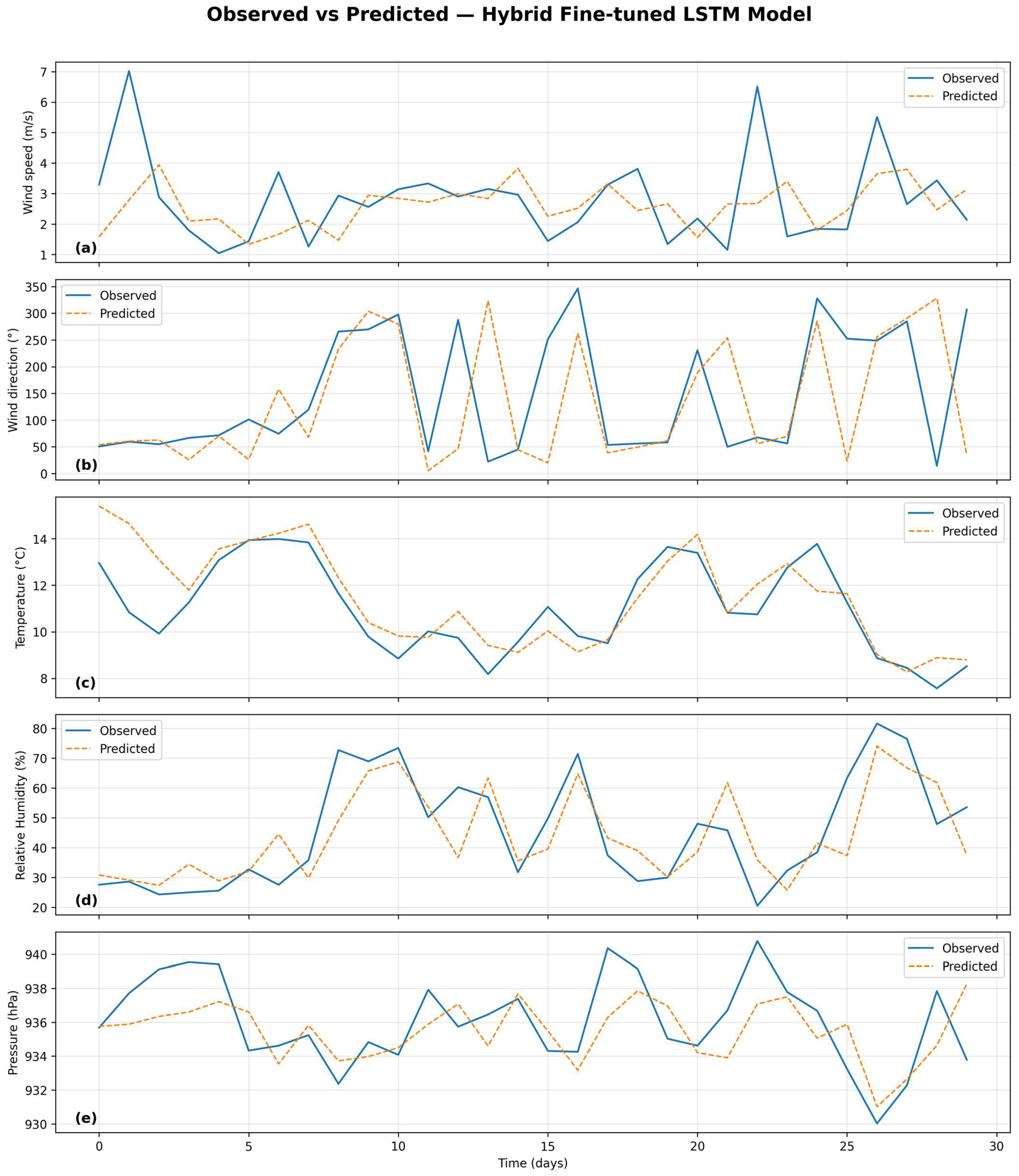
3.3.7. Predicted vs. Observed Series Visualization (Fine-Tuned LSTM)

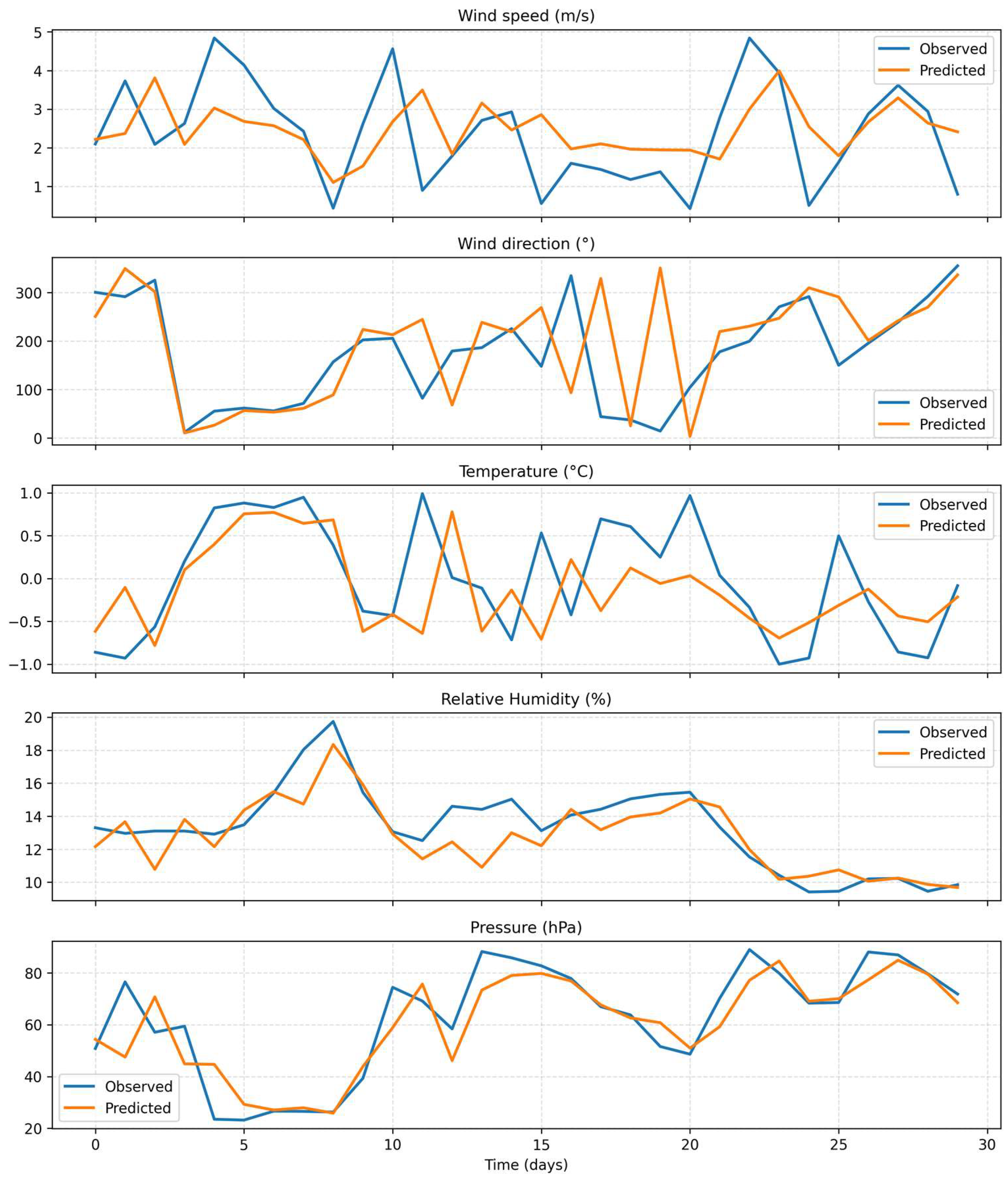
Figure 10 illustrates the comparison between observed and predicted time series for the five analyzed variables—temperature, wind speed, wind direction, relative humidity, and atmospheric pressure—using the fine-tuned LSTM configuration. 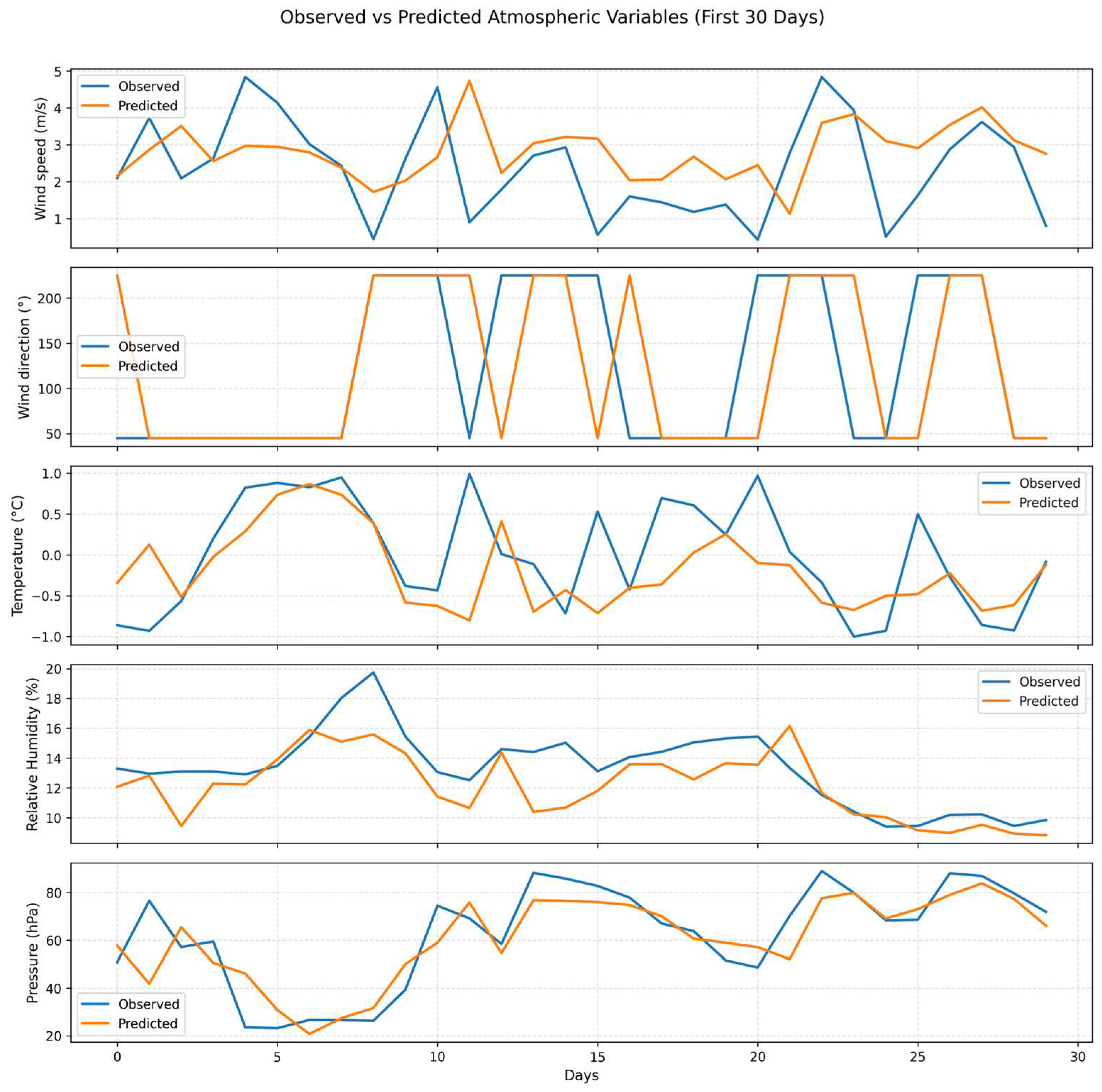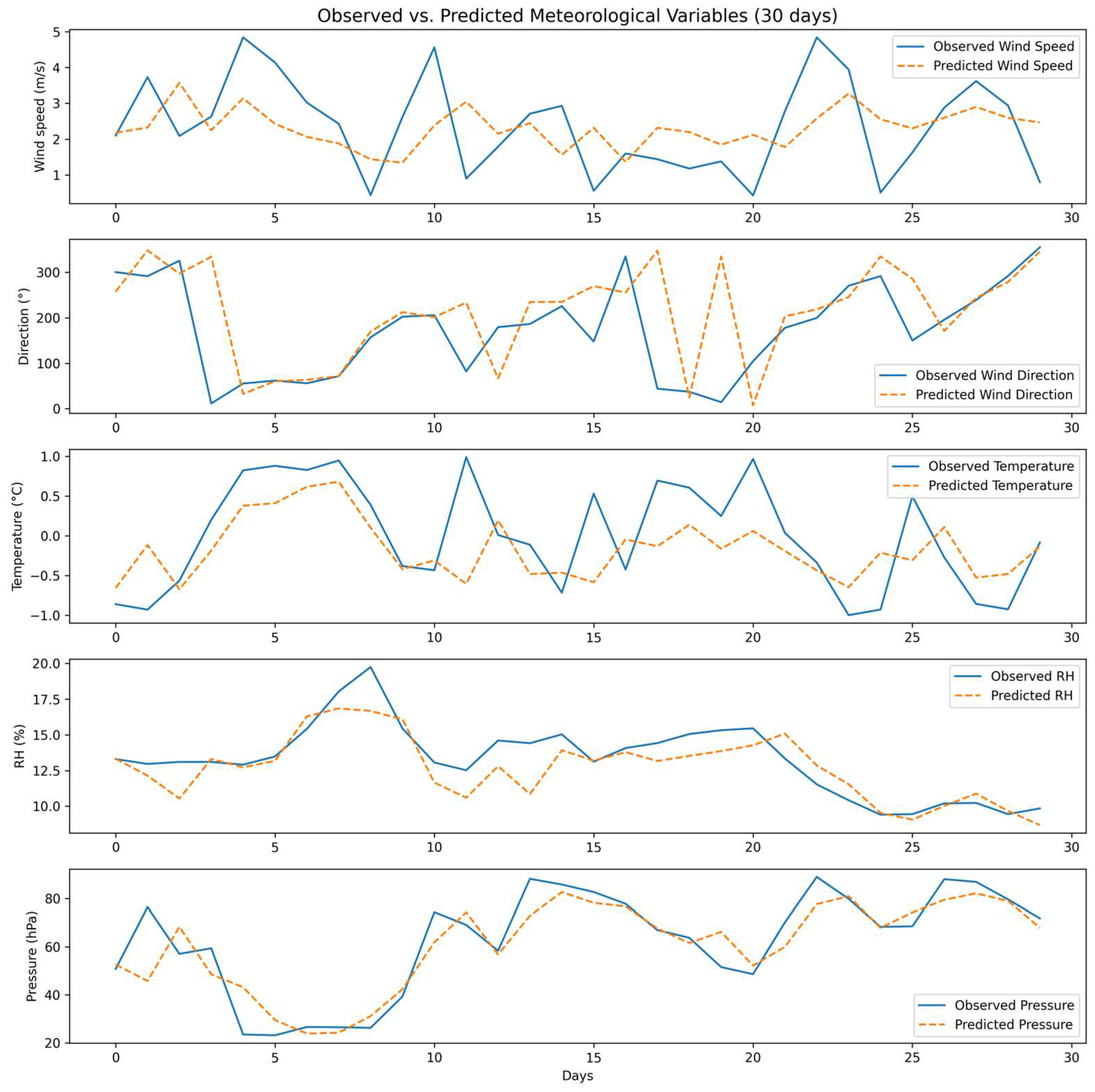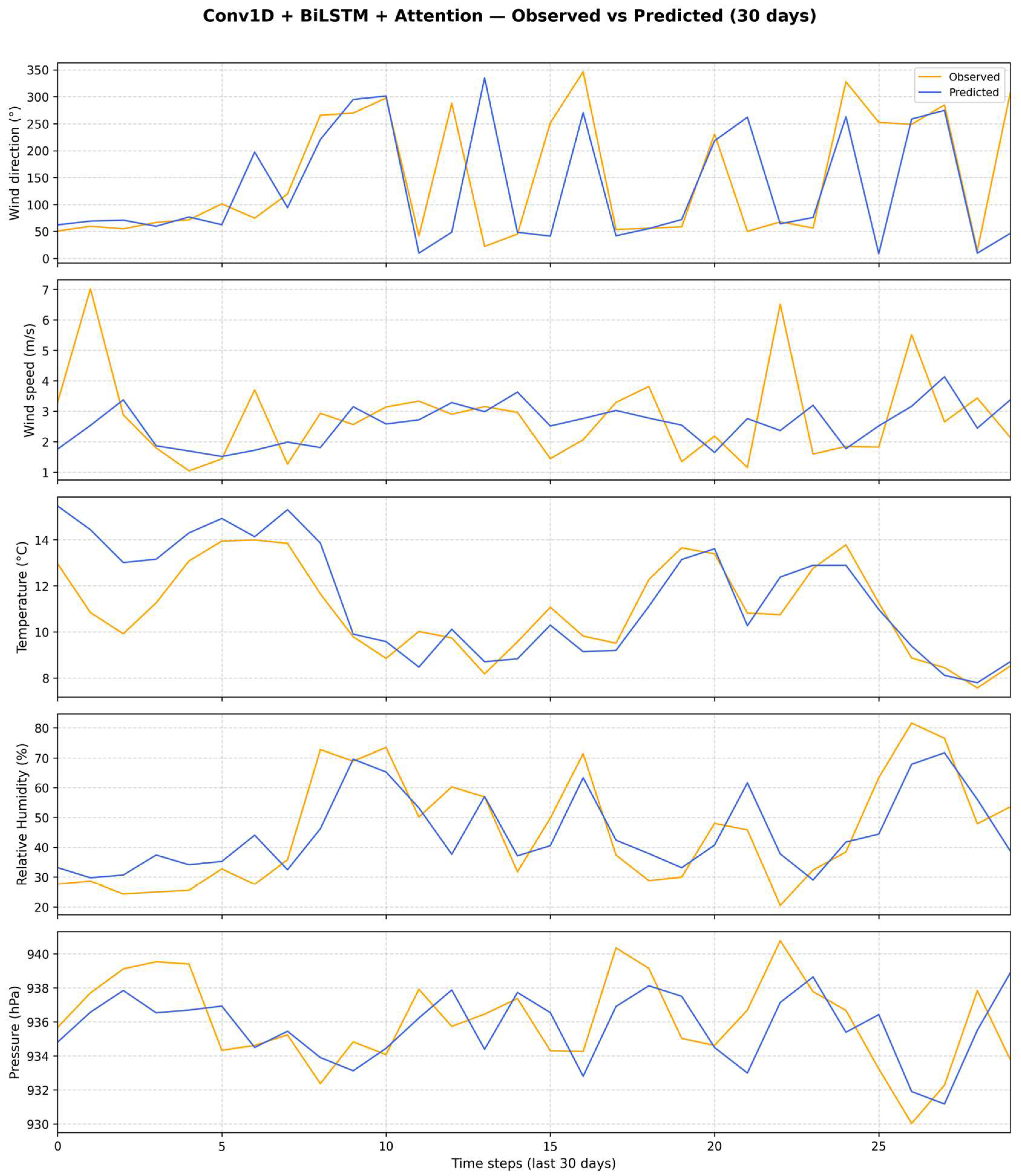This model was selected for graphical representation due to its superior overall performance in terms of RMSE, MAE, and R² (Table 4, Table 5, Table 6, Table 7 and Table 8). For completeness, the corresponding predicted–observed panels for the remaining models (LSTM, CNN + LSTM, BiLSTM + Attention, and Conv1D + BiLSTM + Attention) are provided in Appendix A.2. Predicted vs. Observed Panels for Meteorological Variables (Figure A5, Figure A6, Figure A7 and Figure A8).

The predicted series exhibit strong agreement with the observed values, accurately reproducing both short-term fluctuations and long-term seasonal trends. For temperature and relative humidity, the alignment is particularly close, reflecting the model’s ability to capture variables with high temporal autocorrelation. Wind speed and direction show greater variability and localized discrepancies, primarily during intense Santa Ana wind episodes, which are inherently more difficult to model due to their transient and nonlinear nature. Atmospheric pressure predictions maintain stable coherence with observations, confirming the model’s capacity to represent low-frequency dynamics.

Overall, the graphical evaluation supports the quantitative findings, demonstrating that the fine-tuned LSTM effectively captures the coupled temporal behavior of the atmospheric system at the Agua Caliente station. Minor deviations during extreme events highlight the persistent challenge of data imbalance—only ~2.5% of days correspond to Santa Ana conditions—but do not compromise the model’s general predictive skill. These visual results further reinforce the advantages of the hybrid fine-tuning approach, which improved temporal generalization while maintaining smooth learning dynamics, as shown in the loss curves (Figure 9). The consistency between the graphical and statistical evidence underscores the robustness of the LSTM-based modeling framework for short-term meteorological forecasting under local climatological variability.

3.3.8. Comparative Assessment and Discussion

Overall, the results demonstrate that the recurrent-based deep learning models (LSTM, fine-tuned LSTM, and BiLSTM + Attention) provided the most consistent and accurate predictions across all meteorological variables. Temperature exhibited the highest predictability, with all architectures achieving R² values above 0.91, reflecting the strong temporal continuity and smooth diurnal cycle characteristic of this variable. Wind-related variables, in contrast, showed greater modeling challenges due to their higher short-term variability and nonlinear dynamics. The angular MAE of ~34° obtained for wind direction represents a satisfactory performance within the context of a multivariate configuration with limited predictors, indicating that the attention mechanism effectively enhanced temporal feature representation.

For wind speed, the fine-tuned LSTM outperformed all other models, particularly when emphasizing high-intensity events associated with Santa Ana conditions. This result highlights the benefits of weighted training for capturing rare but critical phenomena. In the case of relative humidity and atmospheric pressure, both variables showed moderate variability and strong autocorrelation, allowing recurrent architectures to efficiently model their temporal evolution. The marginal advantage of attention-based and convolutional components for these variables suggests that simpler recurrent structures can adequately capture their underlying low-frequency patterns.

Overall, these findings reveal that model performance strongly depends on the temporal structure and physical behavior of each variable. Recurrent neural architectures proved to be robust and generalizable for most meteorological variables, while attention mechanisms and adaptive weighting provided additional gains for highly dynamic processes such as wind speed and direction. This supports the use of hybrid and fine-tuned LSTM configurations for multivariate forecasting in regions influenced by complex local circulations, such as the Santa Ana winds.

3.4. Fractal Analysis

The Hurst exponent values estimated for the observed series (1980–2020) (

Table 9. Hurst exponent values $\left(\mathrm{H}\right)$ estimated for the observed meteorological series (1980–2020) and for the predicted outputs of the five deep learning models (LSTM fine-tuned, CNN + LSTM, LSTM, BiLSTM + Attention, and Conv1D + BiLSTM + Attention). The comparison between $\mathrm{H}\mathrm{o}\mathrm{b}\mathrm{s}$ and $\mathrm{H}\mathrm{p}\mathrm{r}\mathrm{e}\mathrm{d}$ provides insight into each model’s ability to preserve the long-term persistence structure of the original time series.

	Serie 1980–2020	LSTM Fine-Tuned		CNN + LSTM		LSTM		BILSTM + Attention		Conv1D + BiLSTM + Attention
Variables	Hurst Exponent	H_obs (Test)	H_pred (Test)	H_obs (Test)	H_pred (Test)	H_obs (Test)	H_pred (Test)	H_obs (Test)	H_pred (Test)	H_obs (Test)	H_pred (Test)
Humidity relative	0.812	0.492	0.489	0.492	0.494	0.492	0.503	0.492	0.505	0.492	0.482
Pressure	0.789	0.474	0.454	0.474	0.413	0.474	0.487	0.474	0.448	0.474	0.42
Temperature	0.932	0.353	0.315	0.353	0.294	0.353	0.323	0.353	0.327	0.353	0.286
Wind direction	0.748	NA *	NA	NA	NA	NA	NA	NA	NA	NA	NA
Wind speed	0.647	0.485	0.506	0.485	0.504	0.485	0.511	0.485	0.513	0.485	0.499

* The Hurst exponent for wind direction could not be computed (NA) due to discontinuities in the angular signal at 0°/360°. Although the series was reconstructed from sine and cosine components to ensure continuity in the prediction phase, this transformation was not suitable for direct Hurst exponent estimation.

) reveal a clear temporal persistence across all meteorological variables, with H > 0.5. Temperature (H = 0.932) and relative humidity (H = 0.812) exhibit the strongest long-term dependence. When comparing these values with those derived from the predicted series of the different models, it is observed that the Hpred values tend to be lower than those of the observed data, suggesting that the models partially reduce the memory or temporal dependence of the original variables.

Among the analyzed variables, wind speed and pressure show the closest agreement between observed and predicted exponents, with differences below 0.03, indicating that the models consistently reproduce the persistence structure of these time series. In contrast, temperature exhibits the largest discrepancies, particularly in the Conv1D + BiLSTM + Attention model, where the Hurst exponent decreases to 0.286, implying a significant loss of long-range correlation. Relative humidity maintains a stable behavior across models, with Hpred values around 0.49, suggesting that the neural networks partially capture the persistence dynamics but fail to fully reproduce the temporal structure of the historical series.

Overall, the results presented in Table 9 confirm that although hybrid architectures (CNN + LSTM and BiLSTM + Attention) demonstrate competitive performance, the Hurst exponent estimates indicate a general tendency to smooth internal variability and to weaken the long-term dependence inherent in the original meteorological records.

These findings highlight that deep learning models can effectively reproduce short-term fluctuations and overall variability in atmospheric variables; however, they tend to underestimate the long-term memory embedded in the original climatic records. The reduction in the Hurst exponent in the predicted series suggests that, while the models capture deterministic dependencies, they partially lose the stochastic persistence associated with multifractal scaling. This limitation indicates that hybrid and attention-based architectures, despite improving predictive accuracy, may smooth out fine-scale temporal structures that are essential to represent the multifractal nature and long-range correlations of climate dynamics.

3.5. Discussion and Implications

The predictive performance of the tested deep learning architectures showed consistent improvements over the persistence and climatology baselines, particularly for temperature, relative humidity, and wind direction. Among the evaluated models, the BiLSTM–Attention configuration achieved the best overall balance across variables, with an angular MAE of 34.1° and RMSE of 50.9° for wind direction, and R² values of 0.94, 0.76, and 0.65 for temperature, relative humidity, and pressure, respectively. These results indicate a slightly better capacity to capture nonlinear dependencies and bidirectional temporal relationships compared to the standard LSTM. However, the differences among models were relatively small (typically below 3%), suggesting that the overall predictive skill is more constrained by the intrinsic characteristics of the dataset—such as the smoothing inherent in the MERRA-2 reanalysis—than by architectural complexity. Therefore, while hybrid structures like CNN–LSTM or BiLSTM–Attention can marginally enhance robustness and temporal coherence, the single-layer LSTM already provides a solid baseline for multivariate meteorological forecasting under Santa Ana wind conditions.

The comparative evaluation of the different architectures indicates that model performance is primarily constrained by the informational limits of the dataset rather than by architectural complexity. The relatively small differences among the fine-tuned, CNN–LSTM, and BiLSTM–Attention models suggest that all architectures are capable of capturing the dominant temporal dependencies in the meteorological variables. Further improvements are therefore more likely to arise from enhanced data richness—such as higher temporal resolution, longer observation periods, or the inclusion of additional predictors—than from increasing model sophistication.

The smoothing observed in predicted wind velocity peaks highlights a common limitation of LSTM-based approaches when representing extreme or transient phenomena. These models tend to approximate the mean dynamics of the system, especially when trained on limited samples of rare events such as Santa Ana winds. Incorporating pressure gradients, large-scale circulation indices, or reanalysis data at higher spatial and temporal resolutions could help capture these events more sharply by providing additional information about the synoptic-scale forcings driving them.

Despite these limitations, the proposed framework demonstrates valuable potential for environmental and engineering applications. By forecasting key meteorological variables—wind speed, wind direction, temperature, humidity, and pressure—it provides a way to characterize atmospheric conditions associated with Santa Ana events, rather than predicting their occurrence directly. This information is useful for early warning and environmental monitoring systems, as it supports the identification of periods with high fire risk, extreme dryness, and strong winds.

Beyond hazard assessment, the model can also support watershed and water resource management by improving the understanding of local climatic dynamics that affect evapotranspiration, soil moisture, and agricultural productivity—particularly in the viticultural regions of northern Baja California. As such, the proposed deep learning framework offers a solid foundation for integrating data-driven forecasting tools into environmental monitoring, risk management, and climate-sensitive engineering practices.

3.6. Limitations and Future Improvements

Several limitations constrain the present study and point to clear avenues for improvement. First, the modeling framework relies exclusively on surface-level reanalysis variables (MERRA-2). Reanalysis products provide spatially continuous and physically consistent fields, but they tend to smooth local extremes and attenuate peak values—particularly for wind speed and pressure—relative to station observations. In contexts where dense in situ networks are unavailable, reanalysis remains a pragmatic and valuable resource, yet its smoothing effect should be acknowledged when interpreting extremes and small-scale variability.

A key extension to improve predictive skill is the incorporation of upper-air (aloft) predictors that describe the vertical and synoptic context driving local conditions. Recommended additional predictors include geopotential height fields (e.g., 500/850 hPa), pressure gradients (horizontal and vertical), planetary boundary layer height (PBLH), layer thickness, and stability indices (e.g., Lifted Index). These variables can provide direct information on the synoptic forcing and vertical structure that govern the onset and intensity of Santa Ana–like episodes and other extreme events.

Other methodological improvements to pursue are: (i) testing higher temporal/spatial resolution reanalysis (e.g., ERA5/ERA5-Land) or assimilating local station data where available; (ii) applying multi-resolution or data-fusion approaches to combine regional reanalysis with downscaled or station observations; (iii) exploring data-augmentation and transfer-learning strategies to better represent rare extreme events; and (iv) validating models extensively against independent local observations to strengthen confidence in extremes. Collectively, these steps would increase physical interpretability and likely improve the models’ ability to predict abrupt, high-impact events that are critical for hydrological applications.

4. Conclusions

This study represents an initial step toward understanding the local atmospheric dynamics associated with Santa Ana wind conditions in the Guadalupe Basin. By applying data-driven deep learning models to surface meteorological variables, the research demonstrates that neural architectures such as LSTM and BiLSTM effectively capture nonlinear dependencies and short-term variability across multiple climatic variables. Among the evaluated models, the fine-tuned LSTM achieved the best overall performance, outperforming persistence and climatology benchmarks for all variables and confirming its capability to generalize complex temporal patterns inherent to regional climate dynamics.

The results indicate that temperature and relative humidity exhibit the highest predictability, whereas wind speed and direction remain more challenging due to their dependence on mesoscale and synoptic processes. These differences underscore the importance of integrating upper-air predictors—such as geopotential height, boundary layer height, and stability indices—in future modeling efforts. Despite the known smoothing limitations of reanalysis products like MERRA-2, their use provides valuable insights in regions with scarce in situ observations, enhancing the understanding of local climatic variability and its linkage to large-scale atmospheric circulation.

From an applied perspective, improving the ability to forecast Santa Ana wind-related meteorological conditions through recurrent neural networks offers tangible benefits for environmental management and risk mitigation. Reliable short-term forecasts can support early warning systems, improve wildfire preparedness, and guide resource allocation during high-risk periods.

Ultimately, this research establishes a methodological foundation for developing integrative forecasting frameworks that connect surface meteorological variability with broader circulation patterns. It contributes to the regional characterization of Santa Ana dynamics and strengthens the scientific basis for sustainable water and climate management in semi-arid basins of northwestern Mexico.