Long-Term Temporal Analysis of Climate Variables for Erzurum

Abstract

The study aims to analyze the long-term trends of climate variables in Erzurum, Türkiye. Trend analyses were conducted on the maximum, minimum, and average temperature and total precipitation series for a 96-year period covering the period 1929–2024. Annual, seasonal, and monthly time series of the variables were illustrated along with their linear trends. Statistical analysis was conducted using the Mann–Kendall test and Sen’s innovative trend analysis methods. The Mann–Kendall test Z-statistic results were evaluated at the 90%, 95%, and 99% significance levels. Maximum temperature series show increasing trends in all months except November, December, January, and February and on the annual scale at the α = 0.01 significance level. Minimum temperature series show decreasing trends for all time periods except March and April. The average temperature variable shows no trend in the annual, summer, and winter series, increasing in spring, March, and April (α = 0.05) and decreasing in November (α = 0.1). Trend analysis of the precipitation series indicates a decreasing trend in winter snowfall, as well as in March and June precipitation. Sen’s methodology, in addition to trend indicators, offers a layered assessment opportunity for any time series, with subcategorization based on the magnitude of the data values. According to annual average values, the diurnal temperature range was determined as 11.3 °C in 1929 and 13.5 °C in 2024. Important findings have been obtained for determining sustainable resource management strategies through the monitoring of climate variables.

1. Introduction

The IPCC [1] states that climate change affects the hydrological cycle at local and global scales, causing changes in the frequency and duration of precipitation patterns and leading to extreme weather events such as floods, droughts, and temperature increases. Therefore, analyzing long-term trends in climate variables is crucial not only for monitoring and assessing climate change but also for ensuring sustainable resource management and identifying potential adaptation and mitigation strategies.

Many studies have been conducted to measure the temporal and/or spatial patterns and trends of climate variables under the perspective of climate change at the local scale. Cui et al. [2] investigated trends in air temperature and precipitation parameters recorded in the Yangtze River Basin (YRB) in China between 1960 and 2015. They used linear regression (LR) analysis, the Mann–Kendall (MK) test, and Sen’s innovative trend analysis (ITA). They found increasing trends between 0.15 and 0.23 °C in annual maximum, minimum, and average temperatures, but noted no significant trend in precipitation changes. Another study conducted on the spatial and temporal analysis of precipitation and drought conditions in southwestern Xinjiang [3], China, shows that precipitation is decreasing, and drought tendency is increasing in the study area.

Two separate studies examining temperature and precipitation records from Guwahati, Assam, India, over 50 years [4] and from Kashmir, Kashmir, over 40 years [5], reported increasing temperature trends at all stations, according to the MK and ITA tests. The annual seasonal precipitation trends are increasing in the former and decreasing in the latter. In the rainfall trend analysis based on 102 years of records of the Sindh River basin of India [6], annual and seasonal increasing trends have determined.

A study conducted for Serbia in Europe using MK and ITA trend analysis tools noted increasing trends in annual and seasonal minimum and maximum air temperature series, while no significant trends were identified in summer and winter precipitation series [7]. Similarly, studies conducted for Greece [8], Switzerland and Italy in Europe analyzed trends in climate variables, reporting a decreasing trend in spring precipitation in the Pieria region of Greece, while temperatures in Swiss [9] showed a clear upward trend. It has been shown that the annual maximum precipitation in the Campania region of Italy has no statistically significant trend at most of the recorded stations [10].

The most important common feature of the studies mentioned above, which focused on temperature and precipitation trends in specific regions of Asia and Europe, is the identification of increasing trends in temperature series. Unfortunately, some trend studies conducted in other regions of the globe have also produced similar results. For example; a study investigating the temporal trends of the maximum and minimum temperature series covering the 48 states in the USA from 1895 to 2017 found significant positive trends in both maximum and minimum temperatures [11]. A study examining annual rainfall periods in the Aguascalientes region of Central Mexico using spectral analysis found that annual rainfall has periodicities of 3, 5, 8, 13, and 21 years [12]. A study conducted a temporal and spatial analysis of temperature trends and climate change projections for a river basin in Ethiopia highlighted increasing temperature trends [13]. According to annual and monthly rainfall trends in the Sinjar Region of Iraq, positive trends were recorded in October and April, and negative trends were recorded in the other months [14]. A comprehensive study of temperature and precipitation trends and future projections in eastern and western Mazandaran Province of Iran also identified increasing trends for both parameters [15].

Similar studies to those conducted in many regions of the world to determine the temporal and/or spatial trends of climate variables have been conducted for many cities or regions in Türkiye [16,17,18,19,20,21,22]. One of the earliest studies, conducted by Türkeş in 1996 [16], determined the temporal and spatial trends of annual precipitation changes in Türkiye. Although slight decreases were detected in the area-averaged annual precipitation series, the results of the MK test indicated that the decreasing trends in the precipitation series were not statistically significant. A study analyzing precipitation and drought trends in the Aegean Region for the period 1960–2013 used records from eight stations and reported that monthly precipitation trends decreased across the region in December, January, February, and March [17]. A study on seasonal rainfall variability in the Konya Basin revealed positive winter and summer precipitation and negative spring precipitation trends in the basin between 1971 and 2020 [19]. In another study, the precipitation and temperature trends of the Antalya Basin were examined by the Frequency-Incremental Trend Analysis (F-ITA) method, and it was shown that there were increasing frequency trends in temperatures but no trend in the precipitation series [21].

In all of the studies mentioned above, the selection of temperature and precipitation (and/or drought) parameters to measure temporal and/or spatial patterns and trends in climate variables is undoubtedly no coincidence. Precipitation and temperature are the most important physical variables [4] that determine a region’s climatic conditions, water supply, floods and water scarcity [23,24], agricultural production, and food supply [25,26]. The most commonly used tools to detect temporal trends of these variables are LR, MK test, Sen’s ITA approach [2,3,4,5,6,7,8] and its other versions such as innovative polygon trend analysis (IPTA) [19,21,27,28], Spearman rho [29,30,31], wavelet analysis [32] and machine learning [23,33].

The primary objective of this article is to conduct a trend analysis of temperature and precipitation variables for the city of Erzurum, Türkiye, over a long period of 96 years, supplementing the classical MK trend detection test with the Sen’s ITA approach. The city is located at an average elevation of 2000 m above sea level, one of the highest settlements in Türkiye. The Erzurum basin’s rich groundwater and surface water resources are fed by its unique geomorphology, largely composed of mountains and plateaus, and by its harsh continental climate [34]. In the literature searches conducted during the study period, no comprehensive study examining the trends in climate variables of the region was coincided. Considering the pressure that climate change creates, especially on water resources, a comprehensive study to be conducted on the temporal trend analysis of climate variables in the province is important in terms of providing unique findings for both the scientific literature and climate change strategists.

The results obtained from the temporal trend analysis of climate variables in this city, located in northeastern Türkiye at an average elevation of 2000 m above sea level, are significant because they offer unique findings for both the literature and climate change strategists, as they have not been previously investigated.

2. Materials and Methods

2.1. Study Area and Data

Erzurum is in the north-east of Turkey and is the fourth largest city in the country with a surface area of approximately 25,000 km². The city is located between 40°14′15″ and 42°33′35″ east longitudes and 40°54′57″ and 39°06′10″ north latitudes (Figure 1a,b). Approximately 64% of its surface morphology consists of mountains and the rest of it consists of high plateaus. It is established between 1850 and 2200 m above sea level and, due to its distance from the sea of approximately 377 km, it has climate characteristics of dry and hot summers and long and cold winters. According to the Köppen–Geiger climate classification, the Dfb climate type prevails in the city [35]. According to long-term (1929–2024) statistics, the average daily sunshine duration is 7.0 h, and the average annual temperature, average number of rainy days, and average precipitation are recorded as 5.8 °C, 121.8, and 430.9 mm, respectively [36].

After a long and cold winter, melting snow is the most important source of water for the city’s surface and groundwater resources. Approximately 72% of the water sourced from groundwater (80.21 million m³/year) is used for agricultural irrigation, and 0.02% (2.60 million m³/year) for industrial activities. The remainder is allocated for drinking and livestock farming. 820 MW of electricity is generated from 30 hydroelectric power plants with a total installed capacity of 2500 GWh on the water resources [37].

In this study, daily maximum temperature (T_max,°C), minimum temperature (T_min,°C), and total precipitation (PREP, mm) values covering the 96-year long period between 1 January 1929, and 31 December 2024, were obtained from the records of the Erzurum Airport Station (station id: 17096) of the General Directorate of Meteorology [38]. The latitude and longitude information of the station (Figure 1b,c) located at an altitude of 1758 m are stated as 39.95 and 41.19, respectively [39]. This station was chosen because it has the oldest meteorological records in the city. The area where the station is located is close to the airport and the station is approximately 8.5 km from the city center and also 3.5 km from the nearest residential area.

Firstly, quality controls were performed on the data and missing data were completed. There are only 38 missing data points from each of the maximum and minimum temperature data provided by the station, and 26 missing data points from the total daily precipitation data. Missing values, corresponding to 0.07% and 0.1% of the total number of data points (35,063), were filled in using the arithmetic mean of the values before and after the missing value [40]. This method can provide reliable estimates in cases where spatial variability of the meteorological variable is absent [41].

Daily data were converted to monthly, seasonal and annual values by averaging for T_max and T_min and taking total precipitation values for PREP. Seasons in the study were defined as follows: spring (March–May), summer (June–August), autumn (September–November), and winter (December–February). Average temperatures were calculated from the average of minimum and maximum temperatures [T_mean = (T_max + T_min)/2] [42,43].

2.2. Run Homogeneity Test

Before trend analysis, homogeneity tests were conducted separately for monthly, seasonal and annual [44] average data. As in many studies investigating trend analysis in time and precipitation series for homogeneity, Refs. [28,45,46,47,48] the run homogeneity test [49] was used. The Run (Swed-Eisenhart) test can be used to test two hypotheses: assuming the data to be examined come from the same population (H₀) and are independent (H₁), or vice versa. A time series with a total number of data points N is generally truncated at the median value, and the number of data points below (N_i) and above (N_j) this level is determined. The run test statistic, Z_r, is calculated using Equation (1), where r is the number of runs.

$$Z_r={\displaystyle \frac{r-\frac{2N_i{N}_j}{N_i+N_j}+1}{\sqrt{\frac{2N_i{N}_j(2N_i{N}_j-N)}{N^2(N-1)}}}}$$

(1)

If the Z_r value is less than the critical z value of the two-sided hypothesis test, the H₀ hypothesis, which indicates that the time series under study is statistically significantly homogeneous, is accepted. Otherwise, it is rejected, and therefore, the H₁ hypothesis, which indicates that the series is not homogeneous, is accepted.

2.3. Mann–Kendall (MK) Test

This nonparametric statistical method, proposed by Mann [50] and revised by Kendall [51], is used to identify trends in time series of hydrological and climatic variables. While it effectively detects increasing or decreasing monotonic trends in the series, it does not provide information about whether the trend is linear. The test statistic S, given by Equation (2), is positive, indicating an increasing trend, negative, indicating a decreasing trend, and equal to 0 when no trend is present.

$$S=\sum _{i=1}^{n-1}\sum _{j=i+1}^{n}sgn(x_j-x_i)$$

(2)

$$sgn\left(x_j-x_i\right)=\left\{\begin{array}{c}1 ; if(x_j-x_i)>0\\ 0 ; if(x_j-x_i)=0\\ -1 ; if(x_j-x_i)<0\end{array}\right.$$

(3)

where n is the data length and x_i and x_j represent the data values at time i and j, respectively. The variance of S, Var(S), can be calculated as follows:

$$Var\left(S\right)={\displaystyle \frac{1}{18}}\left[n\left(n-1\right)\left(2n+5\right)-\sum _{i=1}^p{t}_i\left(t_i-1\right)\left({2t}_i+5\right)\right]$$

(4)

In Equation (4), p is the number of connected groups and t_i is the number of repetitions of the data set. The Z statistic or Standard Normal Variable used to evaluate the significance of the trend is calculated using the following Equation (5):

$$Z=\left\{\begin{array}{c}{\displaystyle \frac{S-1}{\sqrt{Var\left(S\right)}}}; if S>0\\ 0; if S=0\\ {\displaystyle \frac{S+1}{\sqrt{Var\left(S\right)}}}; if S<0\end{array}\right.$$

(5)

The calculated Z statistic is evaluated by comparing it with the critical z value in the standard normal table for the determined significance level (α). If the absolute Z value is greater than the critical z value, the trend is statistically significant, and the H₀ hypothesis is rejected. H₀, the initial hypothesis, and H₁, the alternative hypothesis, are constructed as follows:

Hypothesis 1. 

H₀: “There is no trend in the series”.

Hypothesis 2. 

H₁: “There is a trend in the series”.

In this study, the evaluations were made based on significance levels of 90%, 95%, and 99% (α = 0.10, α = 0.05, and α = 0.01, respectively). α = 0.05 is a generally accepted significance level that balances reliability. α = 0.01 indicates a stronger significance level, which also reduces false positives, and α = 0.1 indicates a lower significance level, which can identify weak trends. Since the dataset had a sample size of more than 50 (35,063) and a high slope (≥0.01), no pre-whitening was applied to the data before testing [52].

2.4. Sen’s Innovative Trend Analysis (ITA)

According to the method developed by Şen [53], whose deterministic background is explained in detail [54], the time series is initially divided into two equal parts. The first half-series can be represented as x_i (i = 1, 2, …, n/2) and the second half-series as x_j (j = n/2 + 1, n/2 + 2, …, n). Each half-series is sorted from smallest to largest, and the second half-series is plotted against the first half-series as a scatter plot in a Cartesian coordinate system. The position of the scatter plot relative to a 45° line (1:1 line) inserted into the coordinate plane can be used to evaluate the trend of the time series. According to the graph presented in Figure 2, it is possible to identify five different trends in the time series: monotonic increase (or decrease), non-monotonic increase (or decrease), and trendless.

The plot area can be divided into an appropriate number of main grids and categorized as “very low (VL)”, “low (L)”, “medium (M)”, “high (H)” and “very high (VH)”. This approach can help visualize and evaluate smaller-scale trend changes in the series. The ordering starts from the origin (“very low”) and progresses sequentially toward the positive end of the y-axis. Therefore, stronger trend effects emerge as one moves to the up the scatterplot. For further reading, see Şen’s studies [53,54,55].

In the analysis, Sen’s slope can be calculated as given in Equation (6). In the equation, ${\overline{x}}_1$ and ${\overline{x}}_2$ are equal to the arithmetic mean of the first and second half series, respectively.

$$\mathit{\text{Sen’s slope}}={\displaystyle \frac{2\left({\overline{x}}_2-{\overline{x}}_1\right)}{n}}$$

(6)

In this study, MK test, Sen’s slope and related statistics for monthly, seasonal, and annual series were calculated using R command. Data quality control and editing was done via MS Office 365 Excel, and data visualization was done using Origin 2024.

3. Results

Daily values of temperature (T_max, T_min, T_mean) and total precipitation (PREP) variables for Erzurum over the long period from 1929 to 2024 were converted to monthly values. According to the results of the run homogeneity test applied to the data series, all series are homogeneous. The homogeneity test results and descriptive statistics for the monthly values are presented separately in

Table A1. The results of the runs test.

	Tmax						Tmin						Precipitation
	Ni	Nj	N	r	Zr	Hypothesis *	Ni	Nj	N	r	Zr	Hypothesis *	Ni	Nj	N	r	Zr	Hypothesis *
January	46	50	96	44	−0.006	H0	48	48	96	44	−0.006	H0	60	36	96	44	0.000	H0
February	51	45	96	54	0.016	H0	44	52	96	54	0.016	H0	59	37	96	54	0.022	H0
March	51	45	96	58	0.024	H0	48	48	96	58	0.024	H0	55	41	96	58	0.027	H0
April	53	43	96	56	0.021	H0	47	49	96	56	0.019	H0	58	38	96	56	0.025	H0
May	49	47	96	48	0.002	H0	48	48	96	48	0.002	H0	54	42	96	48	0.004	H0
June	50	46	96	38	−0.019	H0	45	51	96	38	−0.019	H0	48	48	96	38	−0.019	H0
July	52	44	96	45	−0.004	H0	48	48	96	45	−0.004	H0	57	39	96	45	−0.001	H0
August	51	45	96	40	−0.015	H0	46	50	96	40	−0.015	H0	61	35	96	40	−0.008	H0
September	48	48	96	42	−0.011	H0	42	54	96	42	−0.009	H0	57	39	96	42	−0.007	H0
October	51	45	96	48	0.003	H0	46	50	96	48	0.002	H0	53	43	96	48	0.003	H0
November	45	51	96	46	−0.002	H0	46	50	96	46	−0.002	H0	54	42	96	46	−0.001	H0
December	47	49	96	46	−0.002	H0	47	49	96	46	−0.002	H0	55	41	96	46	0.000	H0
Spring	51	45	96	50	0.007	H0	47	49	96	50	0.007	H0	55	41	96	50	0.009	H0
Summer	53	43	96	30	−0.036	H0	47	49	96	30	−0.037	H0	55	41	96	30	−0.035	H0
Fall	47	49	96	42	−0.011	H0	43	53	96	42	−0.010	H0	55	41	96	42	−0.009	H0
Winter	55	41	96	42	−0.009	H0	46	50	96	42	−0.011	H0	58	38	96	42	−0.007	H0
Annual	50	46	96	36	−0.024	H0	46	50	96	36	−0.024	H0	55	41	96	36	−0.022	H0

* The significance level α = 0.05 critical z = ±1.960.

,

Table A2. The descriptive statistics for monthly, seasonal and annual trends of T_max in Erzurum for the period from 1929 to 2024.

	Min	Max	Mean	sd
January	−10.0	2.7	−3.8	2.7
February	−8.0	4.2	−2.2	2.7
March	−3.3	11.3	2.7	3.2
April	4.1	18.0	11.1	2.6
May	13.2	21.9	16.9	1.7
June	18.4	27.2	21.9	1.9
July	22.4	31.9	26.6	1.8
August	23.3	31.7	27.3	1.9
September	18.1	27.6	22.7	2.0
October	8.8	20.3	15.2	2.0
November	−0.1	12.8	6.9	2.7
December	−8.1	5.7	−0.9	3.1
Spring	6.1	15.0	10.3	1.8
Summer	21.8	28.7	25.3	1.5
Fall	12.1	18.7	14.9	1.5
Winter	−7.7	2.8	−2.3	1.9
Annual	9.5	15.3	12.0	1.2

,

Table A3. The descriptive statistics for monthly, seasonal and annual trends of T_min in Erzurum for the period from 1929 to 2024.

	Min	Max	Mean	sd
January	−23.4	−3.4	−13.9	3.9
February	−22.9	−4.9	−12.5	4.0
March	−18.8	−0.3	−7.0	3.6
April	−4.5	3.0	0.1	1.6
May	1.2	7.5	4.3	1.4
June	3.7	10.3	7.3	1.4
July	6.9	14.3	11.1	1.5
August	7.3	15.2	11.2	1.6
September	1.5	10.8	6.4	2.0
October	−4.1	5.4	1.7	2.0
November	−12.1	0.8	−3.8	2.8
December	−20.5	−3.6	−10.2	4.0
Spring	−6.3	1.9	−0.9	1.6
Summer	6.9	12.2	9.9	1.3
Fall	−4.6	5.4	1.4	1.9
Winter	−20.5	−5.0	−12.2	3.0
Annual	−5.0	2.8	−0.4	1.6

,

Table A4. The descriptive statistics for monthly, seasonal and annual trends of T_mean in Erzurum for the period from 1929 to 2024.

	Min	Max	Mean	sd
January	−16.7	−0.6	−8.9	3.2
February	−14.9	−0.4	−7.4	3.2
March	−10.2	5.0	−2.1	3.3
April	−0.2	9.8	5.6	1.9
May	8.2	14.1	10.6	1.1
June	12.2	17.9	14.6	1.2
July	16.2	22.2	18.8	1.2
August	16.7	22.7	19.3	1.3
September	11.5	18.9	14.6	1.5
October	4.0	12.1	8.5	1.5
November	−5.7	6.3	1.5	2.5
December	−14.0	−0.3	−5.6	3.4
Spring	1.1	7.9	4.7	1.5
Summer	15.4	19.6	17.6	0.9
Fall	4.5	11.3	8.2	1.3
Winter	−13.8	−1.6	−7.3	2.4
Annual	2.3	8.3	5.8	1.1

and

Table A5. The descriptive statistics for monthly, seasonal and annual trends of PREP in Erzurum for the period from 1929 to 2024.

	Min	Max	Mean	sd
January	1.7	85.6	21.5	15.9
February	1.2	90.0	25.4	16.7
March	1.2	91.2	35.5	17.1
April	8.8	150.2	54.6	28.9
May	12.1	186.9	73.1	32.8
June	2.9	112.6	48.5	25.1
July	0.0	173.6	28.3	24.8
August	0.0	63.0	17.6	16.5
September	0.0	103.1	24.1	20.0
October	0.0	210.8	46.3	34.8
November	0.0	106.7	32.9	21.0
December	2.1	93.4	22.0	13.8
Spring	69.7	333.7	163.2	49.8
Summer	18.4	225.2	94.4	44.5
Fall	26.4	249.1	103.3	43.8
Winter	17.1	189.5	68.9	32.2
Annual	202.4	829.6	429.9	106.6

in Appendix A.

Annual, seasonal, and monthly trend analyses for monthly mean T_max, T_min, T_mean, and total precipitation were conducted separately using the MK test and Sen’s ITA approach. To ensure a combined evaluation of the results of the temporally layered analyses, the MK test results are summarized in

Table 1. MK trend analysis results.

		MK Test Statistic	Z	H0 Hypothesis /Trend (±)			MK Test Statistic	Z	H0 Hypothesis /Trend (±)
January	Tmax	251.0	0.79	Accept ▬	October	Tmax	1081.0	3.42 **	Reject ▲
	Tmin	−619.0	−1.96 **	Reject ▼		Tmin	−1512.0	−4.78 ***	Reject ▼
	Tmean	−224.0	−0.71	Accept ▬		Tmean	−332.0	−1.05	Accept ▬
	PREP	−829.0	−2.62 **	Reject ▼		PREP	−217.0	−0.68	Accept ▬
February	Tmax	210.0	0.66	Accept ▬	November	Tmax	469.0	1.48	Accept ▬
	Tmin	−658.0	−2.08 **	Reject ▼		Tmin	−1468.0	−4.64 ***	Reject ▼
	Tmean	−310.0	−0.98	Accept ▬		Tmean	−570.0	−1.80 *	Reject ▼
	PREP	−1169.0	−3.70 ***	Reject ▼		PREP	−523.0	−1.65 *	Reject ▼
March	Tmax	1114.0	3.52 ***	Reject ▲	December	Tmax	48.0	0.15	Accept ▬
	Tmin	405.0	1.28	Accept ▬		Tmin	−732.0	−2.31 **	Reject ▼
	Tmean	775.0	2.45 **	Reject ▲		Tmean	−370.0	−1.17	Accept ▬
	PREP	−697.0	−2.20 **	Reject ▼		PREP	−450.0	−1.42	Accept ▬
April	Tmax	1190.0	3.76 ***	Reject ▲	Spring	Tmax	1520.0	4.81 ***	Reject ▲
	Tmin	−508.0	−1.60	Accept ▬		Tmin	−264.0	−0.83	Accept ▬
	Tmean	640.0	2.02 **	Reject ▲		Tmean	732.0	2.31 **	Reject ▲
	PREP	−172.0	−0.54	Accept ▬		PREP	−295.0	−0.93	Accept ▬
May	Tmax	895.0	2.83 **	Reject ▲	Summer	Tmax	1948.0	6.16 ***	Reject ▲
	Tmin	−1334.0	−4.22 ***	Reject ▼		Tmin	−1620.0	−5.12 ***	Reject ▼
	Tmean	−99.0	−0.31	Accept ▬		Tmean	428.0	1.35	Accept ▬
	PREP	−74.0	−0.23	Accept ▬		PREP	−571.0	−1.80 *	Reject ▼
June	Tmax	1558.0	4.93 ***	Reject ▲	Fall	Tmax	1412.0	4.47 ***	Reject ▲
	Tmin	−1321.0	−4.18 ***	Reject ▼		Tmin	−1826.0	−5.78 ***	Reject ▼
	Tmean	323.0	1.02	Accept ▬		Tmean	−496.0	−1.57	Accept ▬
	PREP	−665.0	−2.10 **	Reject ▼		PREP	−658.0	−2.08 **	Reject ▼
July	Tmax	1631.0	5.16 ***	Reject ▲	Winter	Tmax	302.0	0.95	Accept ▬
	Tmin	−1485.0	−4.70 ***	Reject ▼		Tmin	−816.0	−2.58 **	Reject ▼
	Tmean	349.0	1.10	Accept ▬		Tmean	−426.0	−1.35	Accept ▬
	PREP	−390.0	−1.23	Accept ▬		PREP	−1170.0	−3.70 ***	Reject ▼
August	Tmax	1559.0	4.93 ***	Reject ▲	Annual	Tmax	1756.0	5.56 ***	Reject ▲
	Tmin	−1438.0	−4.55 ***	Reject ▼		Tmin	−1270.0	−4.02 ***	Reject ▼
	Tmean	205.0	0.65	Accept ▬		Tmean	−62.0	−0.19	Accept ▬
	PREP	−202.0	−0.64	Accept ▬		PREP	−917.0	−2.90 **	Reject ▼
September	Tmax	1393.0	4.41 ***	Reject ▲
	Tmin	−1549.0	−4.90 ***	Reject ▼
	Tmean	−254.0	−0.80	Accept ▬
	PREP	−413.0	−1.30	Accept ▬

▲: increase trend. ▼: decrease trend. ▬: trendless 0: no data. * The significance level α = 0.10 critical z = 1.645. ** The significance level α = 0.05 critical z = 1.960. *** The significance level α = 0.01 critical z = 2.575.

, and the ITA results are summarized in

Table 2. ITA results.

		Sen’s Slope	VL	L	M	H	VH			Sen’s Slope	VL	L	M	H	VH
January	Tmax	0.009	▬	▬	▼	▲	▲	October	Tmax	0.023	0	▲	▲	▲	▲
	Tmin	−0.027	▼	▼	▼	▬	▼		Tmin	−0.035	▼	▼	▼	▼	▼
	Tmean	−0.008	▼	▼	▬	▲	▼		Tmean	−0.005	▲	▬	▼	▼	0
	PREP	−0.120	▼	▼	▼	0	0		PREP	−0.079	▲	▬	▼	▬	▼
February	Tmax	0.007	▲	▬	▬	▲	▲	November	Tmax	0.014	▼	▲	▬	▲	▼
	Tmin	−0.034	▼	▼	▼	▼	▬		Tmin	−0.047	▼	▼	▼	▼	▼
	Tmean	−0.012	▼	▼	▼	▲	▲		Tmean	−0.016	▼	▼	▼	▼	▼
	PREP	−0.200	▼	▼	▼	▼	0		PREP	−0.125	▼	▬	▼	▼	0
March	Tmax	0.044	▲	▲	▲	▲	▲	December	Tmax	0.002	▬	▼	▬	▬	▲
	Tmin	0.019	▼	▼	▬	▬	▲		Tmin	−0.034	▼	▼	▼	▼	▼
	Tmean	0.032	▼	▲	▲	▲	▲		Tmean	−0.017	▼	▼	▼	▼	▬
	PREP	−0.130	▼	▼	▼	▼	▼		PREP	−0.053	▼	▼	▲	▼	0
April	Tmax	0.039	▲	▲	▲	▲	▲	Spring	Tmax	0.033	0	▲	▲	▲	▲
	Tmin	−0.010	▲	▼	▼	▼	▼		Tmin	−0.005	▼	▼	▼	▼	▼
	Tmean	0.015	0	▲	▲	▲	▲		Tmean	0.014	▼	▲	▬	▲	▲
	PREP	−0.058	▬	▬	▬	▬	▲		PREP	−0.156	▼	▬	▲	▼	0
May	Tmax	0.018	▬	▲	▲	▲	▲	Summer	Tmax	0.034	0	▲	▲	▲	▲
	Tmin	−0.021	▼	▼	▼	▼	▼		Tmin	−0.023	▼	▼	▼	▼	▼
	Tmean	−0.001	▬	▼	▬	▼	0		Tmean	0.005	▼	▼	▬	▬	▬
	PREP	−0.030	▬	▬	▬	▼	▼		PREP	−0.296	▼	▼	▼	▼	▼
June	Tmax	0.033	▲	▲	▲	▲	▲	Fall	Tmax	0.024	▬	▲	▲	▲	▲
	Tmin	−0.022	▼	▼	▼	▼	▼		Tmin	−0.038	▼	▼	▼	▼	0
	Tmean	0.005	▲	▬	▼	▬	▬		Tmean	0.007	▼	▼	▼	▼	0
	PREP	−0.216	▼	▼	▼	▼	0		PREP	−0.332	▬	▼	▼	▬	▼
July	Tmax	0.033	0	▲	▲	▲	▲	Winter	Tmax	0.006	▼	▬	▬	▲	▲
	Tmin	−0.024	▼	▼	▼	▼	▼		Tmin	−0.030	▼	▼	▼	▼	▼
	Tmean	0.005	▲	▼	▲	▬	▲		Tmean	−0.012	▼	▼	▼	▼	▲
	PREP	−0.088	▬	▼	▼	0	0		PREP	−0.378	▼	▼	▼	0	0
August	Tmax	0.034	▲	▲	▲	▲	▲	Annual	Tmax	0.025	▲	▲	▲	▲	▲
	Tmin	−0.026	▼	▼	▼	▼	▼		Tmin	−0.023	▼	▼	▼	▼	▼
	Tmean	0.004	▼	▲	▼	▲	▼		Tmean	−0.001	▼	▼	▼	▬	▼
	PREP	−0.032	▲	▼	▼	▼	▼		PREP	−1.156	▼	▼	▼	▼	0
September	Tmax	0.032	0	▲	▲	▲	▲
	Tmin	−0.038	▼	▼	▼	▼	▼
	Tmean	−0.005	▼	▼	▼	▬	0
	PREP	−0.073	▼	▼	▼	▼	0

▲: increase trend ▼: decrease trend. ▬: trendless 0: no data. VL: Very low L: Low M: Medium. H: High VH: Very high.

. All of MK test and ITA results can be seen in

Table A6. Results of MK test and ITA for T_max.

				Mann–Kendall Test			ITA
	Z	N	p	S	varS	tau	Sen’s Slope (°C/year)	95 Percent Confidence Interval
January	0.791	96	0.429	251.00	99,812.33	0.055	0.009	−0.011	0.029
February	0.662	96	0.508	210.00	99,811.33	0.046	0.007	−0.015	0.028
March	3.523	96	0.000	1114.00	99,813.33	0.244	0.044	0.021	0.069
April	3.764	96	0.000	1190.00	99,811.33	0.261	0.039	0.020	0.058
May	2.830	96	0.005	895.00	99,810.33	0.196	0.018	0.005	0.030
June	4.928	96	0.000	1558.00	99,813.33	0.342	0.033	0.022	0.046
July	5.159	96	0.000	1631.00	99,810.33	0.358	0.033	0.022	0.045
August	4.932	96	0.000	1559.00	99,812.33	0.342	0.034	0.021	0.046
September	4.406	96	0.000	1393.00	99,812.33	0.306	0.032	0.019	0.046
October	3.419	96	0.001	1081.00	99,807.67	0.237	0.023	0.010	0.038
November	1.481	96	0.139	469.00	99,812.33	0.103	0.014	−0.005	0.035
December	0.149	96	0.882	48.00	99,808.67	0.011	0.002	−0.023	0.027
Spring	4.808	96	0.000	1520.00	99,813.33	0.333	0.033	0.020	0.045
Summer	6.163	96	0.000	1948.00	99,813.33	0.427	0.034	0.025	0.044
Fall	4.466	96	0.000	1412.00	99,813.33	0.310	0.024	0.014	0.034
Winter	0.953	96	0.341	302.00	99,813.33	0.066	0.006	−0.008	0.021
Annual	5.555	96	0.000	1756.00	99,813.33	0.385	0.025	0.017	0.033

,

Table A7. Results of MK test and ITA for T_min.

				Mann–Kendall Test			ITA
	Z	N	p	S	varS	tau	Sen’s Slope (°C/Year)	95 Percent Confidence Interval
January	−1.956	96	0.050	−619.00	99,812.33	−0.136	−0.027	−0.054	0.000
February	−2.080	96	0.038	−658.00	99,813.33	−0.144	−0.034	−0.063	−0.002
March	1.279	96	0.201	405.00	99,812.33	0.089	0.019	−0.008	0.046
April	−1.605	96	0.109	−508.00	99,809.33	−0.111	−0.010	−0.021	0.003
May	−4.219	96	0.000	−1334.00	99,811.33	−0.293	−0.021	−0.030	−0.012
June	−4.178	96	0.000	−1321.00	99,810.33	−0.290	−0.022	−0.032	−0.013
July	−4.697	96	0.000	−1485.00	99,810.33	−0.326	−0.024	−0.034	−0.015
August	−4.549	96	0.000	−1438.00	99,811.33	−0.326	−0.026	−0.037	−0.016
September	−4.900	96	0.000	−1549.00	99,810.33	−0.340	−0.038	−0.050	−0.025
October	−4.783	96	0.000	−1512.00	99,811.33	−0.332	−0.035	−0.050	−0.022
November	−4.643	96	0.000	−1468.00	99,813.33	−0.322	−0.047	−0.067	−0.029
December	−2.314	96	0.021	−732.00	99,813.33	−0.161	−0.034	−0.066	−0.006
Spring	−0.832	96	0.405	−264.00	99,813.33	−0.058	−0.005	−0.016	0.007
Summer	−5.125	96	0.000	−1620.00	99,813.33	−0.355	−0.023	−0.031	−0.015
Fall	−5.777	96	0.000	−1826.00	99,813.33	−0.400	−0.038	−0.050	−0.027
Winter	−2.580	96	0.010	−816.00	99,813.33	−0.179	−0.030	−0.053	−0.008
Annual	−4.017	96	0.000	−1270.00	99,813.33	−0.279	−0.023	−0.034	−0.013

,

Table A8. Results of MK test and ITA for T_mean.

				Mann–Kendall Test			ITA
	Z	N	p	S	varS	tau	Sen’s Slope (°C/year)	95 Percent Confidence Interval
January	−0.706	96	0.480	−224.00	99,813.33	−0.049	−0.008	−0.033	0.015
February	−0.978	96	0.328	−310.00	99,813.33	−0.068	−0.012	−0.040	0.014
March	2.450	96	0.014	775.00	99,812.33	0.170	0.032	0.006	0.055
April	2.023	96	0.043	640.00	99,813.33	0.140	0.015	0.001	0.029
May	−0.310	96	0.756	−99.00	99,812.33	−0.022	−0.001	−0.010	0.008
June	1.019	96	0.308	323.00	99,812.33	0.071	0.005	−0.005	0.014
July	1.102	96	0.271	349.00	99,810.33	0.077	0.005	−0.005	0.014
August	0.646	96	0.519	205.00	99,810.33	0.045	0.004	−0.007	0.014
September	−0.801	96	0.423	−254.00	99,811.33	−0.056	−0.005	−0.017	0.006
October	−1.048	96	0.295	−332.00	99,813.33	−0.073	−0.005	−0.016	0.006
November	−1.801	96	0.072	−570.00	99,811.33	−0.125	−0.016	−0.033	0.001
December	−1.168	96	0.243	−370.00	99,813.33	−0.081	−0.017	−0.045	0.012
Spring	2.314	96	0.021	732.00	99,813.33	0.161	0.014	0.002	0.026
Summer	1.352	96	0.177	428.00	99,812.33	0.094	0.005	−0.002	0.012
Fall	−1.567	96	0.117	−496.00	99,813.33	−0.109	0.007	−0.017	0.002
Winter	−1.345	96	0.179	−426.00	99,813.33	−0.093	−0.012	−0.031	0.005
Annual	−0.193	96	0.847	−62.00	99,813.33	−0.014	−0.001	−0.009	0.008

and

Table A9. Results of MK test and ITA for PREP.

				Mann–Kendall Test			ITA
	Z	N	p	S	varS	tau	Sen’s Slope (mm/year)	95 Percent Confidence Interval
January	−2.621	96	0.009	−829.00	99,800.67	−0.182	−0.120	−0.208	−0.029
February	−3.697	96	0.000	−1169.00	99,809.33	−0.256	−0.200	−0.320	−0.100
March	−2.203	96	0.028	−697.00	99,804.33	−0.153	−0.130	−0.252	−0.017
April	−0.541	96	0.588	−172.00	99,808.33	−0.038	−0.058	−0.260	0.144
May	−0.231	96	0.817	−74.00	99,811.33	−0.016	−0.030	−0.277	0.212
June	−2.102	96	0.036	−665.00	99,801.67	−0.146	−0.216	−0.414	−0.018
July	−1.231	96	0.218	−390.00	99,805.33	−0.086	−0.088	−0.232	0.046
August	−0.636	96	0.525	−202.00	99,803.67	−0.044	−0.032	−0.138	0.058
September	−1.304	96	0.192	−413.00	99,800.67	−0.091	−0.073	−0.200	0.047
October	−0.684	96	0.494	−217.00	99,811.33	−0.048	−0.079	−0.343	0.150
November	−1.652	96	0.098	−523.00	99,807.33	−0.115	−0.125	−0.247	0.025
December	−1.421	96	0.155	−450.00	99,801.67	−0.099	−0.053	−0.143	0.026
Spring	−0.931	96	0.352	−295.00	99,812.33	−0.065	−0.156	−0.527	0.199
Summer	−1.804	96	0.071	−571.00	99,812.33	−0.125	−0.296	−0.604	0.027
Fall	−2.080	96	0.038	−658.00	99,804.67	−0.144	−0.332	−0.640	−0.015
Winter	−3.700	96	0.000	−1170.00	99,804.67	−0.257	−0.378	−0.580	−0.182
Annual	−2.899	96	0.004	−917.00	99,812.33	−0.201	−1.156	−1.882	−0.416

in the Appendix A.

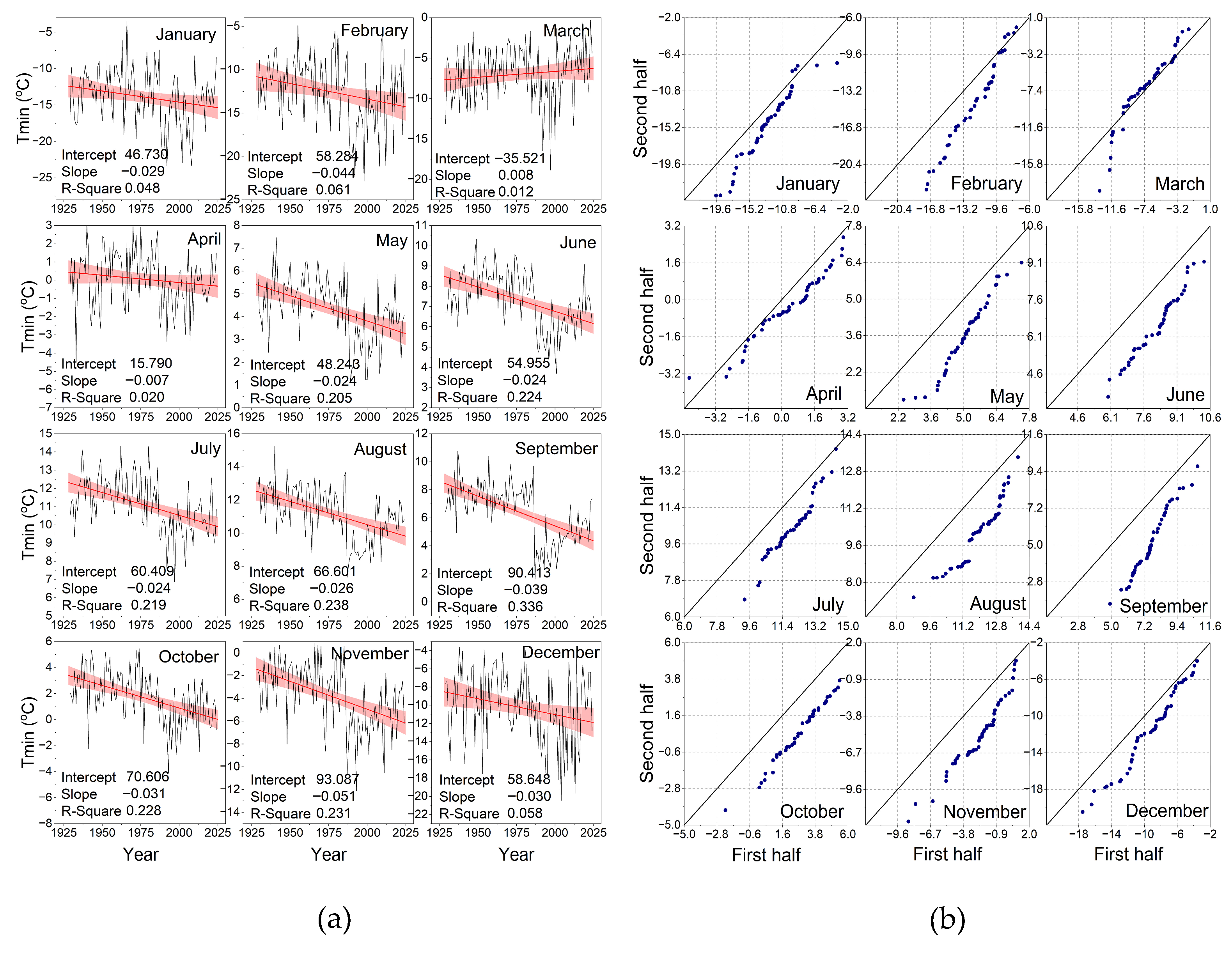
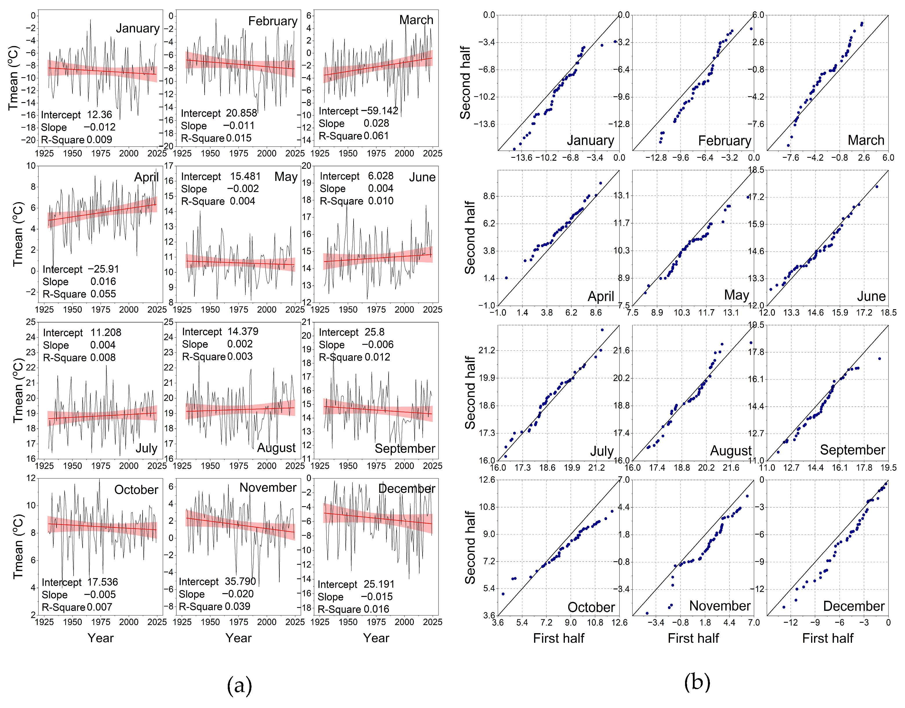
Along with ITA charts, time series trends over a 96-year period and linear fit analyses for these trends are also displayed on the chart. This allows for the visualization of the variables’ temporal oscillations.

3.1. Annual Temperature and Precipitation Changes and Trend Analyses

Annual temperature and precipitation trends and their ITA plots are presented in Figure 3. The trend plots in the left column of the figure clearly show the increasing trends in monthly maximum temperatures (Figure 3a) and decreasing trends in minimum temperatures (Figure 3b). T_max develops upwards with a linear slope of 0.024 °C/year (R² = 0.304) over the years, while T_min shows a downward trend with a slope of −0.027 °C/year (R² = 0.225). When the ITA plots in the right column of the trend plots are examined, monotonically increasing and monotonically decreasing scattering profiles for T_max and T_min, respectively, also clearly emerge. These strong trends can also be observed in the annual MK test results in Table 1. The MK test Z statistics are 5.56 and −4.02 for T_max and T_min, respectively, and their absolute values are significantly higher than the critical z value of 2.575 (99% significance level). Therefore, the H₀ hypothesis can be rejected for T_max and T_min, and it can be said that they exhibit increasing and decreasing trends, respectively. In Table 2, the Sen slope for the T_max and T_min series is calculated as 0.025 °C/year and −0.023 °C/year, respectively. When evaluated from the layered perspective offered by the Sen approach, both series exhibit increasing and decreasing trends, parallel to the general trends in the “VL”, “L”, “M”, “H”, and “VH” categories.

The T_mean trend trends and ITA graphs in Figure 3c show a very low decreasing trend. The slope in the annual trend graph was calculated as −0.001 °C/year (R² = 0.001). In Table 2, Sen’s slope was also equal to this value, and decreasing trends were observed in all categories except “H.” However, according to the MK test results in Table 1, the H₀: “There is no trend in the series” hypothesis cannot be rejected at any significance level (0.90, 0.95, and 0.99). The Z value of −0.190 is only slightly below the critical z value of 0.196 (α = 0.05).

For the precipitation trend graphs shown in Figure 3d, the MK test in Table 1 rejects the H₀ hypothesis, and the alternative hypothesis H₁, “There is a trend in the series”, is valid at a significance level of α = 0.05 (Z = −2.90). In Table 2, the Sen slope is calculated as −1.156 mm/year, and the categorical evaluation of the ITA profiles also shows decreasing trends for all categories (no data at the “VL” level). These results support the temporal trend graph profile.

3.2. Seasonal Temperature and Precipitation Changes and Trend Analyses

In the trend analysis of annual series for the period 1929–2024, the ITA profiles and MK test clearly show monotonic trends for the T_max, T_min, and PREP parameters, while the MK test for T_mean reveals no trend. The seasonal analysis, as well as the monthly analysis discussed in the next section, aims to identify trends at smaller time intervals.

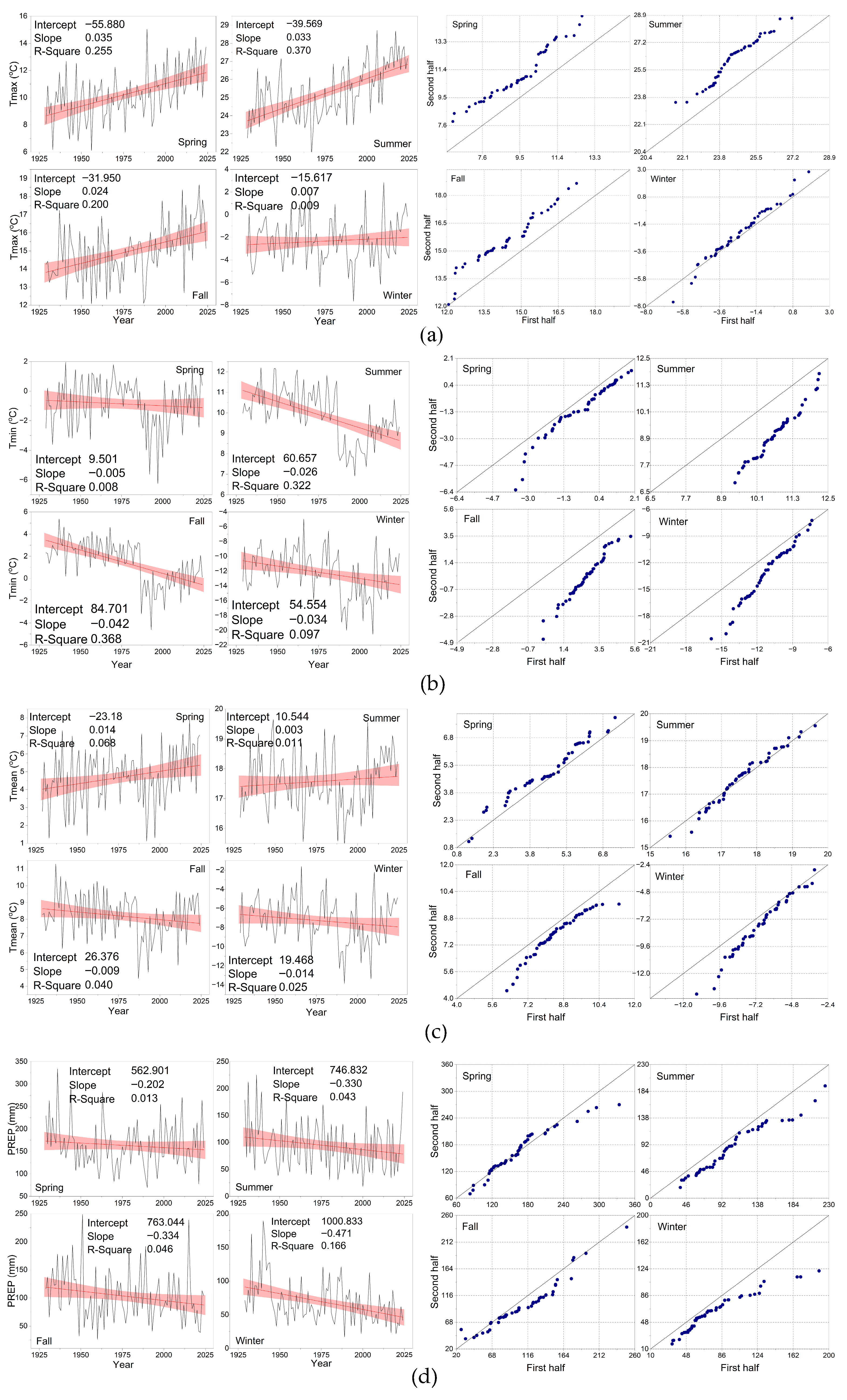
Figure 4 presents the seasonal trends (left column) and their ITA profiles (right column) for each of the climate variables considered, presented in groups of four. The trend graphs for the T_max time series (Figure 4a) in the left column show an upward trend in all seasons, parallel to the annual trend in Figure 3. However, the trend for the winter season is lower than for the others. In summer, the T_max series fits a line with a slope of 0.033 °C/year with a regression coefficient of R² = 0.344, while in winter it follows a line with a lower slope of 0.007 °C/year (R² = 0.009). In spring and autumn, the series fits to lines with slopes of 0.035 °C/year (R² = 0.255) and 0.024 °C/year (R² = 0.200), respectively.

The ITA profiles presented in the right column of Figure 4a, the MK test results in Table 1, and the results of Sen’s innovative approach in Table 2 support the view in the left column. According to the MK test, monthly average T_max values in spring, summer, and autumn exhibit an increasing trend at a significance level of 99%. 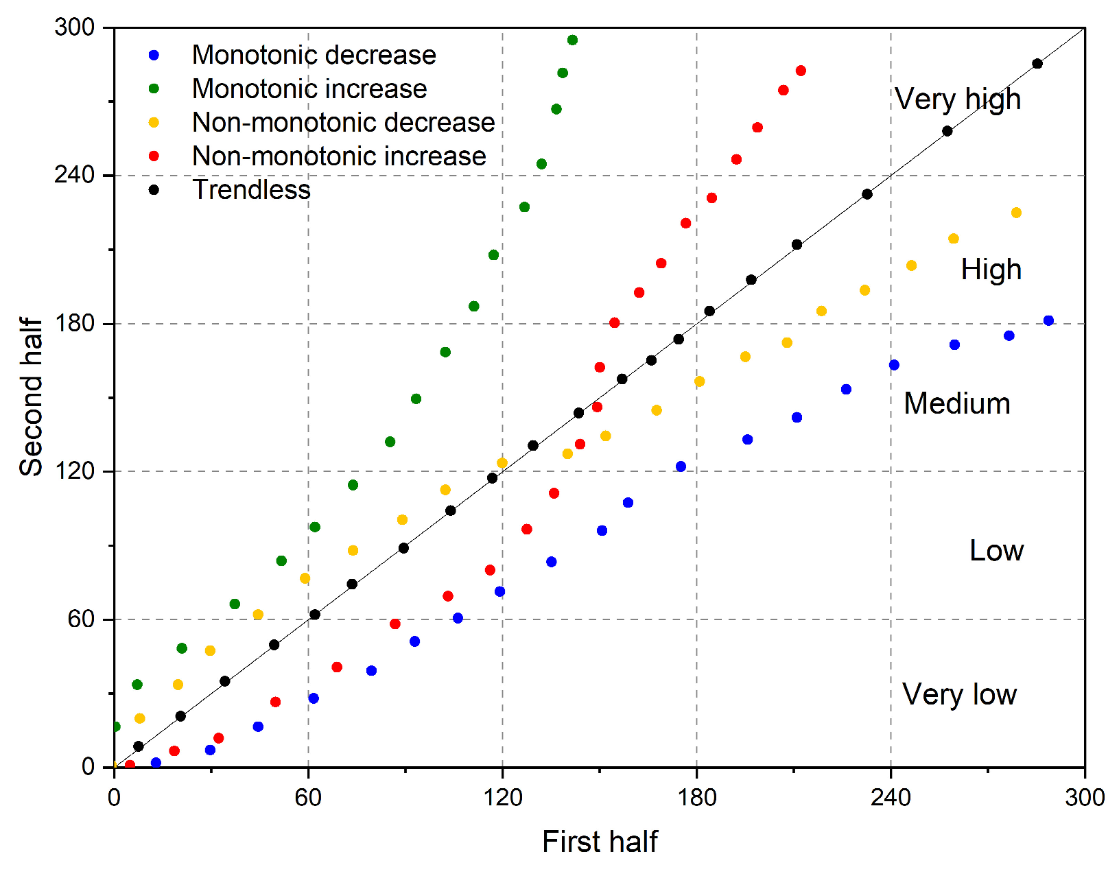The MK test Z statistics for spring, summer, and autumn have values of 4.81, 6.16, and 4.47, respectively, and are significantly greater than the critical z value of 2.575 (α = 0.01). According to the innovative trend analysis approach, there is no data in the “VL” category, which has low values in spring and summer, while there are monotonic increasing trends in the other categories of these seasons and in autumn. According to the MK test Z statistics for winter (0.95), no significant trend is observed, and the H₀ hypothesis is accepted. According to the ITA profile, winter exhibits a non-monotonic increasing trend, with higher values in the “H” and “VH” categories, although fewer values are present, showing an increasing trend.

Figure 4b shows the trend and ITA graphs for the T_min series. The trend of the time series for all seasons follows a direction parallel to the annual trend, and all ITA profiles are monotonically decreasing. The slopes of the linear fit lines for all seasons except spring are greater than or close to the slope of the annual linear fit line, which is −0.027 °C/year (R² = 0.225). The linear fit slopes of the seasonal trends in autumn and winter are −0.042 °C/year (R² = 0.368) and −0.034 °C/year (R² = 0.097), respectively, while this value is calculated as −0.005 °C/year (R² = 0.008) in spring. According to the MK test results in Table 1, the decreasing trend in the T_min series is statistically significant at the 95% significance level in winter and at the 99% significance level in summer and autumn. However, the trend in the T_min series in spring is not statistically significant at any of the selected significance levels (α = 0.1, α = 0.05, and α = 0.001), and the H₀ hypothesis cannot be rejected. Sen’s slope has values of −0.005, −0.023, −0.028, and −0.030 °C/year for spring, summer, autumn, and winter, respectively. There is no data in the “VH” category in autumn. Otherwise, there is a decreasing trend in all categories in all seasons. In spring, there is a large amount of data in the “H” and “VH” categories, where large values are present, while there is little data in the “VL” and “L” categories, where small values are present.

Figure 4c shows the trend and ITA plots for the T_mean series. The time series on the left show relatively increasing trends and positive slope values for spring and summer, while the opposite is true for autumn and winter. In the ITA scatter plots on the right, the autumn scatter plot exhibits a monotonic decreasing trend. A non-monotonic increasing trend can be observed in spring and summer, while the winter scatter plot resembles a non-monotonic decreasing trend. According to the MK test results summarized in Table 1, the spring T_mean series has a Z value of 2.45 (at an α = 0.05 significance level), indicating a significant increasing trend. In other seasons, the Ho hypothesis should be statistically accepted, and there is no trend for the T_mean. The annual MK test results for the T_mean series also revealed that there is no trend, and that the Ho hypothesis is accepted. The significant increasing trend calculated in the spring T_mean series is not valid for the T_mean series for the rest of the year.

According to the MK test, while no trend was determined in average temperatures in the annual analysis covering the period 1929–2024, seasonal analyses revealed an increasing trend in average temperatures in the spring at a 95% confidence level. When Sen’s slope values are examined in Table 2, it has a positive value (0.014, 0.005, and 0.007 °C/year) in spring, summer, and autumn, and a negative value (−0.012) in winter. This result may have been caused by the large dataset in the “VH” category in winter, i.e., the categories with the highest values. There are decreasing trends in the “VL” and “L” categories, i.e., the categories with smaller values, in spring, summer, and autumn. Consistent with the results of the MK test, there are increasing trends in the “VH” and “H” categories in spring.

One of the most striking results of the seasonal trend analyses of the selected climate variables was for monthly total precipitation. When the trend and ITA scatter plots of the PREP series shown in Figure 4d are examined, the time series are fitted with a linear slope with a negative value, parallel to the annual decreasing trend in all seasons. The ITA scatter plots show a non-monotonic decreasing trend in spring and autumn, while monotonic decreasing trends are observed in summer and winter. For the annual PREP series, the MK and ITA tests also determined decreasing trends. The MK test in Table 1 produced a Z statistic of −0.93 for the spring PREP series. According to the selected significance levels (α = 0.1, α = 0.05, and α = 0.001), this value is less than the critical z value, and therefore, the spring PREP series has no trend. According to the ITA results in Table 2, the Sen’s slope for the spring PREP series was calculated as −0.156. According to subcategorization, the spring PREP series exhibits a decreasing trend in the “VL” category, which has the lowest values, no trend in the “L” category, increasing in the “M” category, and decreasing in the “H” category. The MK test calculated decreasing trends for the summer, autumn, and winter PREP series at significance levels of α = 0.1, α = 0.05, and α = 0.001, respectively. According to the ITA approach, decreasing trends are also observed in different subcategories in summer, autumn, and winter.

One of the most striking results of the trend analyses of the PREP series, as explained above, is that important details can be revealed when trend analyses conducted on an annual scale are performed on a seasonal scale. Another important point is that the highest average precipitation in Erzurum between 1929 and 2024 occurred in spring, with 163.2 mm (Appendix A, Table A5). According to the trend analyses, there is no decrease in precipitation trends in spring.

During the study period, the lowest average precipitation in Erzurum occurred in winter, at 68.9 mm. According to MK tests, precipitation tends to decrease in winter at a 99% significance level. In cities where precipitation occurs primarily as snow during the winter season (January, February, and December), snow water may be the most significant potential recharger of groundwater resources, as opposed to rainwater runoff from asphalt and concrete pavements due to unplanned urbanization. Therefore, the decrease in winter precipitation trends is another important result of the trend analyses of the PREP series. A similar assessment can be made for the summer season. A decrease in precipitation trends during climatically dry summers (average 94.4 mm) is a potential factor that could increase the risk of drought.

3.3. Monthly Temperature and Precipitation Changes and Trend Analyses

Conducting temporal trend analyses of climate variables separately on annual, seasonal, and monthly scales provides more detailed information about the smaller time intervals of each variable. The MK test results indicate that increasing trends are statistically significant in the annual trend analyses of the T_max series. The ITA results also reveal monotonic increasing trends across all subcategories.

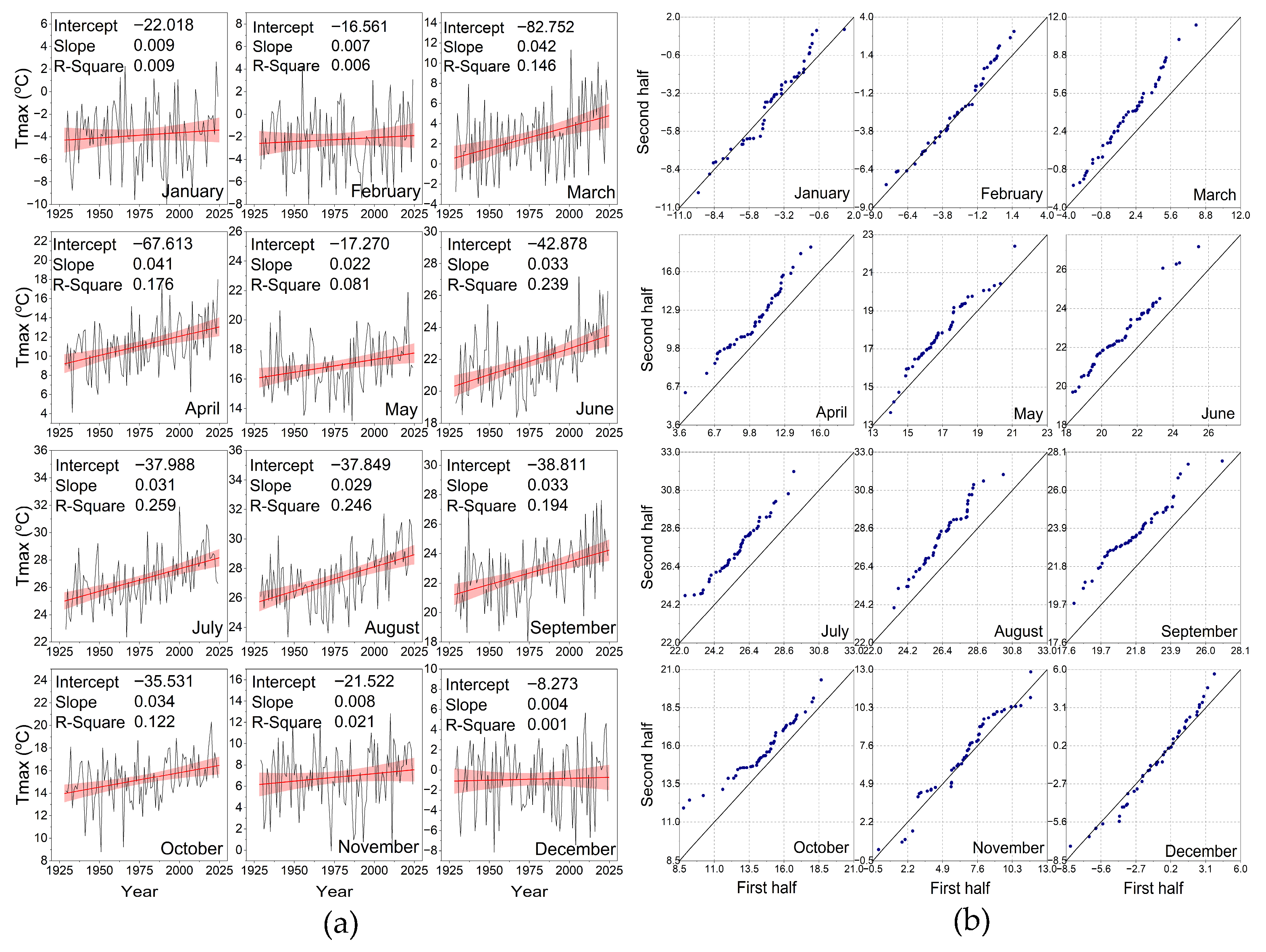
The MK test for seasonal trend analyses of the T_max series revealed no statistically significant trend in winter. Similarly, the ITA reveals increasing trends in the “H” and “VH” categories, where high values are found in winter, and decreasing or absent trends in other categories. The monthly trend analyses of the T_max series reveal monotonic increasing trends in March, April, June, July, August, September, and October, and nonmonotonic increasing trends in the other months (Figure 5b). According to the MK test results in Table 1, in line with the seasonal trend analysis, there are no statistically significant trends in the winter months (December, January, and February), nor in November. Increasing trends were calculated at a 95% significance level in October and 99% in other months. According to the ITA results in Table 2, increasing trends are observed in all categories in March, April, June, and August, and in the “H” and/or “VH” categories during the winter months. Figure 5b shows the high values in the “VH” categories of the ITA scatter plot for February, March, October, November, and December.

The monthly trend graph for the series in Figure 5a also shows relatively flat lines in November, December, January, and February, fitting the series. The fit line with the highest slope was 0.042 °C/year (R² = 0.146) for March, while the slope with the highest regression coefficient (R² = 0.259) was 0.031 °C/year for July.

Table 3. The results of the MK test show a seasonal decreasing trend (blue), increasing trend (red), and no trend (blank).

Tmax

Annual ***

Spring ***

Summer ***

Fall ***

Winter

M ***

A ***

M **

J ***

J ***

A ***

S ***

O **

N

D

J

F

Tmin

Annual ***

Spring

Summer ***

Fall ***

Winter **

M

A

M **

J ***

J ***

A ***

S ***

O ***

N ***

D **

J **

F **

Tmean

Annual

Spring **

Summer

Fall

Winter

M **

A **

M

J

J

A

S

O

N *

D

J

F

PREP

Annual **

Spring

Summer *

Fall **

Winter ***

M **

A

M

J **

J

A

S

O

N *

D

J **

F ***

* The significance level α = 0.10; ** The significance level α = 0.05; *** The significance level α = 0.01.

was created to provide a simpler representation of the analysis results, which exhibit a more complex pattern as the annual scale progresses from a monthly scale, compared to the MK test. It can be easily seen from Table 3 that the annual increasing trends for the temporal MK trend analyses described above for the T_max series become trendless in November and throughout the winter months as the temporal scale narrows.

Monthly trend and ITA scatter plots for the T_min series are given in Figure 6. The trend profiles (Figure 6a) show negative trends similar to the trend profiles of the annual and seasonal series except for March (slope = 0.008 °C/year; R² = 0.012). In Figure 6b, the ITA scatter profile of the March series shows a non-monotonic decreasing trend, but the strong increasing trend in the “VH” category may be the reason for the positive slope of the linear fit line in the trend profile. When the trend profiles are examined, the smallest linear fit slope was −0.007 °C/year (R² = 0.020) for the April series, while the highest slope was 0.051 °C/year (R² = 0.231) for the November series. Monotonic decreasing trends are observed in the ITA scatter plots for all months except January, February, and March. With the exception of the increasing trend (a small number of values) in the “VL” category of April, decreasing trends are observed for all categories of all months.

An examination of the MK test results in Table 1 reveals no statistically significant trend in the March and April series. Decreasing trends were calculated at a 95% significance level for the series in January, February, and December (winter months), and at a 99% significance level for the series in the remaining months. An examination of Table 3, which summarizes the MK trend test results for the T_min series across all time intervals, reveals that the T_min series exhibited no trend in the spring months, March, and April, while they exhibited a decreasing trend in all other time intervals. The maximum value of the MK test statistic, S (and Z), was calculated as −1549.0 (and −4.90) for September, rejecting the H₀ hypothesis and accepting the H₁ hypothesis.

The trend profiles and ITA scatter plots of the monthly mean temperature series are presented in Figure 7a,b, respectively. The linear fit lines of the time series for March, April, June, July, and August have positive slopes. The fit line with the highest slope was calculated for March at 0.028 °C/year (R² = 0.061). The fit lines of the T_mean series for the other months have negative slopes. The November fit line has the largest slope at −0.020 °C/year (R² = 0.039).

An examination of the ITA scatter plots of the T_mean series reveals monotonic increasing trends in April, nonmonotonic increasing trends in March and June, and monotonic decreasing trends in November. According to the ITA approach evaluation results presented in Table 2, the November scatter profile exhibits a decreasing trend in all subcategories, and the Sen’s slope is −0.016 °C/year. For March and April, the “VL” category, which contains the smallest data values, exhibits decreasing trends and no data, respectively, while the other subcategories exhibit increasing trends. The MK statistics in Table 1 also produce results supporting these trends. The H₀ hypothesis was rejected for March, April, and November. Despite the presence of increasing trends at the 95% level in March and April and decreasing trends at the 90% level in November, there is no statistically significant trend at the selected significance levels for all other months. According to the MK aggregate evaluation results for the T_mean series presented in Table 3, there are positive trends in the spring, March, and April, negative trends in November, and no trends in the other time periods.

The trend graphs and ITA scatter plots of the monthly total precipitation series are presented in Figure 8. When the trend profiles in Figure 8a are examined, the slope of the linear fit lines of the time series is negative in all months. The slope (and R²) values range between −0.218 mm/year (and R² = 0.132) and −0.035 mm/year (and R² = 0.001). The ITA scatter plots in Figure 8b show monotonic decreasing trends in January, February, March (with the exception of one data point above the 1:1 line), June, and September, nonmonotonic increasing trends in April, and nonmonotonic decreasing trends in the other months. Decreasing trends are observed in all categories of all months that exhibit monotonic trends, except for the “H” and “VH” categories of January and the “VH” categories of February and September, for which no data are available (Table 2).

During the 1919–2024 period, the highest average precipitation in Erzurum occurred in the form of rain in May (73.1 mm), April (54.6 mm), and June (48.5 mm). The lowest precipitation occurred in summer rain in August (17.6 mm) and snowfall in January (21.5 mm), December (22.0 mm), and February (25.4 mm). Precipitation statistics can be found in Table A5 of Appendix A. The May ITA scatter profiles show a trendless appearance until the decreasing trend in the “H” and “VH” categories, where the highest total precipitation values are found. In April, the ITA scatter profiles show a trendless appearance until the increasing trend in the “VH” category. Table 1 shows that, according to the MK test results, there is no statistically significant trend in the PREP series in either of these months, meaning that the Ho hypothesis is accepted. In Table 1, the ITA evaluation results for June show a Sen slope of −0.216 mm/year, and there are also decreasing trends in the “VL,” “L,” “M,” and “H” categories (no data in the “VH” category). The MK test also found a decreasing slope at the 95% significance level (Z = −0.210).

Apart from the increasing trends in the “VL” category in August and the “M” category in December (no data in the “VH” category), there are decreasing slope profiles in other subcategories. However, the MK test shows no statistically significant trend for these months, while decreasing trends are found in January and February at the 95% (Z = −2.62) and 99% (Z = −3.70) significance levels, respectively. According to the same results, November precipitation tends to decrease at the 90% (Z = −1.65) significance level.

When the monthly PREP series are evaluated with the results of the annual and seasonal series, it is seen that in winter, January and It is clear that February snowfall is showing a significant downward trend. While the decrease in total precipitation in November and June in the fall is significant enough to influence seasonal trends, the decreasing trend in March precipitation in the spring is not significant enough to significantly impact seasonal statistics (Table 3).

4. Discussion

This study conducted trend analysis using monthly data for maximum, minimum, and average temperature and total precipitation variables for Erzurum over a 96-year period spanning the period 1929–2024. The Erzurum Airport Station, whose data served as the basis for this study, was chosen because it provides the oldest meteorological records in the city. Undoubtedly, the results produced in the study do not define the large surface area of the city of 25,000 km². Daily average data from the station records were analyzed separately for each variable as annual, seasonal, and monthly time series. Analyses based on the MK trend analysis test and Sen’s ITA approach yielded significant findings.

A study conducted for western Iran, which is geographically close to the region covered in this study, identified increasing trends in the T_max series and decreasing trends in the precipitation series [56]. Similar trends for temperature and precipitation series were found in other studies conducted in Osijek, Croatia [57], and Serbia [7].

Increasing trends in the T_max series and decreasing trends in the T_min series were observed at strong statistical significance levels. Essentially, temperature differences between day and night are large in continental climate conditions. Changes in this variable, known as the diurnal temperature range (DTR), are important for determining the effects of climate change [58,59]. Due to the decreasing trend in T_min despite the increasing trend in T_max, DTR in Erzurum is increasing. Similar results have been found in studies examining DTR changes in Europe [60] and the continental United States [61]. The most important factors causing DTR oscillations are surface shortwave and longwave radiation [60]. Factors affecting these radiations include land use [62], irrigation, urbanization [63], desertification and other climate influences [63,64,65]. Investigating the underlying causes of DTR increases in this region could be a potential research topic.

Furthermore, there were no statistically significant trends in the T_mean series, apart from increasing trends for March and April. The trendless profiles observed in most of the average temperature series can be explained by the mathematical balancing of the increase in maximum temperatures and the decrease in minimum temperatures.

Trend analyses of the total precipitation series reveal strong decreasing trends in winter snowfall and in May, the month when Erzurum receives the most precipitation. Precipitation is the primary factor feeding the region’s groundwater and surface water resources, and these results in the precipitation series may increase the risk of drought in the region. In addition to the trendless appearance of the T_max and T_mean series in winter, the decreasing trends in the T_min and precipitation series indicate that the magnitude of the impact of temperature on the hydrological cycle requires further investigation [4]. The decrease in total precipitation trends could be due to changes in evaporation and relative humidity rates due to changing temperature dynamics, changes in land use, and/or increases in aerosol concentrations [66]. Each of these possible causes could be considered as potential research. In addition, investigating the relationship between ERA5 reanalysis data and temperature and precipitation variability by applying clustering techniques in the region with synoptic-scale circulation is also a potential study topic.