Abstract
Design storm hyetographs are essential inputs for hydrological modeling and flood risk assessment, yet their applicability in hyper-arid climates remains poorly constrained. In Saudi Arabia, engineers have frequently relied on imported synthetic profiles—such as such as the Natural Resources Conservation Service (NRCS; formerly the Soil Conservation Service, SCS) Type II curve—which were originally derived from temperate regions and may misrepresent the temporal structure of local storms. This study develops dimensionless design storm hyetographs for the southwestern provinces of Saudi Arabia (Asir, Al-Baha, Makkah, and Jazan) using a dataset of 8923 storms recorded at 152 rain gauges between 2017 and 2024. Storms were classified into four duration groups (<3 h, 3–6 h, 6–12 h, and 12–24 h), normalized by depth and duration, and analyzed through Huff quartiles, Euler Type II, Alternating Block Method (ABM), and NRCS Type II. Model–data evaluation using root-mean-square error (RMSE) identified Huff Q1 as the most representative profile for short and intermediate storms, while Huff Q2 best captured longer events. The optimized profiles consistently reproduced the strong front-loaded character of Saudi convective rainfall and outperformed existing synthetic hyetographs. These findings provide robust, locally calibrated design storms for flood modeling and infrastructure design in arid regions. The methodology is transferable to other data-scarce environments where standard profiles may misrepresent storm dynamics.
1. Introduction
Design storm hyetographs are essential for hydrologic design as they represent how rainfall intensity is distributed over time during extreme precipitation events [1]. In areas where historical records of severe storms are limited, synthetic hyetographs become indispensable for flood modeling and stormwater infrastructure planning [2]. Various methods for generating design storm profiles have been introduced in the literature, with the most common categories being geometric pattern approaches, frequency-based techniques, and data-driven methods [1,3]. Each of these methods reflects different assumptions and input requirements, and their selection can greatly influence the outcomes of hydrologic simulations.
Geometric pattern methods generate idealized storm shapes using simple geometric forms—such as rectangles or triangles—applied to a point on the intensity–duration–frequency (IDF) curve [4]. One widely used example is the Alternating Block Method (ABM), which arranges rainfall intensities in descending order around a central peak [4]. These methods are easy to apply and require limited data, making them useful in data-sparse regions. However, their symmetrical structure may fail to capture the true intra-storm variability observed in natural rainfall events, leading to inaccurate runoff predictions [3].
Frequency-based methods, like the Chicago hyetograph and Euler Type II pattern, utilize the full IDF curve corresponding to a particular return period to maintain statistical consistency in rainfall distribution [5]. These profiles typically feature a peak intensity located at a predetermined time fraction and arrange the remaining rainfall in a way that aligns with IDF sub-duration statistics [6]. Although these methods often result in more conservative runoff estimates by emphasizing early rainfall intensity, they can misrepresent actual storm dynamics, especially if the observed storm includes multiple peaks or delayed maximums [3,6,7].
In contrast, data-driven approaches rely on empirical storm records to derive dimensionless hyetographs that mirror actual rainfall behavior [8]. Huff’s quartile method is among the most recognized techniques in this category. It groups storms based on the timing of their peak rainfall and develops averaged cumulative rainfall curves for each class [8]. A conservative percentile, such as the 10%-exceedance curve of the first quartile, is often used in regions with convective storms to represent a worst-case scenario [2]. The principal advantage of this method lies in its reflection of real-world storm characteristics, but it demands a substantial volume of high-resolution rainfall data. In regions with sparse or inconsistent records, designers might resort to extrapolating extreme percentiles or supplementing empirical data with synthetic simulations [2].
Recently, clustering and machine learning approaches have been used to classify storm temporal patterns and to derive prototype hyetographs (e.g., k-means and DTW-based time-series clustering, as well as purpose-built hyetograph clustering such as HyetoClust). Improved separation among event types and efficient summarization have been reported when long, dense archives are available [9,10,11,12]. In the present study, Huff quartiles were selected as the principal empirical framework because interpretability, robustness under small/imbalanced samples, and regulatory familiarity were prioritized, and ABM, Euler, and NRCS/Type II were retained for benchmarking so that goodness-of-fit and engineering behavior could be judged on a common and transparent basis [13,14,15]. As denser regional records become available, clustering-based profiles can be evaluated side-by-side with Huff-based shapes using cross-validation on both statistical fit (e.g., RMSE) and hydrologic response metrics (e.g., peak-flow magnitude and timing).
Among widely adopted frameworks, the U.S. Soil Conservation Service (SCS)—now the NRCS—developed standard dimensionless hyetographs (Types I, IA, II, III) based on American storm datasets [16]. The SCS Type II profile is especially common in convective climates and features a symmetric distribution, with 50% of the rainfall centered in the middle third of a 24 h storm [16]. Its scalability and low data requirements have facilitated global adoption, particularly in regions with limited high-resolution records [17,18,19].
However, these standard profiles were originally tailored for temperate mid-latitude climates and may inadequately reflect the characteristics of storms in arid or tropical settings [2,16]. Several studies highlight the potential for design error when these generic profiles are applied in regions with fundamentally different meteorological dynamics. For instance, Al-Rawas and Valeo [7] documented that Omani convective storms are sharply front-loaded, diverging significantly from the gradual rise and fall modeled by the SCS Type II curve. Likewise, Awadallah and Younan [2] identified severe limitations when applying these curves in arid zones of the Middle East, cautioning that this practice can substantially underestimate flood risks.
Paradoxically, there are cases where standard hyetographs may be overly conservative. Kimoto et al. [6] analyzed monsoon events in semi-arid Arizona and noted that synthetic profiles tended to over-concentrate rainfall relative to observed records, thereby inflating flood predictions. This dual concern—of both under- and over-estimation—stresses the need for regional calibration to ensure reliable hydrologic design outcomes [3].
In the Middle East, and specifically in Saudi Arabia, the development of locally appropriate design storms is still maturing. Challenges such as insufficient data resolution, limited gauge coverage, and prior methodological errors have complicated past efforts. For example, both Al-Rawas and Valeo [7] and Elfeki et al. [18] encountered difficulties when processed rainfall data were mistakenly treated as raw time series, resulting in smoothed profiles that misrepresented peak intensities. This reinforces the importance of high-resolution and correctly interpreted data in the development of empirical hyetographs [7].
Despite these challenges, promising advances have emerged. In Oman, a detailed study of 236 storms from 17 gauges yielded hyetographs significantly different from standard SCS and UK patterns, with more pronounced early peaks [7]. Similar research in Qatar, Egypt, and Saudi Arabia has leveraged IDF curves and empirical techniques to propose storm distributions better aligned with local conditions [2]. Notably, Elfeki et al. [18] compiled a national dataset of 599 storm events across 28 stations, creating a set of regional and national dimensionless hyetographs. These curves often deviated from the SCS Type II profile, exhibiting front- or back-loaded patterns rather than symmetrical ones [18]. As a result, the authors recommended replacing imported hyetographs with Saudi specific versions in engineering applications.
Ewea et al. [20] extended this effort by applying Huff’s method to storm data from Makkah, constructing first- and second-quartile profiles for short and medium-duration storms. Their findings supported Elfeki’s earlier work: most Saudi storms peaked early, contrasting with the SCS assumption of a mid-storm peak. Likewise, Abdulrazzak et al. [16] demonstrated through hydrologic modeling in Medina that the SCS Type II pattern substantially under-predicted flood peaks compared to locally derived hyetographs. Their customized composite profiles, based on Medina storm records, yielded more accurate flood simulation results.
In the Al-Qassim region, Soliman [21] evaluated six design storm construction methods—including ABM, Euler, Huff quartiles, and existing Saudi and SCS profiles—using 557 storms from eight gauges. His analysis revealed wide variability among the methods, with the SCS Type II overestimating short-term intensities and Elfeki’s profile underestimating peak rainfall. Among the options, ABM-based hyetographs offered the best match to observed runoff, likely due to their ability to mimic front-loaded storm bursts typical in the region [21]. This finding reinforces the notion that no single global profile is universally suitable; performance depends heavily on local calibration and validation [3].
In summary, although substantial progress has been made in developing Saudi-specific design hyetographs, important gaps remain. Existing studies tend to be localized, focusing on a particular region or city (e.g., Makkah, Medina, Al-Qassim), and often rely on limited datasets [18]. Saudi Arabia’s diverse geography—ranging from humid coastal plains to hyper-arid deserts and mountainous zones—necessitates region-specific storm profiles rather than a national standard [16]. Moreover, the relative performance of various synthetic approaches under local conditions remains unresolved. While some international profiles might be adjustable for local use, others may require complete redevelopment. This issue is further compounded by ongoing data challenges, including sparse gauge coverage and limited sub-hourly rainfall records [2].
Addressing these limitations, the present study focuses on the southwestern region of Saudi Arabia, which is characterized by complex orographic effects and intense, short-duration convective storms. The region’s storm characteristics differ significantly from those of temperate zones where many standard hyetographs were developed. Recognizing the limitations of both foreign profiles and regionally constrained empirical curves, this study aims to develop a dimensionless hyetograph that accurately reflects the temporal distribution of rainfall in the southwest of Saudi Arabia. To achieve this, the study assesses the performance of widely used synthetic models—including SCS Type II, Huff quartiles, and Euler Type II—by comparing their temporal structures against observed storm events. Particular attention is given to each model’s ability to replicate peak rainfall timing and intensity distribution under arid conditions.
2. Materials and Methods
The study region encompasses the southwestern provinces of Saudi Arabia—Asir, Al-Baha, Makkah, and Jazan—bordered by the Red Sea to the west and the Arabian Desert (Najd/Rub’ al Khali) to the east. Elevations rise sharply from the coastal Tihamah plains (near sea level) to the Sarawat (Hejaz–Asir) Mountains, where Jabal Sawda (Asir) reaches nearly 3000 m above sea level [16]. This topographic gradient produces steep west-facing (windward) escarpments and more gradual east-facing (leeward) slopes.
Geologically, the region lies within the Arabian Shield and is deeply incised by wadis. Eastward, the terrain transitions to a broad plateau ranging from approximately 1600 to 2750 m, which gently slopes toward the Empty Quarter desert [22,23]. Along the Red Sea margin, the Tihamah coastal strip—typically 25–50 km wide—is hot and humid, with local relief reaching up to 400 m despite its designation as a “plain” [24].
Climatically, the region exhibits substantial variation. Most of the area falls under the hot-arid desert classification (Köppen BWh/BSh), while the higher elevations of the Sarawat Mountains experience a cooler, monsoon-influenced subtropical highland climate (Cwb) [25]. Orographic lifting of moist westerly air masses enhances condensation and precipitation along the windward slopes, particularly in the southern Hijaz ranges [23]. For example, the Asir highlands receive approximately 300 mm of rainfall annually, with nearly 60% occurring during the October–March Indian Ocean monsoon period [16,17,18]. In contrast, the lower coastal and interior plains receive only about 100 mm yr−1, primarily from sporadic convective storms [22,23,24,25].
Rainfall in the southwestern highlands is strongly seasonal. Spring (March–May) is typically the wettest period, contributing approximately 36.8% of the annual total [22,23]. Summer (June–August) also features substantial rainfall, with seasonal means reaching up to 205 mm due to intense convective monsoon storms [22]. Autumn (September–November) and winter (December–February) are comparatively drier, averaging around 160 mm and 114 mm, respectively. Winter precipitation is generally associated with cyclonic systems and tends to be less intense than summer convection [22].
Spatial variability in rainfall is pronounced across the region. The wettest belt lies along the upper windward escarpments of the Asir and Al-Baha mountains, where annual totals can approach 580 mm [26,27]. Immediately east of the crest, a marked rain shadow effect reduces precipitation to approximately 115–190 mm yr−1, while the Red Sea coastal plain exhibits similarly low rainfall, averaging around 115 mm yr−1. Rainfall intensity and frequency tend to decrease northward along the coast [28,29].
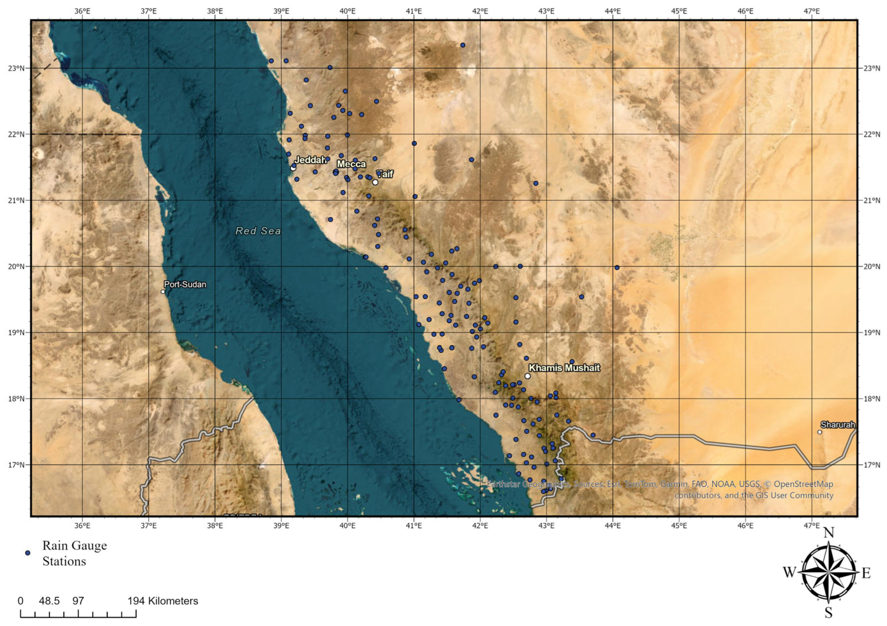
To monitor this variability, the Ministry of Environment, Water and Agriculture (MEWA), Riyadh, Saudi Arabia, maintains a network of 151 rain gauge stations distributed across southwestern provinces. These stations (blue dots in Figure 1) provide critical data for hydrological modeling, climatological analysis, and water resource management in a region where precipitation is both spatially heterogeneous and seasonally concentrated. Spatial coverage and station density were noted to be uneven across complex orography, so representativeness may be reduced in sparsely instrumented sub-regions: this limitation was considered when interpreting duration-class frequencies and temporal patterns.
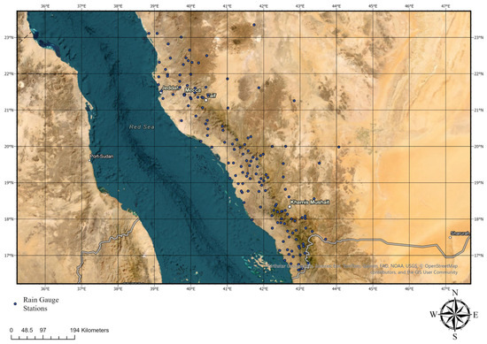
Figure 1.
Location of the study area in southwestern Saudi Arabia (Asir, Makkah, Al-Baha, and Jazan) and distribution of the 151 MEWA rain gauges.
3. Methodology
Rainfall time series from 152 gauges across Saudi Arabia were compiled by MEWA for the period 2017–2024. The data was quality-controlled to remove duplicates and erroneous values, while missing entries were retained for transparency. Storm events were identified using an inter-event dry period (IDP) was set to 6 h, following hydrologic convention that shorter quiescent periods represent the same convective event, whereby a new event begins after a continuous zero-rainfall interval exceeding the IDP [30].
To ensure hydrological relevance, segmented events were filtered using predefined minimum depth and duration criteria.
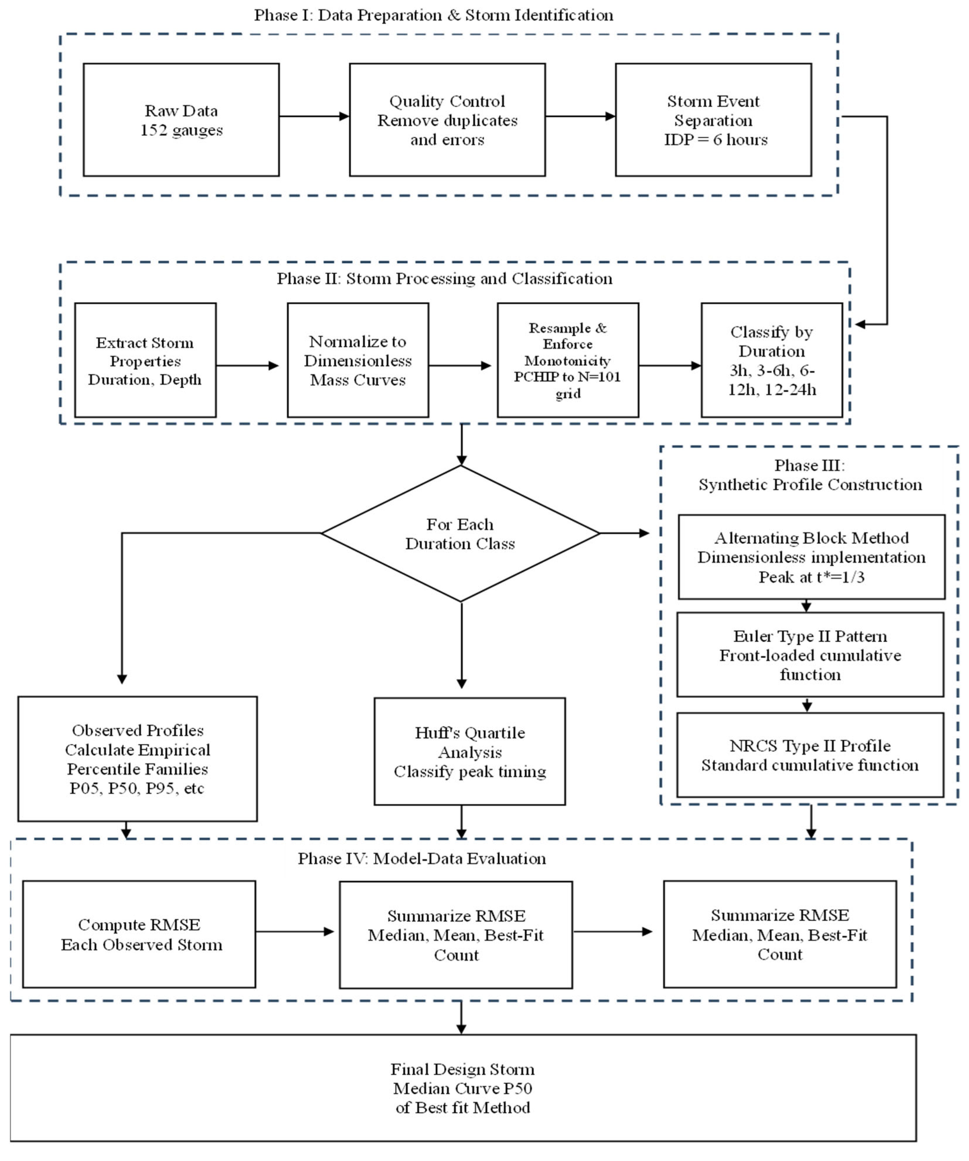
A step-by-step workflow is summarized in Figure 2. The sequence is: (i) data acquisition and QC; (ii) event identification (IDP = 6 h) and hydrologic filters; (iii) conversion of each event to a dimensionless mass curve so shapes can be compared independent of duration and depth; (iv) duration-class stratification; (v) Huff quartile assignment; (vi) construction of candidate dimensionless profiles (Huff, ABM, Euler Type II, NRCS/Type II); (vii) goodness-of-fit evaluation and selection of a design curve for each duration class.
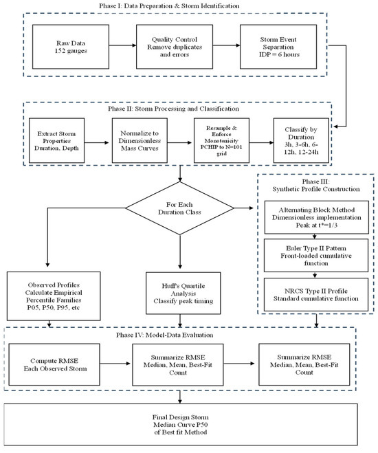
Figure 2.
Flowchart showing the applied methodology.
For each identified storm, start and end times, total duration in minute, total depth in mm, and incremental depths were preserved for subsequent processing. Each storm was converted to a dimensionless mass curve to enable shape-based comparisons independent of absolute duration and depth. Time and cumulative depth were normalized as
Monotonicity was enforced by accumulating non-negative intensities; if needed, minor numerical artifacts were corrected by isotonic regression applied to the cumulative series only. All curves were resampled on a common grid of points over using monotone piecewise-cubic interpolation (PCHIP).
To ensure a balance between representativeness and sample size, storm events were classified into four duration-based categories: less than 3 h, 3–6 h, 6–12 h, and 12–24 h. These categories were applied consistently throughout the profile construction and comparative analyses.
Huff’s quartile analysis was applied to classify storms according to the timing of their peak intensity. The method divided each storm duration into four equal quartiles. The peak rainfall was identified, and the storm was assigned to a quartile based on the position of the peak.
where is the total storm duration and is the time of maximum rainfall.
For each duration class, a suite of candidate dimensionless design storm profiles was constructed and subsequently evaluated alongside the observed percentile envelopes derived from the normalized storms. First, the observed ensembles were summarized as empirical percentile families together with the median curve . These curves provide a data-driven dimensionless cumulative function, denoted , that characterizes the central tendency and spread of storm temporal patterns in each class.
The Alternating Block Method was implemented on a dimensionless basis without invoking a regional IDF. A monotone reference cumulative depth function with unit total depth was evaluated at nested sub-durations . Incremental blocks were then computed as
The set as sorted in descending order and placed alternately about a prescribed peak-time fraction (center-peaked), after which the sequence was integrated to yield the cumulative hyetograph and normalized to obtain the ABM dimensionless curve .
A Euler Type II pattern was also constructed as a front-loaded dimensionless cumulative function specified to accumulate approximately 40% of the depth by one-quarter of the duration and to peak near
Also, NRCS (formerly SCS) Type II distribution was applied via its dimensionless cumulation . In all cases, the candidate profiles were represented on the common normalized time grid as dimensionless cumulative curves to enable direct, like-for-like comparison with the observed ensembles during subsequent model–data evaluation.
All curves (observed and each candidate ) were resampled on the common grid of over . For each storm and method, the root-mean-square error (RMSE) was computed as
Within each duration class, RMSE was summarized per method by the median (primary) and mean (secondary), and the best fits count was recorded (number of storms for which a method achieved the lowest RMSE). The class best fit was selected primarily by the smallest median RMSE, with the best fits used as a tie-breaker.
For each duration class, the design storm mass curve was defined as the median () dimensionless curve of the winning method. Where required for sensitivity analysis, lower/upper envelopes () were also retained.
4. Results
The analysis of storm duration was undertaken as the first step toward developing the design of storm hyetographs. Across 152 gauges for the period 2017–2024, a total of 8923 storm events were identified, with individual durations ranging from approximately 10 min to 24 h. To characterize the distribution, a frequency histogram was constructed using 3 h bins (0–3, 3–6, 6–9, 9–12, 12–15, 15–18, 18–21, and 21–24 h). The resulting distribution is presented in Figure 3. In the figure, bars depict the relative frequency (%) for each bin and value labels provide the exact percentages.
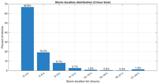
Figure 3.
Storm duration frequency histogram (3 h bins) for the combined dataset (n = 8923; 2017–2024; 152 gauges). Bars indicate the percentage of storms in each bin; value labels show exact percentages.
From the histogram, a pronounced right-skewed pattern was observed. The largest share of storms was found in the first bin (≤3 h), which accounted for 66.805% of all events (n = 5961). The second bin (3–6 h) contributed 19.153% (n = 1709). Bins beyond 6 h were sparsely populated when treated individually; collectively, durations between 6 and 24 h represented 14.042% of events (n = 1253), distributed across the 6–9, 9–12, 12–15, 15–18, 18–21, and 21–24 h bins. This concentration of events in the shorter durations is consistent with convective storm behavior in arid to semi-arid climates and indicates that short, intense events dominate the record.
For subsequent analyses that require adequate sample sizes per class (e.g., percentile-based profile development and comparative hyetograph construction), durations were consolidated into four groups: <3 h, 3–6 h, 6–12 h, and 12–24 h. The resulting counts and relative frequencies are summarized in Table 1. By design, the first two groups span 3 h each, the third group spans 6 h, and the fourth group spans 12 h. This grouping strategy was adopted to balance representativeness (dominant short-duration storms) with statistical stability in the longer-duration classes.

Table 1.
Storm-duration groups, sample sizes, and relative frequencies used in subsequent analyses.
The results in Figure 3 and Table 1 collectively indicate that more than two-thirds of all detected storms were short-duration events (≤3 h), with approximately one-fifth occurring over 3–6 h. Only about one-seventh of events extended beyond 6 h. These findings justify the adoption of the four-group scheme and provide the basis for developing duration-stratified design storm hyetographs in subsequent sections.
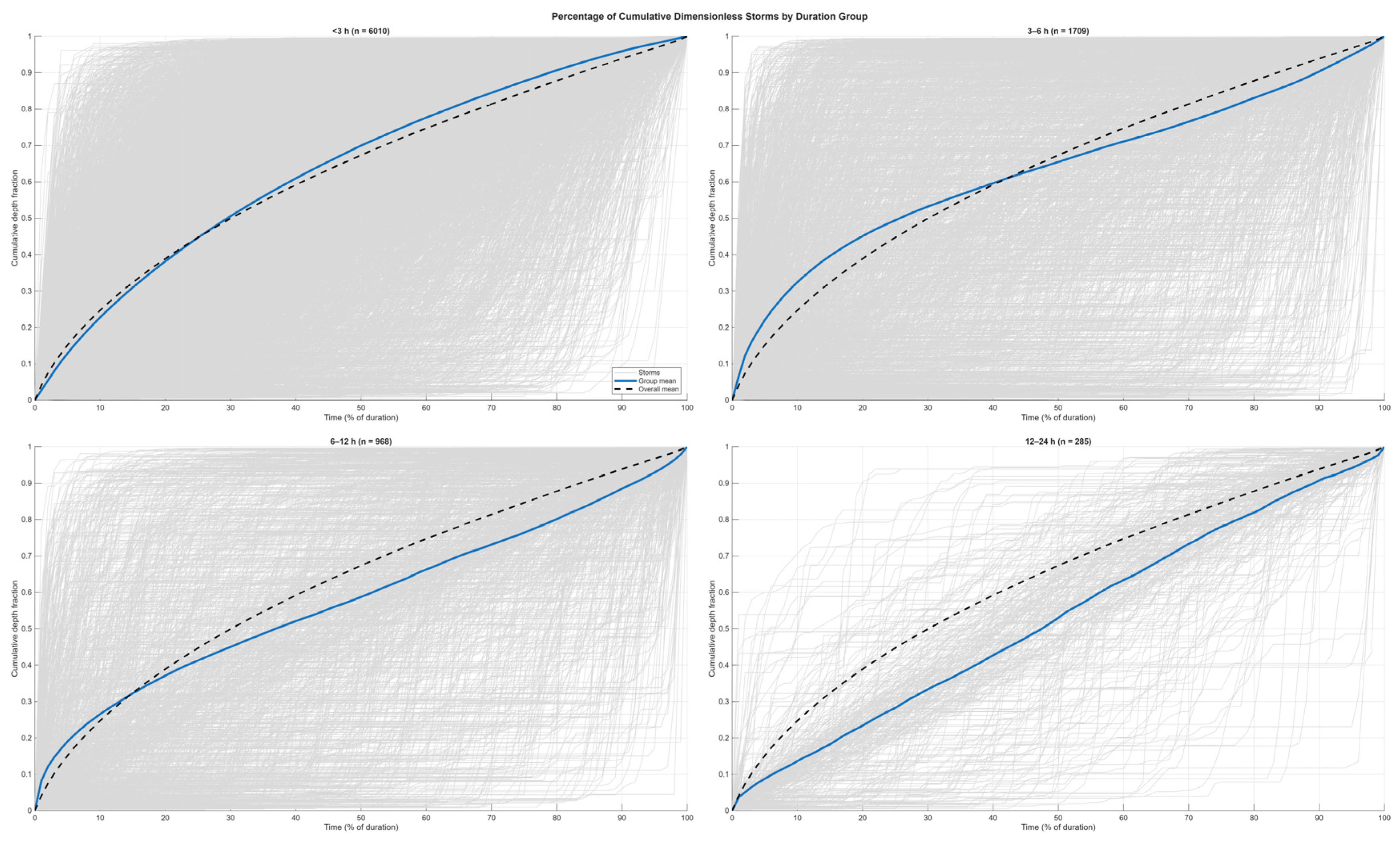
Storms were partitioned into the four duration classes defined in Table 1 (<3 h, 3–6 h, 6–12 h, and 12–24 h). For each class, Figure 4 presents all dimensionless cumulative rainfall curves (gray), the corresponding class-mean curve (colored solid), and the overall mean across all storms (black dashed). The groups therefore summarize, within each duration range, how rainfall accumulated as a fraction of total depth over the normalized storm time (0–100%).
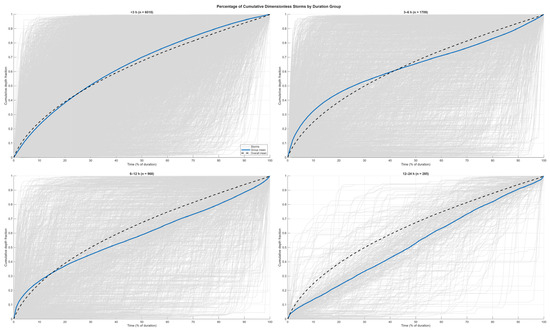
Figure 4.
Dimensionless Temporal Distribution by Duration of the group, Gray polylines show the cumulative depth fraction of every individual storm in the class; the colored solid curve shows the class (duration-group) mean; the black dashed curve shows the overall mean across all storms (pooled over classes). Panel titles give the duration class and sample size . Time on the x-axis is expressed as % of event duration (0–100%), and the y-axis is the cumulative depth fraction normalized to unit total depth.
In the <3 h class, a strongly front-loaded temporal pattern was observed. The class-mean curve rose steeply within the earliest portion of the duration and remained above the overall mean through the first half of the event. The dense band of gray traces near the upper envelope at early times indicates that many short storms contributed a substantial fraction of their depth shortly after onset. The spread of individual curves within this class was comparatively narrow relative to the longer classes, reflecting a more consistent temporal structure among short events.
In the 3–6 h class, early accumulation persisted but with reduced concavity compared with the <3 h group. The class-mean curve tracked slightly above, or close to, the overall mean until mid-durations and then converged toward it. The ensemble of individual curves exhibited greater dispersion than in the <3 h class, indicating increased variability in how rainfall was distributed within storms of intermediate short duration.
In the 6–12 h class, a more gradual onset of accumulation was evident. The class-mean curve lay below the overall mean during the first half of the normalized duration and approached it later in the event, which indicates that a larger share of the total depth was delivered in the mid- to late portion of these storms. The scatter of individual traces increased further, showing a broader range of within-storm timing among longer events.
In the 12–24 h class, the class-mean curve approached an approximately linear increase with time and remained near the one-to-one diagonal for much of the duration. This pattern indicates a comparatively uniform cumulative rise over long events. The widest spread among individual curves was also observed in this class, which is consistent with the wider variety of meteorological conditions that can produce day-scale storms and with the smaller sample size noted in Table 1.
Across the four groups, systematic differences among the class-mean curves were apparent. The overall mean (black dashed) lay closer to the means of the two shorter-duration classes during the early portion of the duration and exhibited greater separation from the 6–12 h and 12–24 h means in the first half of the event, a pattern that reflects the dominance of short storms in the sample (Table 1). Figure 4 therefore provides a duration-stratified empirical basis for subsequent development and evaluation of design hyetographs without inferring mechanisms or implications beyond the observed shapes.
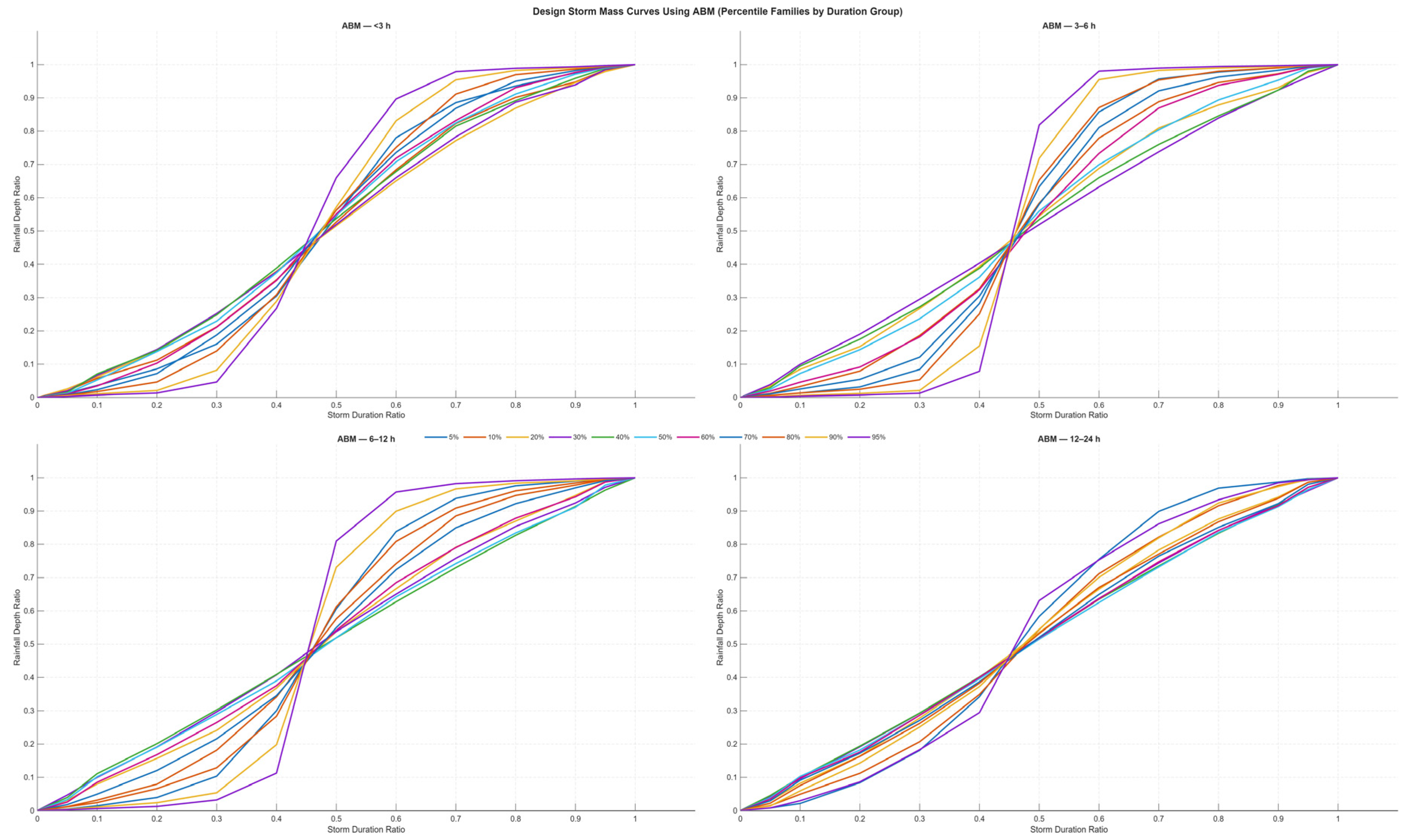
Figure 5 presents the design storm mass curves derived with the ABM for the four duration groups (<3 h, 3–6 h, 6–12 h, and 12–24 h). The curves are shown as cumulative rainfall depth ratios plotted against the storm duration ratio, with percentile families from 5% to 95%.
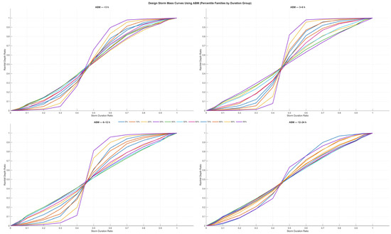
Figure 5.
Design storm mass curves using the Alternating Block Method (ABM) for each storm duration group.
For the <3 h group, all percentile curves originate at zero and reach unity at the end of the duration axis. A rapid rise is observed near the mid-portion of the storm, after which the curves gradually approach their final value. The separation among percentiles is most apparent in the middle half of the duration, where the 90–95% curves rise earlier and the 5–20% curves rise later, while the 40–60% curves plot centrally between these bounds.
For the 3–6 h group, a pronounced increase in cumulative depth occurs around the middle of the storm duration. The 90–95% percentile curves exhibit the steepest mid-segment transition, whereas the lower percentiles (5–20%) show a delayed increase. Despite this spread, all curves converge smoothly to unity near the end of the duration axis.
In the 6–12 h group, the cumulative curves show a more gradual ascent in the early portion (up to approximately the first half of the duration) followed by a steady rise toward the end of the storm. The spacing among percentiles is visible across the entire duration, with the interpercentile band relatively consistent from the first third through the final third of the curves.
For the 12–24 h group, the percentile family appears smoother across the duration. The cumulative curves increase steadily from start to end with comparatively modest separation between adjacent percentiles. As with the other groups, all curves start at zero and reach unity at the completion of the duration axis.
Across all groups in Figure 5, the percentile families demonstrate the expected monotonic behavior of cumulative mass curves, beginning at zero rainfall depth ratio, increasing without decline, and approaching a normalized value of one by the end of storm duration. Differences among groups are reflected in the steepness and spread of the percentile families along the duration axis.
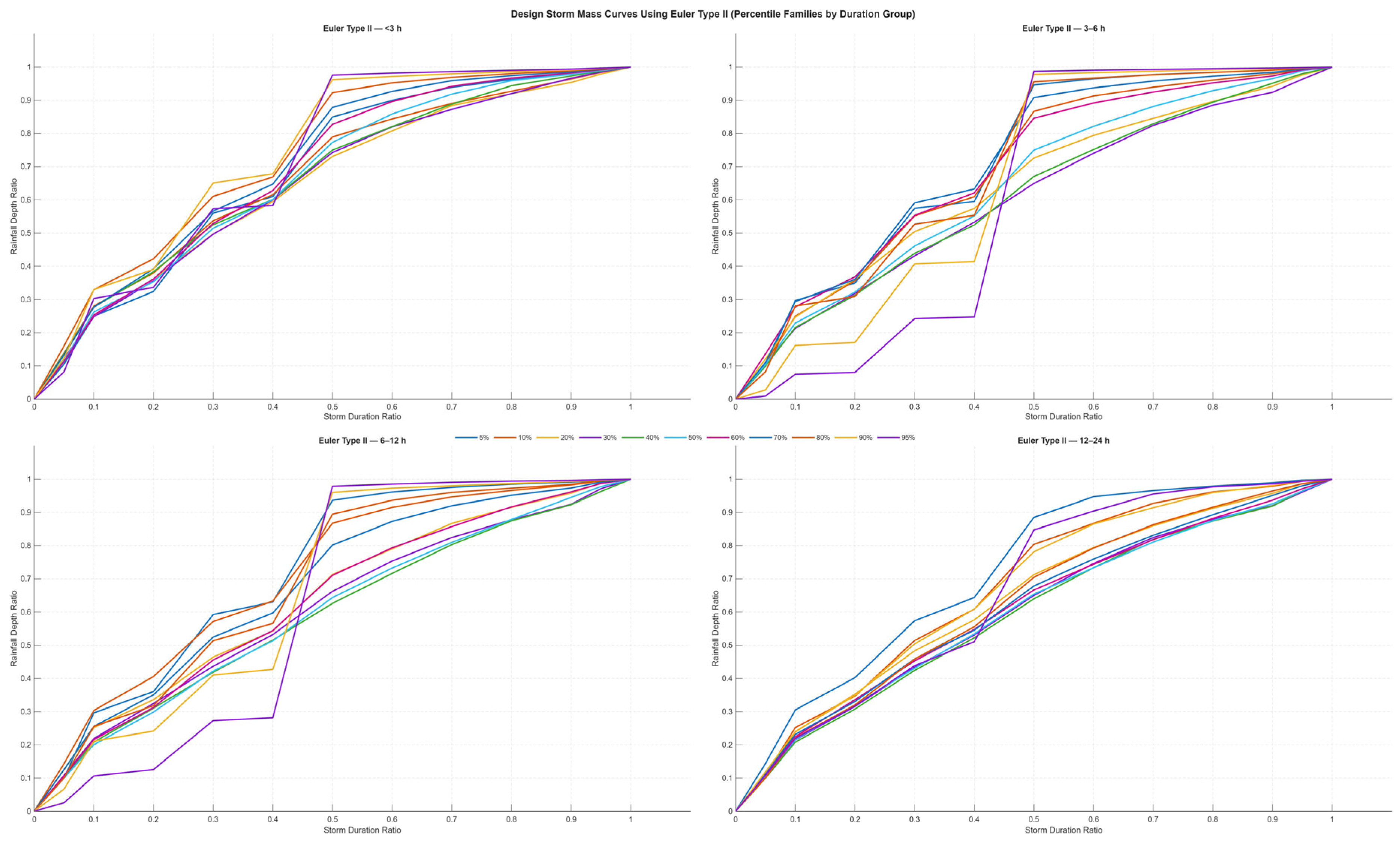
Figure 6 displays the design storm mass curves produced using the Euler Type II arrangement for the same four duration groups, again shown as percentile families from 5% to 95% on rainfall depth ratio versus storm duration ratio axes.
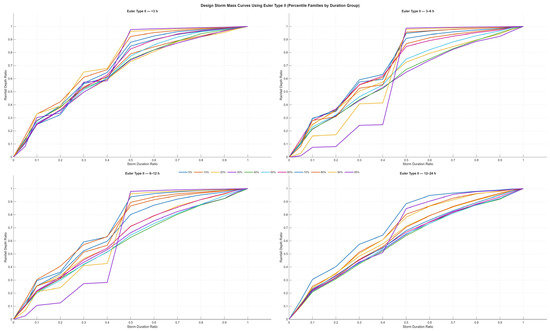
Figure 6.
Huff percentile design storm mass curves (P05–P95).
In the <3 h group, the percentile curves indicate a relatively rapid accumulation over the early to middle portion of the storm. The higher percentiles (90–95%) rise earlier and reach higher cumulative ratios sooner than the lower percentiles, while all curves converge to unity at the end of the duration.
For the 3–6 h group, the percentile family shows a distinct steepening between approximately one-third and one-half of the duration, after which the curves flatten as they approach unity. The spread among percentiles is apparent throughout this midsegment, with the 50% curve centrally positioned between lower and higher percentile bounds.
In the 6–12 h group, the cumulative profiles increase gradually in the first portion of the duration and then accelerate through the middle segment before tapering toward the end. Separation among percentiles persists across the duration, with noticeable clustering of the mi percentiles around the central part of the curve.
For the 12–24 h group, the percentile curves rise more evenly over the storm duration. The family of curves remains closely grouped compared with shorter duration groups, and all curves terminate at a rainfall depth ratio of one.
Overall, Figure 6 shows that, for each duration group, the cumulative rainfall depth ratio increases monotonically with storm duration ratio and that the ordered set of percentile curves provides a consistent envelope from lower (5–20%) to higher (90–95%) percentiles. The families begin at zero, show a progressive rise, and reach unity at the end of the normalized duration axis for all groups.
Across all duration classes, the location of the peak incremental intensity was most frequently identified in Quartile 1 (Q1) (0–25% of the storm duration). In the <3 h group (n = 5961), counts by quartile were 3348, 1425, 796, and 392 for Q1–Q4, corresponding to 56.2%, 23.9%, 13.4%, and 6.6%, respectively. In the 3–6 h group (n = 1709), the distribution was 1011, 216, 213, and 269 (59.2%, 12.6%, 12.5%, 15.7%). For 6–12 h events (n = 968), counts were 503, 154, 135, and 176 (52.0%, 15.9%, 14.0%, 18.2%). In the 12–24 h class (n = 285), counts were 89, 77, 78, and 41 (31.2%, 27.0%, 27.4%, 14.4%) (Table 2).

Table 2.
Number of Storms for Each Quartile (by Duration Group).
When aggregated over all storms (n = 8923), the totals by quartile were 4951 (Q1), 1872 (Q2), 1222 (Q3), and 878 (Q4), which represent 55.5%, 21.0%, 13.7%, and 9.8% of the sample, respectively. Thus, the peak most commonly occurred in the first quarter of the storm duration, while later-quartile peaks were less frequent.
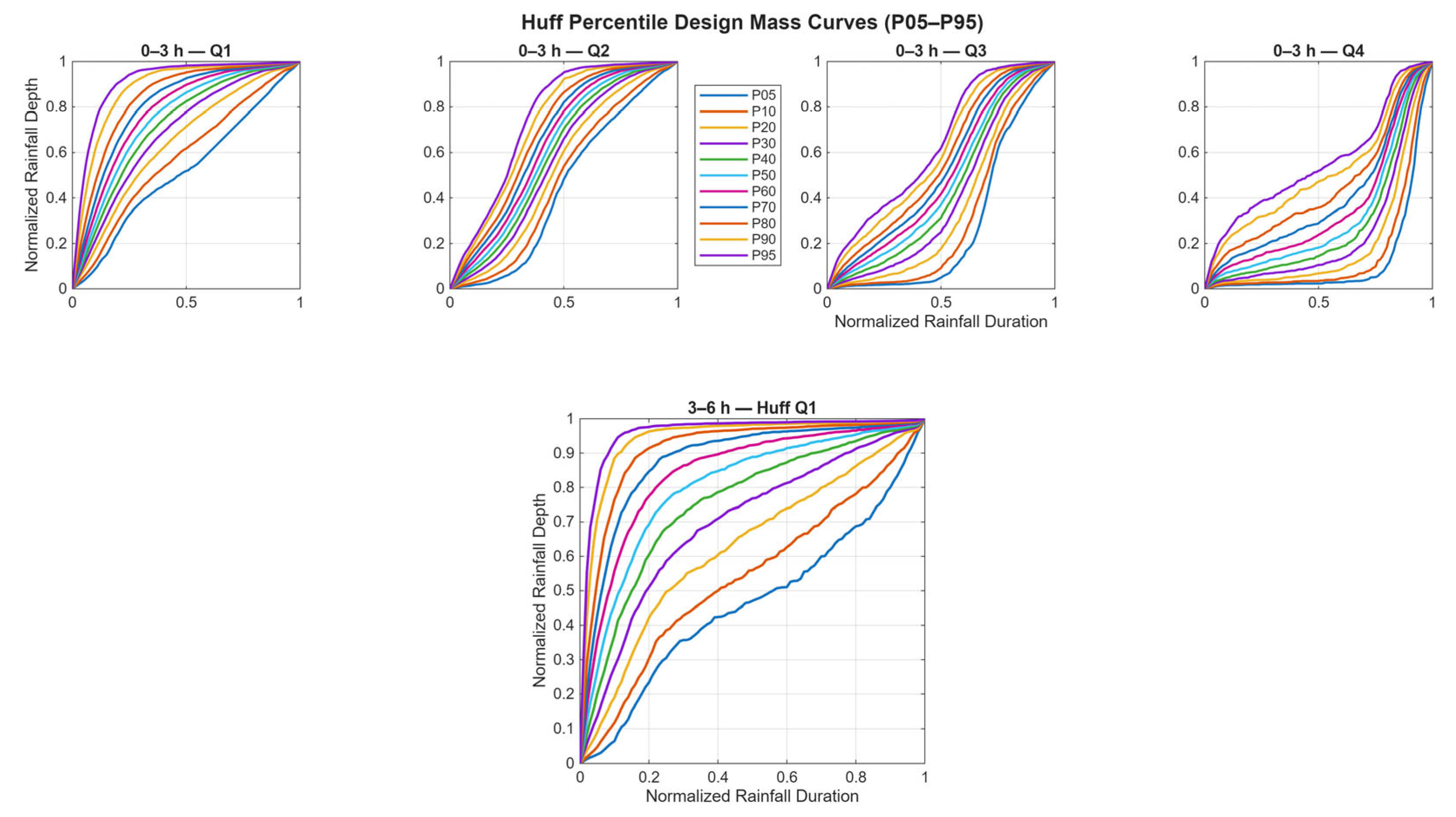
Figure 7 presents percentile families (P05–P95) of cumulative rainfall depth ratio versus storm duration ratio constructed with the Euler Type II arrangement for each duration class. For the <3 h group, the curves rise rapidly between approximately the first third and one-half of the normalized duration, with higher percentiles (≥P90) attaining larger cumulative ratios earlier than lower percentiles, and all curves converging to unity at the end of the duration axis. In the 3–6 h group, a similar pattern is shown: a pronounced steepening around the early-to-mid portion of the storm, followed by a gradual approach to the terminal value; the percentile spread is most visible in this midsegment.
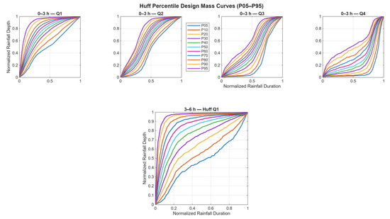
Figure 7.
Huff Percentile Design Storm Mass Curves for Group 1 (0–3 h, Q1–Q4) and Group 2 (3–6 h, Q1).
In the 6–12 h group, the percentile curves increase more gradually at the start, then exhibit an acceleration around the middle portion of the duration before tapering toward the end; separation among percentiles persists across the entire curve, with the median (P50) positioned centrally between the lower and upper envelopes. The 12–24 h group shows smoother, more evenly increasing cumulative profiles across percentiles, with a relatively tight family of curves and a steady rise from zero to one over the full normalized duration.
Across all four groups in Figure 7, monotonic behavior is maintained, and the ordered percentile families provide consistent envelopes from lower (P05–P20) to higher (P90–P95) curves, illustrating the range of cumulative mass distributions observed within each duration group under the Euler Type II arrangement.
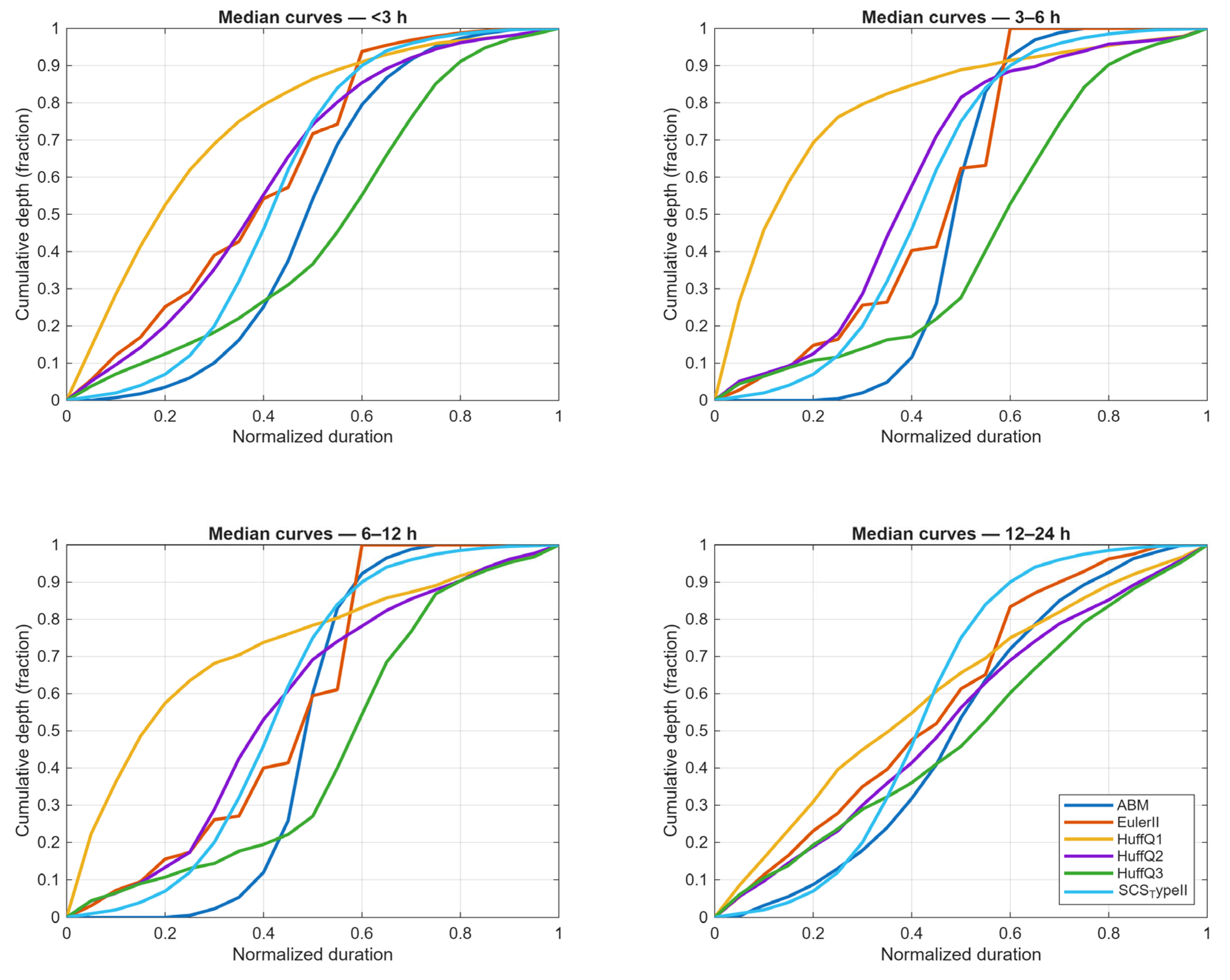
The median cumulative depth curves for the six methods (ABM, Euler Type II, Huff Q1, Huff Q2, Huff Q3, and SCS Type II) are displayed for the four duration classes in Figure 8. In the <3 h group (n = 5961), the Huff Q1 and Huff Q2 medians rise most rapidly during the early part of the normalized duration, whereas the Huff Q3 median exhibits a later rise; ABM shows a near-symmetric S-shape and the SCS Type II curve is strongly front-loaded. In the 3–6 h group (n = 1709), the family of medians remains ordered and monotonic; the Huff Q1 median lies above the others through the first half of the duration, while Huff Q3 again concentrates later. In the 6–12 h group (n = 968), the medians become less front-loaded overall; Huff Q2 and Huff Q1 align with the middle of the envelope and Huff Q3 maintains a comparatively later rise. In the 12–24 h group (n = 285), the median curves are smoother and more evenly distributed across the duration; Huff Q2–Q3 occupy the central envelope while SCS Type II remains earlier rising than most other medians.
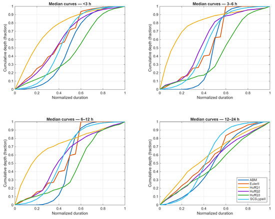
Figure 8.
Median (50th-percentile) design storm cumulative curves by duration group and method.
Goodness-of-fit was evaluated between each observed storm and the six median profiles by computing the root mean square error (RMSE) on a normalized-time grid at 5% increments. For each storm, the profile yielding the lowest RMSE was identified as the best fit. Summary statistics for these results are provided in Table 3.

Table 3.
RMSE Statistics and Best-Fit Counts by Method and Duration Group.
Goodness-of-fit results, summarized in Table 3, show that the Huff quartiles outperform the purely synthetic profiles, with a clear duration-dependent pattern: Huff Q1 best matches short-duration storms (<3 h and 3–6 h) and remains competitive in 6–12 h, whereas Huff Q2 is preferred for 12–24 h events. This transition indicates front-loaded accumulation at short durations and more even accumulation for day-scale storms. The relatively poorer fits of NRCS Type II and Euler Type II reflect mid-peaking timing that does not align with the early rise in the regional record, while ABM’s spikier structure yields higher error against the observed central tendency. Table 3 reports the mean/median RMSE values and the per-storm best-fit counts that underpin these statements.
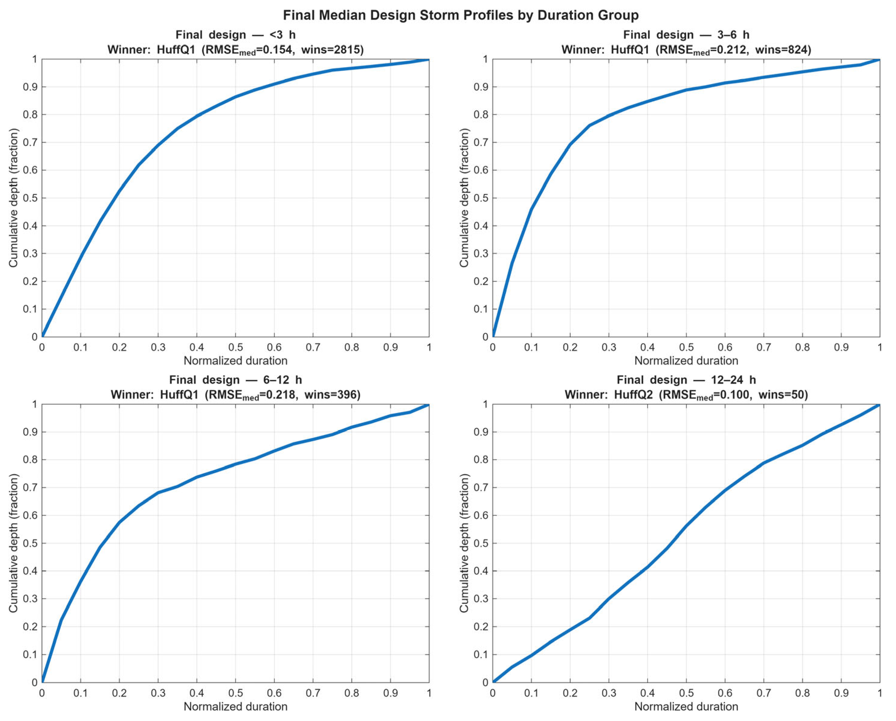
For design and modeling, Huff Q1 is an appropriate baseline shape for durations < 12 h, capturing early intensity that governs peak discharge, whereas Huff Q2 is more suitable for 12–24 h where accumulation is more even. Using mid-peaking distributions would tend to delay the intensity peak and underestimate early peaks in runoff simulations, whereas adopting ABM by default may over-emphasize spikes relative to typical storms. The selected profiles in Figure 9 provide duration-stratified, region-calibrated shapes, and the dimensionless coordinates for each selected profile are given in Table 3 for direct implementation.
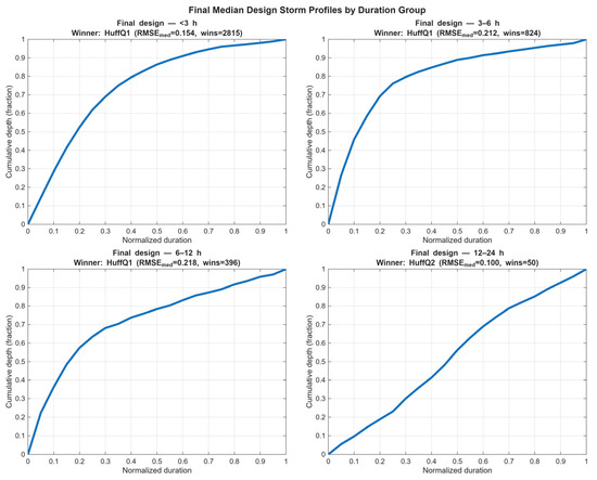
Figure 9.
Final median design storm profiles by duration each group.
The final design profiles selected by the objective rule are presented in Figure 8. Consistent with the goodness-of-fit patterns, the selected profiles in Figure 8 show a transition from a strongly early-rising shape at short durations (<12 h; Huff Q1) to a more even accumulation at long duration (12–24 h; Huff Q2), with a smooth approach to unity near the end of the event.
Across groups the shape transitions from strongly early rising at short durations to more evenly distributed accumulation at long durations.
Table 3 provides the dimensionless storm mass curves for the four duration classes as numerical pairs of normalized time (τ; 0 to 1 at 5% increments) and cumulative depth fraction F(τ). Each column corresponds to a duration group and contains the coordinates of the best fit profile shown in Figure 9 (Huff Q1 for <3 h, 3–6 h, and 6–12 h; Huff Q2 for 12–24 h). The table thus supplies a ready-to-use design mass curve for each class without further transformation.
Table 4 reports the selected (best-fit) dimensionless design storm mass curves for each duration class, tabulated as pairs of normalized time τ (0–1 at 0.05 steps) and cumulative depth fraction F(τ). Inspection shows that in the early portion (τ ≈ 0.05–0.30), the <3 h and 3–6 h profiles exhibit the largest F(τ), indicating front-loaded accumulation in short events. At intermediate times (τ ≈ 0.40–0.70), the 6–12 h profile rises more steadily than the shorter-duration classes, reflecting reduced front-loading. In the late portion (τ ≥ 0.70), the 12–24 h profile approaches unity smoothly and near-linearly, consistent with a more even temporal distribution. Because coordinates are given at uniform 5% increments, Table 4 can be used directly to synthesize design hyetographs and to couple the dimensionless mass curves with site-specific IDF inputs in subsequent applications.

Table 4.
Best-Fit Dimensionless Design Storm Mass Curves by Duration Class.
5. Discussion
This result is consistent with prior findings that empirical arid-region storms tend to be front-loaded, whereas the Type II curve peaks in the middle [18,21,30]. Elfeki et al. (2014) likewise observed that Saudi storms have “different features from other storm patterns” commonly used in arid zones [18]. In practice, the classic Type II curve was found to systematically overestimate cumulative depth in the central portion of the event, while Elfeki’s Saudi-based profiles tended to underestimate the early increments [18,21]. The present method produces intermediate shapes that reconcile these biases: compared to SCS-II, the derived hyetographs reduce the exaggerated mid-storm intensity and compared to the older Saudi “national” pro-file, they increase the proportion of rain in the first half of the storm. In short, the optimized curves capture the local rainfall timing far more faithfully than either of the established alternatives.
For each storm-duration class, the “best-fit” synthetic hyetograph was chosen by minimizing the root-mean-square error (RMSE) relative to observed cumulative rainfall. The selected profiles consistently yielded the lowest RMSE across all duration categories, indicating very close agreement with measured temporal patterns. For example, Soliman (2022) reported that among six tested methods, the alternating-block method (ABM), Euler-II, and Huff first-quartile (Huff-Q1) hyetographs gave the best overall fits [21]. In practice, Huff-Q1—which concentrates intensity in the first 25% of storm time—produced the smallest errors for the shortest storms, whereas the more balanced ABM curve performed best for intermediate durations. These low RMSE values imply that the synthetic curves accurately reproduce the cumulative rainfall curves of real storms. Achieving a small RMSE is important because the shape of the hyetograph “is critical in drainage design”—an unrealistic rainfall distribution can significantly bias peak flow and runoff volume predictions [2]. Thus, the minimal RMSE of the chosen profiles confirms that they are well calibrated to observed rainfall behavior.
An important timing characteristic of the region’s storms is their strong front-loading. In the dataset studied, roughly 74% of events had their maximum incremental intensity occur during the first quarter of storm duration [18,21]. The derived design hyetographs mirror this behavior by allocating most rainfall to the early phase of the event. For instance, the Huff-Q1 pattern explicitly models a high early peak and even the ABM-based curves (which mathematically center the peak) end up placing a substantial portion of depth in the first half. This front-loaded structure is hydrologically significant because storms with early concentration of rain generate runoff more rapidly and produce sharper and earlier hydrograph peaks. By reproducing this timing, the new design storms ensure that modeled runoff responds promptly as in reality. If a mid-centered curve like Type II were used instead, the bulk of rainfall would be delayed, potentially underestimating the initial runoff peak and overestimating late flows. In flood simulations, such timing errors can alter hazard predictions. Consequently, capturing the correct temporal distribution (as evidenced by the RMSE-optimized fit) is crucial for realistic hydrologic modeling in arid basins [18,21].
The duration-group means curves in Figure 4 are smooth by construction because many normalized storm traces are averaged; they are therefore intended to represent typical temporal structure for regionalization rather than a worst-case scenario. By contrast, the raw near-vertical accumulations visible in the fourth panel of Figure 4 reflect rare, highly front-loaded events. Their influence on peak discharge can be substantial even though their frequency is low.
The selected duration-specific median profiles (Figure 9; coordinates in Table 3) provide region-calibrated shapes that reproduce observed timing without the exaggerated mid-storm intensities of mid-peaking synthetic curves. For conservative design or critical infrastructure, it is recommended that the baseline be supplemented by a stress-test using a more front-loaded alternative—e.g., ABM or a high-percentile early-accumulation envelope from the percentile families (Figure 5, Figure 6 and Figure 7). In such stress tests, earlier concentration of rainfall should be expected to advance peak timing and increase peak magnitude, whereas the total runoff volume primarily follows the imposed design depth. This two-tier approach (baseline + stress-test) aligns the analysis with typical regional behavior while ensuring that rare, near-vertical events are evaluated where warranted.
The improved hyetographs have clear implications for modeling and design in Saudi Arabia. When implemented in hydrologic models (for example, HEC-HMS or SWMM with unit hydrographs) these profiles will produce flood peaks and volumes that better reflect actual storm responses. The low RMSE fit suggests that peak discharge estimates and timing will be more accurate than if generic curves were used. This is important because, as reported elsewhere, reliance on the Type II curve can lead to overly conservative designs. For example, Texas engineers noted that its “excessive” mid-storm rates produced unnecessarily large design flows [2]. By contrast, the present profiles avoid that pitfall by striking a balance between underprediction and overprediction. The methodology also informs design choices, and the prevalence of first-quarter peaks (74%) suggests that shorter-duration design storms may be appropriate for many applications. In practice, engineers can adopt the ABM-derived curve for general drainage design and use the Huff-Q1 shape for early-warning or short-duration analyses, as supported by Soliman’s recommendations [21,31]. Overall, the data-driven method provides a flexible tool that can be recalibrated for other regions or updated with new data, and its outputs may be integrated into future Saudi rainfall design guidelines to improve flood risk assessments.
A critical evaluation of the proposed profiles indicates that conclusions are most robust for short and intermediate durations, where sample sizes are largest, and become more uncertain for the 12–24 h class due to sparse sampling. The duration-dependent transition observed in Table 3 (short-duration preference for Huff Q1; long-duration preference for Huff Q2) is therefore interpreted with this representativeness caveat in mind.
Because all hyetographs were analyzed in dimensionless form, the normalized temporal pattern does not depend on a specific design return period . During application, scaling to a smaller (e.g., 10-year instead of 100-year) reduces design depths and typically lowers simulated peaks approximately in proportion to the imposed depth, whereas hydrograph timing remains largely unchanged; larger yields the opposite. Nonlinear losses (e.g., initial abstraction/infiltration) can moderate simple proportionality for small events and should be considered in site-specific modeling.
The class-mean/median curves summarize typical temporal structure and are not intended to define a worst-case. For conservative checks on critical assets, a stress-test is recommended using a more front-loaded alternative—e.g., ABM or an upper-percentile early-accumulation envelope from the percentile families—recognizing that earlier concentration advances peak timing and increases peak magnitude. This two-tier approach (baseline + stress-test) aligns design with both typical and rare, high-intensity behaviors observed in the record.
Clustering and machine-learning approaches are acknowledged to generate alternative prototypes of storm temporal structure and to sharpen distinctions among event types. In the present study, however, such models were not trained because (i) the available record did not provide balanced coverage across duration classes—particularly for long-duration storms—so stable, generalizable clusters could not be assured; (ii) an independent, duration-stratified validation set could not be assembled without further reducing sample depth; and (iii) the study scope was defined to benchmark locally observed storms against widely used regional design profiles, necessitating methodological continuity with established families (Huff quartiles, ABM, Euler, NRCS) so that goodness-of-fit and engineering behavior could be judged on a common, transparent basis. As denser and longer records become available, clustering-based profiles can be evaluated side-by-side with Huff-based shapes using cross-validation on statistical fit (e.g., RMSE) and hydrologic response metrics (e.g., peak-flow magnitude and timing).
Duration-specific median profiles are recommended (Figure 8; coordinates in Table 3) because observed timing is reproduced without the exaggerated mid-storm intensities characteristic of mid-peaking synthetic curves. For conservative applications or critical assets, a stress test is recommended using a more front-loaded alternative (e.g., ABM or an upper-percentile early-accumulation envelope from Figure 4, Figure 5 and Figure 6). Earlier concentration is expected to advance peak timing and increase peak magnitude, while total volume primarily follows the imposed design depth. Through this two-tier approach (baseline plus stress test), both typical behavior and the rare, high-intensity events evident in the raw traces are addressed.
Implications for hydrologic simulation were clarified. When front-loaded, locally calibrated hyetographs are used in rainfall–runoff models (e.g., HEC-HMS, SWMM), earlier and higher discharge peaks and more realistic hydrograph timing are typically produced than with symmetric, mid-peaking patterns. Direct implementation can be carried out by scaling the tabulated dimensionless cumulative curves to a chosen design depth and duration within those tools.
6. Conclusions
The present analysis demonstrates that data-calibrated design storm hyetographs can capture the temporal structure of Saudi rainfall far more effectively than traditional distributions. In particular, the optimized curves reproduce the strong early peaking of local storms and achieve lower RMSE against observed data than the NRCS Type II or previous national profiles. The key strengths of the method are its empirical foundation and its ability to tailor the storm shape by duration class, yielding realistic synthetic profiles for hydrologic modeling. These design hyetographs are directly applicable to flood and stormwater studies in arid regions, improving the realism of unit hydrograph and floodplain simulations. Future work should expand the dataset to cover more years and locations, examine seasonal or regional variations in hyetograph shape, and investigate how changing precipitation regimes might affect design storm timing. Such developments will further refine the toolset available for flood engineers and help ensure that infrastructure in Saudi Arabia is designed against representative rainfall scenarios. The conclusions were therefore characterized as conditional on the present monitoring density and record length.
However, limitations in representativeness must be acknowledged. The available dataset (2017–2024) is relatively short, and long-duration storms are underrepresented. Among the total sample of 8923 storm events, only 285 fell within the 12–24 h duration class—approximately 3.2% (Table 1). This sparse sampling introduces greater uncertainty in the corresponding hyetographs and derived statistics, whereas short- and mid-duration classes benefit from more robust data support. To improve representativeness, future updates should incorporate longer observational records and denser gauge networks, potentially supplemented by remote-sensing rainfall estimates. Expanding the dataset across more years and geographic regions, while exploring seasonal and regional variations in hyetograph shape, will further refine the modeling framework and ensure that infrastructure in Saudi Arabia is designed to withstand realistic and representative rainfall scenarios.
The procedure was indicated to be transferable to other hyper-arid regions with similar convective regimes, while local calibration was recommended wherever feasible.
Funding
This research was funded by the Deanship of Scientific Research at King Saud University through the Ongoing Research Funding Program (ORF-2025–310), Riyadh, Saudi Arabia.
Institutional Review Board Statement
Not applicable.
Informed Consent Statement
Not applicable.
Data Availability Statement
New data was not created through this work.
Acknowledgments
The author would like to acknowledge King Saud University, Riyadh, Saudi Arabia, for their support of this work. Sincere thanks are extended to colleagues in the Department of Surface Water and Dams at the Ministry of Environment, Water, and Agriculture for providing the essential data that made this research possible. Also, the author is grateful to the peer reviewers for their constructive feedback, which greatly improved the quality of this study.
Conflicts of Interest
The author declares no conflicts of interest.
References
- Watt, E.; Marsalek, J. Critical Review of the Evolution of the Design Storm Event Concept. Can. J. Civ. Eng. 2013, 40, 105–113. [Google Scholar] [CrossRef]
- Awadallah, A.G.; Younan, N.S. Conservative Design Rainfall Distribution for Application in Arid Regions with Sparse Data. J. Arid Environ. 2012, 79, 66–75. [Google Scholar] [CrossRef]
- Krvavica, N.; Rubinić, J. Evaluation of Design Storms and Critical Rainfall Durations for Flood Prediction in Partially Urbanized Catchments. Water 2020, 12, 2044. [Google Scholar] [CrossRef]
- Balbastre-Soldevila, R.; García-Bartual, R.; Andrés-Doménech, I. A Comparison of Design Storms for Urban Drainage System Applications. Water 2019, 11, 757. [Google Scholar] [CrossRef]
- Pritsis, S.; Pons, V.; Rokstad, M.M.; Clemens, F.H.L.R.; Kleidorfer, M.; Tscheikner-Gratl, F. The Role of Hyetograph Shape and Designer Subjectivity in the Design of an Urban Drainage System. Water Sci. Technol. 2024, 90, 920–934. [Google Scholar] [CrossRef]
- Kimoto, A.; Canfield, H.E.; Stewart, D. Comparison of Synthetic Design Storms with Observed Storms in Southern Arizona. J. Hydrol. Eng. 2011, 16, 935–941. [Google Scholar] [CrossRef]
- Al-Rawas, G.A.; Valeo, C. Characteristics of Rainstorm Temporal Distributions in Arid Mountainous and Coastal Regions. J. Hydrol. 2009, 376, 318–326. [Google Scholar] [CrossRef]
- Huff, F.A. Time Distribution of Rainfall in Heavy Storms. Water Resour. Res. 1967, 3, 1007–1019. [Google Scholar] [CrossRef]
- Wang, F.; Lin, G.; Zhang, X.; Liu, Y. Temporal pattern analysis of local rainstorm events in China during the flood season based on time-series clustering. Water 2020, 12, 725. [Google Scholar] [CrossRef]
- Mikołajewski, K.; Ruman, M.; Kosek, K. Development of cluster analysis methodology for identification of model rainfall hyetographs and its application at an urban precipitation field scale. Sci. Total Environ. 2022, 829, 154588. [Google Scholar] [CrossRef]
- Patiño, C.; Molina, J.L.; Espejo, F.; Zazo, S.; Mohammad-Hosseinpour, A.; Silla, F. HyetoClust method: Hyetograph design through cluster analysis. J. Hydrol. 2023, 625, 130014. [Google Scholar] [CrossRef]
- Vantas, K.; Sidiropoulos, E.; Vafeiadis, M. Optimal temporal distribution curves for the classification of heavy precipitation using hierarchical clustering on principal components. Glob. NEST J. 2019, 21, 530–538. [Google Scholar] [CrossRef]
- U.S. Department of Agriculture, Natural Resources Conservation Service. Small Watershed Hydrology: WinTR-55 User Guide; Conservation Engineering Division, U.S. Department of Agriculture: Washington, DC, USA, 2009. Available online: https://www.nrc.gov/docs/ML1421/ML14219A437.pdf (accessed on 16 October 2025).
- Paton, E.; Tügel, F.; Eckmann, L.; Joseph, B.; Hinkelmann, R. Compilation method of a catalogue of reasonable worst-case rainfall hyetographs for urban drainage modelling. J. Hydrol. 2024, 635, 131091. [Google Scholar] [CrossRef]
- Wartalska, K.; Kaźmierczak, B.; Nowakowska, M.; Kotowski, A. Verification of Euler Type II reference hyetograph for modelling the sewage systems in Wrocław (Poland). Int. J. Environ. Sci. Dev. 2020, 11, 237–243. [Google Scholar] [CrossRef]
- Abdulrazzak, M.J.; Elfeki, A.M.M.; Kamis, A.S.; Kassab, M.A.; Alamri, N.S.; Noor, K.; Chaabani, A. The Impact of Rainfall Distribution Patterns on Hydrological and Hydraulic Response in Arid Regions: Case Study Medina, Saudi Arabia. Arab. J. Geosci. 2018, 11, 679. [Google Scholar] [CrossRef]
- Petroselli, A.; Grimaldi, S. Hydrograph Estimation in Small and Ungauged Basins: A Review. J. Flood Risk Manag. 2018, 11, S197–S210. [Google Scholar] [CrossRef]
- Elfeki, A.M.; Ewea, H.A.; Al-Amri, N.S. Development of Storm Hyetographs for Flood Forecasting in the Kingdom of Saudi Arabia. Arab. J. Geosci. 2014, 7, 4387–4398. [Google Scholar] [CrossRef]
- Dunkerley, D. Huff Quartile Classification of Rainfall Intensity Profiles (“Storm Patterns”): A Modified Approach Employing an Intensity Threshold. Catena 2022, 216, 106371. [Google Scholar] [CrossRef]
- Ewea, H.A.; Elfeki, A.M.M.; Bahrawi, J.A.; Al-Amri, N.S. Sensitivity Analysis of Runoff Hydrographs Due to Temporal Rainfall Patterns in Makkah Al-Mukarramah Region, Saudi Arabia. Arab. J. Geosci. 2016, 9, 424. [Google Scholar] [CrossRef]
- Soliman, A.H. Development of Rainfall Design Storm Hyetographs for Al-Qassim Region–Kingdom of Saudi Arabia. Int. J. Eng. Trends Technol. 2022, 70, 362–372. [Google Scholar] [CrossRef]
- Al-Ahmadi, K.; Al-Ahmadi, S. Spatiotemporal variations in rainfall–topographic relationships in southwestern Saudi Arabia. Arab. J. Geosci. 2014, 7, 3309–3324. [Google Scholar] [CrossRef]
- Taher, S.; Alshaikh, A. Spatial Analysis of Rainfall in Southwest of Saudi Arabia using GIS. Hydrol. Res. 1998, 29, 91–104. [Google Scholar] [CrossRef]
- Ewea, H.A.; Elfeki, A.M.; Bahrawi, J.A.; Al-Amri, N.S. Modeling of IDF Curves for Stormwater Design in Makkah Al Mukarramah Region, the Kingdom of Saudi Arabia. Open Geosci. 2018, 10, 954–969. [Google Scholar] [CrossRef]
- Almazroui, M.; Islam, M.N.; Jones, P.D.; Athar, H.; Rahman, M.A. Recent Climate Change in the Arabian Peninsula: Seasonal Rainfall and Temperature Climatology of Saudi Arabia for 1979–2009. Atmos. Res. 2012, 111, 29–45. [Google Scholar] [CrossRef]
- Elfeki, A.; Bahrawi, J.; Latif, M.; Hannachi, A. Spatiotemporal Analysis of Monthly Rainfall over Saudi Arabia and Global Teleconnections. Geomatics, Nat. Hazards Risk 2022, 13, 2618–2648. [Google Scholar] [CrossRef]
- Mallick, J.; Singh, R.K.; Khan, R.A.; Singh, C.K.; Ben Kahla, N.; Warrag, E.I.; Islam, S.; Rahman, A. Examining the rainfall–topography relationship using non-stationary modelling technique in semi-arid Aseer region, Saudi Arabia. Arab. J. Geosci. 2018, 11, 215. [Google Scholar] [CrossRef]
- Hasanean, H.; Almazroui, M. Rainfall: Features and Variations over Saudi Arabia, A Review. Climate 2015, 3, 578–626. [Google Scholar] [CrossRef]
- Saharwardi, M.S.; Dasari, H.P.; Gandham, H.; Ashok, K.; Hoteit, I. Spatiotemporal variability of hydro-meteorological droughts over the Arabian Peninsula and associated mechanisms. Sci. Rep. 2024, 14, 20296. [Google Scholar] [CrossRef]
- Leonarduzzi, E.; Molnar, P. Deriving rainfall thresholds for landsliding at the regional scale: Daily and hourly resolutions, normalisation, and antecedent rainfall. Nat. Hazards Earth Syst. Sci. 2020, 20, 2905–2919. [Google Scholar] [CrossRef]
- Pan, C.; Wang, X.; Liu, L.; Huang, H.; Wang, D. Improvement to the Huff Curve for Design Storms and Urban Flooding Simulations in Guangzhou, China. Water 2017, 9, 411. [Google Scholar] [CrossRef]
Disclaimer/Publisher’s Note: The statements, opinions and data contained in all publications are solely those of the individual author(s) and contributor(s) and not of MDPI and/or the editor(s). MDPI and/or the editor(s) disclaim responsibility for any injury to people or property resulting from any ideas, methods, instructions or products referred to in the content. |
© 2025 by the author. Licensee MDPI, Basel, Switzerland. This article is an open access article distributed under the terms and conditions of the Creative Commons Attribution (CC BY) license (https://creativecommons.org/licenses/by/4.0/).

