Abstract
Addressing the challenges posed by sparse ground meteorological stations and the insufficient resolution and accuracy of reanalysis and satellite precipitation products, this study establishes a multi-source environmental feature system that precisely matches the target precipitation data resolution (1 km × 1 km). Based on this foundation, it innovatively proposes a Random Forest-based Dual-Spectrum Adaptive Threshold algorithm (RF-DSAT) for key factor screening and subsequently integrates Convolutional Neural Network (CNN) with Gated Recurrent Unit (GRU) to construct a Spatiotemporally Coupled Bias Correction Model for multi-source data (CGBCM). Furthermore, by integrating these technological components, it presents an Artificial Intelligence-driven Multi-source data Precipitation Downscaling method (AIMPD), capable of downscaling precipitation fields from 0.1° × 0.1° to high-precision 1 km × 1 km resolution. Taking the bend region of the Yellow River Basin in China as a case study, AIMPD demonstrates superior performance compared to bicubic interpolation, eXtreme Gradient Boosting (XGBoost), CNN, and Long Short-Term Memory (LSTM) networks, achieving improvements of approximately 1.73% to 40% in Nash-Sutcliffe Efficiency (NSE). It exhibits exceptional accuracy, particularly in extreme precipitation downscaling, while significantly enhancing computational efficiency, thereby offering novel insights for global precipitation downscaling research.
1. Introduction
As a core component of the hydrological cycle, precipitation exhibits spatiotemporal heterogeneity and complex dynamics, making accurate precipitation simulation essential for watershed climate, hydrological, and ecological studies [1,2,3].
Current precipitation data used in research mainly consist of ground-based station observations and satellite precipitation products. While ground stations provide high accuracy, their uneven and sparse spatial distribution makes it difficult to objectively and comprehensively represent the spatiotemporal heterogeneity of precipitation [4,5]. Although satellite-based precipitation products offer broad coverage and dense spatial sampling, their accuracy is relatively low due to indirect retrieval processes [6,7,8,9,10]. These products typically have resolutions of 0.25° × 0.25° or 0.1° × 0.1°, leading to a contradiction between high-accuracy yet sparsely distributed ground observations and low-accuracy but widely covered satellite data [11]. However, high-resolution precipitation data at the 1 km × 1 km scale are still scarce.
Dynamical downscaling utilizes atmospheric dynamics and physical processes to transform low-resolution data into higher-resolution outputs [12]. For instance, the Weather Research and Forecasting (WRF) model has been used to downscale data from 0.75° × 0.75° to resolutions of 25 km × 25 km and 5 km × 5 km [13,14]. However, this approach is influenced by initial conditions, numerical stability, and uncertainties in physical parameterizations, which lead to systematic biases. Furthermore, the computational cost increases dramatically with finer spatial resolution [15,16,17,18,19]. In contrast, statistical downscaling methods simulate small-scale precipitation by establishing mapping relationships between large-scale predictors and local-scale precipitation [20,21]. Although computationally more efficient, these methods often struggle to fully capture the complex, nonlinear characteristics of precipitation processes [22,23,24].
In recent years, artificial intelligence has driven significant progress in data-driven downscaling methods, particularly through the integration of statistical downscaling with machine learning and deep learning models. These approaches typically begin by generating high-resolution but low-accuracy initial precipitation fields using statistical downscaling, which are subsequently refined through bias correction using station observations and machine learning or deep learning techniques. This process effectively enhances the accuracy of precipitation fields and has demonstrated strong performance in fine-scale precipitation simulation [25].
Methods that combine statistical downscaling with machine learning algorithms—such as Random Forest and eXtreme Gradient Boosting (XGBoost)—have been widely used to transform low-resolution, low-accuracy satellite precipitation products into higher-resolution, more accurate datasets. Compared with dynamical downscaling, these methods offer lower computational costs while maintaining satisfactory simulation accuracy. Compared with traditional statistical downscaling alone, machine learning models are better suited to capturing the complex nonlinear relationships between initial precipitation fields and station observations. However, such methods still face limitations in modeling spatiotemporal continuity and the high-dimensional nonlinear characteristics of precipitation [26,27,28,29]. In contrast, deep learning-based approaches, such as those employing CNN, LSTM, and hybrid CNN–LSTM architectures, have shown superior performance in both simulation accuracy and generalization. Nevertheless, they require large-scale datasets and complex model architectures [30,31,32,33]. Whether based on machine learning or deep learning, most existing methods rely on a limited set of auxiliary variables (e.g., elevation, temperature, vegetation indices) and single-feature correlation analysis, which constrains optimal feature selection. Furthermore, mismatches between multi-source data and the target downscaling resolution (1 km × 1 km) often lead to spatial information loss, hindering the accurate representation of microscale precipitation heterogeneity and detail [34,35].
In summary, accurately identifying precipitation-related auxiliary features and constructing high-resolution precipitation datasets at a 1 km × 1 km scale has become a critical challenge that urgently needs to be addressed. To this end, this study proposes an Artificial Intelligence-Driven Precipitation Downscaling Method Using Spatiotemporally Coupled Multi-Source Data. The proposed approach aims to address the limitations of statistical downscaling and machine learning in modeling spatiotemporal continuity and high-dimensional nonlinear characteristics while avoiding the high computational costs associated with dynamical downscaling at fine resolutions. Additionally, it seeks to overcome key drawbacks of deep learning approaches, including heavy reliance on precisely selected auxiliary features, structural complexity, and parameter redundancy. Ultimately, the method enables high-precision downscaling of precipitation fields from 0.1° × 0.1° to 1 km × 1 km resolution.
2. Data Sources
The dataset used in this study includes rain gauge station precipitation data, ERA5-Land reanalysis precipitation data, GPM_3IMERGHH_07 satellite precipitation data, CN05.1 gridded precipitation data, and multi-source environmental features. All data were collected from the bend region of the Yellow River Basin in China, covering the period from 1 January 2014 to 31 December 2022. This region is characterized by complex and variable topography as well as pronounced spatiotemporal variability in precipitation [36]. The distances between adjacent rain gauge stations vary considerably, ranging from 7.20 km to 92.07 km, with an average spacing of 33.71 km. The spatial distribution of stations is shown in Figure 1. Due to its representative terrain and precipitation characteristics, this region was selected as the typical area for regional-scale validation.
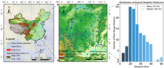
Figure 1.
The bend region of the Yellow River Basin in China and distribution of Rain Gauge Stations.
2.1. Precipitation Data
We utilize precipitation data from 123 rain gauge stations located in the bend region of the Yellow River Basin in China. These stations provide daily precipitation observations, which serve as ground truth labels for model training and validation. The observational data are obtained from the Institute of Geographic Sciences and Natural Resources Research, Chinese Academy of Sciences (https://igsnrr.cas.cn/kjpt/ptzc/sjpt (accessed on 1 November 2024)).
The ERA5-Land reanalysis precipitation dataset (0.1° × 0.1°, hourly resolution; https://cds.climate.copernicus.eu/datasets/reanalysis-era5-land?tab=download (accessed on 3 November 2024)) and the GPM_3IMERGHH_07 satellite precipitation product (0.1° × 0.1°, 30-min resolution; https://disc.gsfc.nasa.gov/datasets/GPM_3IMERGHH_07/summary?keywords=GPM (accessed on 3 November 2024)) offer relatively high spatial and temporal resolution. These datasets effectively preserve spatial precipitation patterns and exhibit strong correlation and high coefficients of determination when compared with ground-based observations [37]. The CN05.1 dataset consists of gridded daily precipitation data at 0.25° × 0.25° resolution, generated using the anomaly-based interpolation method. It is derived from observations from over 2400 meteorological stations across China and is provided by the Institute of Atmospheric Physics, Chinese Academy of Sciences (https://ccrc.iap.ac.cn/contact (accessed on 10 November 2024)) [38,39].
2.2. Multi-Source Environmental Features
The MODIS remote sensing products (1 km × 1 km, daily; https://search.earthdata.nasa.gov/search (accessed on 12 November 2024)) provide a range of cloud- and water vapor-related parameters (MOD-CWV), including Water Vapor Near-Infrared (wvni), Cloud Water Path (cwp), Cloud Optical Thickness (cot), Cloud Effective Radius (cer), Cloud Phase Infrared (cpi), Cloud Top Temperature (ctt), Cloud Top Pressure (ctp), Cloud Top Height (cth), and Surface Temperature (st). These variables directly capture the spatial distribution of cloud–water vapor–surface interactions and provide detailed and realistic spatial background information for the model. ERA5-Land environmental features (0.1° × 0.1°, daily; https://cds.climate.copernicus.eu/datasets/reanalysis-era5-land?tab=download (accessed on 20 November 2024)) offer key meteorological drivers, mainly including evaporation and evapotranspiration parameters (ERA-EVP: total evaporation (eva), evaporation from bare soil (efbs), evaporation from canopy top (efttoc), evaporation from vegetation transpiration (efvt), and potential evaporation (peva)); surface radiation and energy flux parameters (ERA-RAD: surface solar radiation downwards (ssrd), surface thermal radiation downwards (strd), surface net solar radiation (snsr), surface net thermal radiation (sntr), surface latent heat flux (slhf), surface sensible heat flux (sshf), and forecast albedo (fa)); and meteorological, vegetation, and soil parameters (ERA-MET: 2 m temperature (t2), 2 m dewpoint temperature (t2d), skin temperature (ts), 10 m u-component (u10), 10 m v-component (v10), leaf area index of high vegetation (laihv), leaf area index of low vegetation (lailv), and volumetric soil water content in layer 1 (vswl1)).
In addition, the Global Land One-kilometer Base Elevation (GLOBE) dataset, developed by the U.S. National Oceanic and Atmospheric Administration (NOAA) in collaboration with international partners [40], provides global elevation data at a resolution of 1 km × 1 km (https://www.ngdc.noaa.gov/mgg/topo/globe.html (accessed on 2 November 2024)), contributing essential topographic information for precipitation downscaling.
3. Methodology
This study proposes an Artificial Intelligence-Driven Precipitation Downscaling Method Using Spatiotemporally Coupled Multi-Source Data (AIMPD). The overall methodological framework is illustrated in Figure 2 and consists of three core modules: data processing, feature selection, and model construction and application.
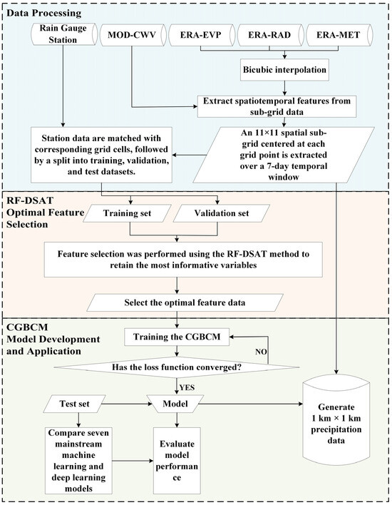
Figure 2.
Flowchart of the AI-Driven Precipitation Downscaling Method Using Spatiotemporally Coupled Multi-Source Data.
The experiments were conducted on a workstation running the Windows 11 operating system, equipped with four NVIDIA GeForce RTX 4090 GPUs and an Intel(R) Xeon(R) W9-3495X CPU. Deep learning models were implemented using the PyTorch 2.5.0 framework with CUDA 12.6 for GPU acceleration. Traditional machine learning models, including Random Forest (RF), XGBoost, and LightGBM, were implemented using the RandomForestRegressor module from scikit-learn, the XGBRegressor module from xgboost, and the LGBMRegressor module from lightgbm, respectively. To ensure reproducibility, the global random seed was fixed at 34 across all experiments.
3.1. Data Processing
First, inverse distance weighted (IDW) averaging is applied to address missing and anomalous values in the multi-source environmental feature data [41]. For missing or erroneous values in rain gauge station observations, corresponding spatiotemporal precipitation values from the CN05.1 dataset are used for imputation, with nearest-neighbor interpolation applied to match the station locations.
Second, since ERA5-Land reanalysis data, GPM_3IMERGHH_07 satellite precipitation data, and other environmental variables are recorded in Coordinated Universal Time (UTC), while ground-based observations are recorded in Beijing Time (UTC+8), all hourly products are downloaded and uniformly converted to Beijing Time to ensure temporal consistency across datasets.
Third, for each environmental variable, the minimum and maximum values over the study period are extracted, and min–max normalization is applied based on the individual value range of each variable. This linear affine transformation maps each variable to a common scale without altering the original distribution shape, thereby enhancing numerical stability and accelerating model convergence [42].
Fourth, the process of preparing model input data is illustrated in Figure 3. ERA5-Land reanalysis precipitation data, GPM_3IMERGHH_07 satellite precipitation data, and other environmental features (evaporation from canopy top (efttoc), surface net solar radiation (snsr), surface net thermal radiation (sntr), surface solar radiation downwards (ssrd), surface temperature (st), 10 m u component (u10), evaporation from bare soil (efbs), surface thermal radiation downwards (strd), 10 m v component (v10), volumetric soil water layer 1 (vswl1), and 2 m dewpoint temperature (t2d)) were resampled to a resolution of 1 km × 1 km using bicubic interpolation, producing multi-feature gridded data at a unified spatial resolution [43]. At each rain gauge station location, a local window of fixed size (e.g., 11 × 11 pixels) is extracted, and the pixel values across all variables are concatenated along the feature dimension to form a feature tensor of size number of features × 11 × 11. Feature vectors from all stations and all time steps are then sequentially arranged to construct an input matrix with shape n × (number of features × 11 × 11), which, together with the corresponding precipitation observations, constitutes the complete dataset used for model training. The dataset was subsequently divided into training, validation, and testing subsets in a ratio of 6:1:3 to ensure reliable model evaluation and generalization performance.
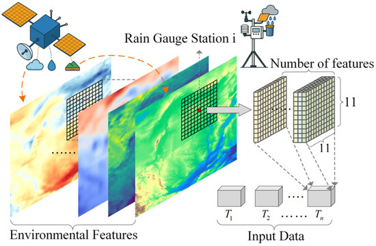
Figure 3.
Schematic diagram of data preprocessing. T1–Tn represent time series data.
3.2. Random Forest-Based Dual-Spectrum Adaptive Threshold Feature Selection Algorithm
The Random Forest-based Dual-Spectrum Adaptive Threshold feature selection algorithm (RF-DSAT) utilizes Random Forest [44] to compute feature importance and constructs two key spectra: the gradient spectrum for identifying significant breakpoints in importance, and the cumulative contribution spectrum for detecting inflection points. By integrating these two types of threshold candidate points and optimizing a scoring function that balances explained variance and complexity, the optimal feature subset threshold is determined, achieving data-driven feature selection.
3.2.1. Process Steps
- (1)
- Feature importance scores are obtained through the Random Forest model, where I represents the feature importance vector arranged in descending order of importance, and is the total number of features. Random Forest calculates the importance score of each feature by averaging impurity reduction across multiple decision trees, effectively capturing nonlinear feature relationships [45].
- (2)
- The first-order derivative of feature importance is calculated to construct the gradient spectrum, as shown in Equation (1), where represents the importance difference between adjacent features. To ensure comparability across different scales, the gradient is normalized as shown in Equation (2). Subsequently, a local extremum detection algorithm is used to identify significant change points in the gradient spectrum, as shown in Equation (3). These change points represent significant breakpoints in feature importance, indicating potential feature selection threshold positions.
- (3)
- The cumulative importance contribution of features is calculated, where represents the cumulative contribution ratio of the first features. The elbow method [46] is applied to detect the inflection point of the cumulative contribution curve (The KneeLocator function is derived from the kneed library). The inflection point position indicates where the cumulative contribution growth rate significantly decreases, representing the equilibrium point of diminishing returns.
The threshold candidate points from both the gradient spectrum and cumulative contribution spectrum are integrated, and each candidate threshold point is evaluated by optimizing the scoring function, as shown in Equation (4).
- (4)
- where represents the explained variance ratio (model performance), and represents the feature proportion penalty term (model complexity). The squared penalty term strengthens control over redundant features and tends to select more compact feature subsets.
The optimal threshold position is determined, as shown in Equation (5).
3.2.2. Experimental Design
To evaluate the effectiveness of the proposed RF-DSAT algorithm, four classical feature selection methods are employed for comparison: the Pearson correlation coefficient [47], mutual information [48], Lasso regression [49], and SHAP values [50]. The feature subsets generated by each method are used as inputs to the Artificial Intelligence-Driven Precipitation Downscaling Method Using Spatiotemporally Coupled Multi-Source Data (AIMPD). In addition, ablation experiments are conducted on different numbers of selected features to further validate the performance and robustness of RF-DSAT.
3.3. Spatiotemporally Coupled Bias Correction Model (CGBCM)
The Spatiotemporally Coupled Bias Correction Model integrates four key components: (a) a Convolutional Neural Network (CNN) module for extracting spatial features from the input data [51]; (b) a Gated Recurrent Unit (GRU) module for capturing temporal dependencies across time steps [52]; (c) a spatiotemporal coupling module that effectively integrates spatial and temporal representations; and (d) a model performance evaluation module for assessing predictive accuracy and generalization ability. The overall architecture of the proposed model is illustrated in Figure 4.
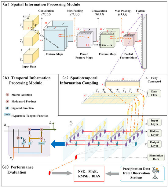
Figure 4.
Architecture diagram of the Spatiotemporally Coupled Bias Correction Model. (a) Convolutional Neural Network module, where C represents the number of features, H and W represent spatial dimensions, T represents time series, and (·,·,·) indicates the first digit represents the number of convolution kernels, the second digit represents the convolution kernel size, and the third digit represents the stride. (b) Gated Recurrent Unit structure, where h represents hidden layer data and X represents input data. (c) Spatial and temporal information coupling module. (d) Performance evaluation module.
3.3.1. Spatial Information Processing Module
Convolutional Neural Networks extract local spatial information and generate feature maps by sliding learnable convolution kernels across input feature maps. Specifically, each convolutional layer first performs convolution operations on the input tensor, then applies batch normalization and ReLU activation to enhance the model’s nonlinear representation capability [53], followed by max pooling to reduce spatial resolution while preserving the most salient features. In this model, the input multi-channel features undergo two “convolution-normalization-activation-pooling” operations, expanding the number of channels sequentially from to 15 and 30 while reducing the spatial dimensions to one-quarter of the original size. Subsequently, the resulting feature maps are flattened into vectors and mapped to hidden dimension (set to 62 in this study) through a fully connected layer.
3.3.2. Temporal Information Processing Module
Gated Recurrent Unit (GRU) is a recurrent neural network variant that efficiently captures sequential dependencies [52]. For the input vector at time step and the previous hidden state, GRU first computes the opening and closing ratios of the reset gate and update gate to control information forgetting and updating, then combines previous state information with current input to generate the candidate hidden state, and finally obtains the current hidden state through weighted fusion, as shown in Equations (6)–(9). Here, and represent the update gate and reset gate, respectively; is the candidate hidden state; is the new hidden state; , , and are the corresponding trainable weight matrices. denotes element-wise sigmoid activation function, denotes element-wise hyperbolic tangent activation function; represents vector concatenation; represents element-wise (Hadamard) multiplication; 1 is an all-ones vector with the same dimension as . The GRU structure used in this study sequentializes the D-dimensional embeddings extracted by CNN for each frame, performs recursive updates in chronological order, and treats the hidden state of the last time step as the global context vector of the entire sequence, providing temporal aggregation information for subsequent regression tasks.
3.3.3. Spatiotemporal Information Coupling Module
To fully exploit the spatiotemporal features, this study couples the CNN and GRU modules to construct an end-to-end regression model. The input samples are defined with a batch size B, temporal length T, feature channel number C, and spatial dimensions H × W. First, the original input tensor (B, T, C, H, W) is reshaped into (B × T, C, H, W), and each frame is processed through a CNN with shared parameters to extract spatial features, resulting in an intermediate representation of shape (B × T, D), where D denotes the spatial feature dimension output by the CNN. The data are then reshaped to (B, T, D) and fed into the GRU module to capture temporal dependencies along the time dimension. Finally, the final hidden state of the GRU is passed through a fully connected layer to produce a scalar prediction, with a ReLU activation applied to ensure non-negative outputs. During model training, the mean squared error (MSE) is used as the loss function, while the Adam optimizer, ReduceLROnPlateau learning rate scheduler [54,55], and gradient clipping strategies are adopted to ensure training stability and convergence.
3.3.4. CGBCM Performance Evaluation Module
To comprehensively evaluate model performance, we select the Nash-Sutcliffe efficiency coefficient (NSE), Equation (10), mean absolute error (MAE), Equation (11), root mean square error (RMSE), Equation (12), and bias (BIAS), Equation (13), as evaluation metrics. N represents the total number of samples, and and represent the -th observed value and model prediction, respectively. NSE is used to measure the consistency between simulation results and observed data, with a value range of ; the closer to 1, the better the fitting performance. MAE reflects the average absolute level of prediction errors. RMSE is more sensitive to large deviations and can highlight the impact of anomalous errors on overall performance. BIAS is used to evaluate the model’s systematic overestimation or underestimation tendency, with positive values indicating average overestimation and negative values indicating average underestimation. Model parameters and Equation (14) are used to balance the relationship between prediction accuracy and computational resource consumption for different model structures, where represents the set of all trainable parameters in the model, subscript divides these parameters by layers, and represents the dimension of parameters in the l-th layer.
3.3.5. Experimental Design
To determine the optimal structure of the CGBCM, this study first conducted a coarse-grained grid search on model depth and hyperparameters through preliminary experiments. The results indicated that optimal performance was achieved when the number of convolutional layers was set to two, the GRU depth was set to one layer, and both the number of convolution kernels and the GRU hidden dimensions were within the range of tens. Based on these observations, two-stage coordinate descent optimization experiments [56,57] were conducted using data from 2014 to analyze model structure and parameter configurations. In the first stage, the total number of convolution kernels was fixed at 45 (i.e., 15 + 30), and the GRU hidden dimension was fixed at 62. Under these conditions, the effects of different combinations of convolutional and GRU layer numbers on model performance were systematically compared. In the second stage, with the architecture fixed at (2, 1), various combinations of convolution kernel numbers and GRU hidden dimensions were further evaluated. To identify the optimal spatiotemporal configuration, the impact of different spatial window sizes (5 × 5, 11 × 11, and 17 × 17) and temporal sequence lengths (4, 7, and 10) on model performance was also systematically assessed.
After finalizing the model architecture and parameter settings, the overall performance of the Artificial Intelligence-Driven Precipitation Downscaling Method Using Spatiotemporally Coupled Multi-Source Data (AIMPD) was evaluated across the full study period (2014–2022) and compared against two categories of baseline methods. The first category includes statistical downscaling methods, specifically bicubic interpolation of ERA5-Land and GPM precipitation products (referred to as ERAPRE and IMERG, respectively). Bicubic interpolation offers superior smoothness and detail preservation compared to other classical statistical methods such as nearest-neighbor and bilinear interpolation [58]. The second category comprises hybrid approaches that combine statistical downscaling with machine learning or deep learning models. These methods share the same data processing and feature selection steps as AIMPD but differ in the bias correction model employed in the final step. For machine learning-based correction, models such as Random Forest (RF), eXtreme Gradient Boosting (XGBoost) [59], and Light Gradient Boosting Machine (LightGBM) [60] are used. For deep learning-based correction, models include Convolutional Neural Networks (CNNs), Long Short-Term Memory (LSTM) networks [61,62], Gated Recurrent Units (GRUs), and hybrid CNN–LSTM models [63]. These combined methods are named according to the model type used in the third step.
4. Results
4.1. Data Processing
Following systematic imputation and resampling, the complete dataset satisfies the “zero gaps + uniform resolution” criteria required for model training. Specifically, 0.61% of missing time steps in the original rain gauge station observation series were filled using corresponding spatiotemporal precipitation values from the CN05.1 dataset. Atmospheric water vapor (wvni), with a missing rate of 0.81%, and surface temperature (st), with 0.01% missing, were also fully recovered. For cloud microphysical variables—including cer, cot, cpi, cth, ctp, cwp, and ctt—the average missing rate was reduced from 54.6% to 0. Figure 5 compares the spatial patterns of multi-source environmental features before and after downscaling and imputation on a day with extensive missing data (22 July 2014). Using ERA5-Land shortwave radiation (ssrd) as an example, the original resolution was 0.1° (Figure 5a). After bicubic interpolation downscaling to 1 km × 1 km (Figure 5d), the spatial structure became significantly more refined. For atmospheric water vapor (wvni), the original data exhibited large areas of missing values (Figure 5b), which were effectively filled using inverse distance weighting (IDW) interpolation (Figure 5e). In the original cloud water path (cwp) data, the missing regions mainly corresponded to clear-sky pixels where satellites failed to return valid cloud microphysical observations (Figure 5c). During imputation, IDW interpolation was applied to technically missing areas (e.g., edge occlusions), while physically valid clear-sky regions were preserved as zero based on a predefined threshold (ε = 0.02 kg/m2). This strategy achieves a balance between data completeness and physical realism (Figure 5f).
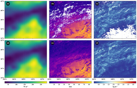
Figure 5.
Schematic diagram of spatial downscaling and missing value imputation for multi-source environmental feature data. (a) Original ERA5-Land shortwave radiation data (0.1° resolution); (d) Downscaled to 1 km × 1 km resolution after bicubic interpolation; (b) Original atmospheric water vapor data with obvious spatial missing areas; (e) Atmospheric water vapor data after imputation using inverse distance weighting method, with missing areas filled; (c) Original cloud water path data, with blank areas indicating where satellite failed to return valid values in cloud-free regions; (f) Cloud water path data after imputation, with interpolation applied to edge missing areas while preserving physical clear-sky areas as 0, achieving complete data processing.
4.2. Feature Selection Algorithm Comparison
The results of the Random Forest-Based Dual-Spectrum Adaptive Threshold (RF-DSAT) feature selection algorithm are presented in Figure 6. Using the first-order derivative method, change rate breakpoints in feature importance were detected at ranks 4, 6, 8, 11, and 14. Meanwhile, the elbow method identified an inflection point at rank 9. By integrating both approaches, the optimal number of features was determined to be 11. This comprehensive feature selection strategy effectively balances model dimensionality and explanatory power. The selected 11 features account for 78.45% of the total variance in the target variable, capturing the majority of the information structure in the original dataset while substantially reducing feature dimensionality.
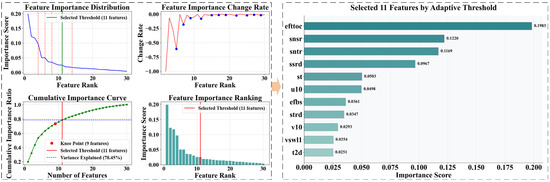
Figure 6.
Ranking results of the Random Forest-based Dual-Spectrum Adaptive Threshold feature selection algorithm. efttoc: evaporation from canopy top, snsr: surface net solar radiation, sntr: surface net thermal radiation, ssrd: surface solar radiation downwards, st: Surface Temperature, u10: 10m u component, efbs: evaporation from bare soil, strd: surface thermal radiation downwards, v10: 10m v component, vswl1: Volumetric soil water layer 1, t2d: 2m dewpoint temperature.
The feature ranking results produced by the five selection algorithms are illustrated in Figure 7, where black boxes indicate the top 11 features identified by each method. Figure 8 presents a comparative evaluation of the feature selection algorithms. Among them, the 11 features selected by the Random Forest algorithm yielded the best model performance, achieving a Nash–Sutcliffe Efficiency (NSE) of 0.9324, a Mean Absolute Error (MAE) of 0.4752, and a Root Mean Square Error (RMSE) of 1.2052, significantly outperforming the other methods. Ablation experiments further demonstrated that altering the number of selected features—either by reducing it to 10 or increasing it to 12—resulted in a decline in model performance. This confirms that selecting 11 features offers an optimal balance between information sufficiency and redundancy control.
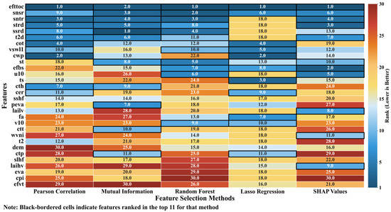
Figure 7.
Feature importance ranking under different feature selection algorithms. wvni: Water Vapor Near-Infrared, cwp: Cloud Water Path, cot: Cloud Optical Thickness, cer: Cloud Effective Radius, cpi: Cloud Phase Infrared, ctt: Cloud Top Temperature, ctp: Cloud Top Pressure, cth: Cloud Top Height, st: Surface Temperature, eva: total evaporation, efbs: evaporation from bare soil, efttoc: evaporation from canopy top, efvt: evaporation from vegetation transpiration, peva: potential evaporation, ssrd: surface solar radiation downwards, strd: surface thermal radiation downwards, snsr: surface net solar radiation, sntr: surface net thermal radiation, slhf: surface latent heat flux, sshf: surface sensible heat flux, fa: Forecast albedo, t2: 2m temperature, t2d: 2m dewpoint temperature, ts: skin temperature, u10: 10m u component, v10: 10m v component, laihv: Leaf area index high vegetation, lailv: Leaf area index low vegetation, vswl1: Volumetric soil water layer 1.
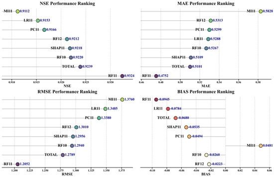
Figure 8.
Model performance metric ranking under different feature selection strategies. RF: Random Forest, SHAP: SHapley Additive exPlanations, PC: Pearson Correlation coefficient, MI: Mutual Information, LR: Lasso Regression, TOTAL: All features, RF11: The number following represents the number of selected features.
In terms of algorithm comparison, Random Forest achieved the highest NSE (0.9324), followed by SHAP (0.9218), the Pearson correlation coefficient (0.9166), and Lasso regression (0.9153). Mutual information showed the weakest performance, with an NSE of 0.9112. Notably, the model trained using all available features (NSE = 0.9239) performed worse than the one trained using the 11 features selected by Random Forest, underscoring the necessity and effectiveness of the feature selection process. Although Random Forest exhibited slightly higher bias in certain cases, its overall predictive performance was superior.
4.3. CGBCM Model Configuration and Spatiotemporal Perception Scale
4.3.1. Model Structure and Hyperparameter Configuration
The results of the first-stage experiments are presented in Figure 9. The structure (2,1)—where the first digit denotes the number of convolutional layers and the second the number of GRU hidden layers (notation consistent throughout this section)—significantly outperformed other configurations. It achieved an NSE of 0.9324, with MAE and RMSE reduced to 0.4752 and 1.2052, respectively, and a BIAS of −0.0945. In comparison, the (1,1) structure was too shallow, resulting in a decreased NSE of 0.9200 and an increased RMSE of 1.3109. Increasing the number of convolutional layers to three also failed to improve performance; both (3,1) and (3,2) yielded NSE values below 0.912. These results suggest that the moderate-depth configuration (2,1) offers the best trade-off between performance and complexity, with only 36,941 parameters, making it highly practical for implementation.
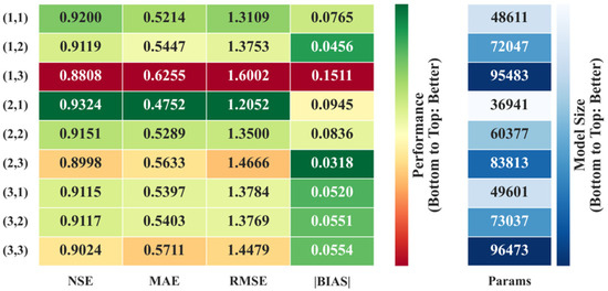
Figure 9.
CGBCM performance comparison under different combinations of convolutional and GRU layer numbers. (·,·) The first digit represents the number of convolutional layers, the second digit represents the number of hidden layers.
The second-stage experimental results, shown in Figure 10, indicate that the (15,30,62) parameter combination—where the first and second digits represent the number of kernels in the first and second convolutional layers, respectively, and the third digit denotes the GRU hidden dimension—achieved the best overall performance. In contrast, the smaller configuration (10,20,31) resulted in a significantly lower NSE of 0.9075 due to insufficient model capacity. The larger setting (20,40,93), despite increased capacity, did not lead to performance improvement and showed a reduced NSE of 0.9193. The (15,30,62) configuration achieved performance nearly equivalent to the largest tested setup (15,30,93), which had an NSE of 0.9355, while requiring nearly half the number of parameters (approximately 36,941 vs. 69,739), thus offering substantial reductions in computational cost with negligible accuracy loss (Figure 11).
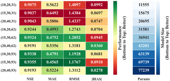
Figure 10.
CGBCM performance comparison under different combinations of convolution kernels and GRU hidden dimensions. (·,·,·) The first digit represents the number of kernels in the first convolutional layer, the second digit represents the number of kernels in the second convolutional layer, the third digit represents the hidden layer dimension.
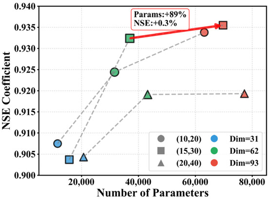
Figure 11.
Balance performance between accuracy and computational cost under different structural combinations. (·,·) The first digit represents the number of kernels in the first convolutional layer, the second digit represents the number of kernels in the second convolutional layer. The red arrow indicates the improvement of NSE after model optimization.
In summary, the structure (2,1) and parameter combination (15,30,62), obtained through a two-stage coordinate descent process, significantly reduced error and systematic bias while maintaining high simulation accuracy and controlling model complexity.
4.3.2. Spatial Perception Scale and Temporal Modeling Span
Regarding spatial perception, the intermediate receptive field size of 11 × 11 achieved the best overall performance, yielding an NSE of 0.9324, an MAE of 0.4752, an RMSE of 1.2052, and a BIAS of −0.0945 under a temporal sequence length of 7 (Figure 12). In contrast, the smaller 5 × 5 window, although computationally efficient, exhibited limited spatial coverage and slightly reduced performance. Meanwhile, the larger 17 × 17 window led to performance degradation due to the inclusion of excessive spatial redundancy and noise, with the NSE dropping to 0.8942. In the temporal dimension, a sequence length of 7 consistently produced superior results across all spatial configurations. Shorter sequences (length = 4) failed to capture sufficient temporal dependencies, resulting in generally lower accuracy. On the other hand, longer sequences (length = 10) introduced temporal non-stationarity, which negatively affected model performance.
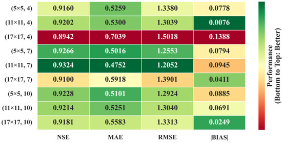
Figure 12.
Model performance evaluation results under different combinations of spatial windows and temporal sequence lengths. (·×·, ·) The first × represents spatial window size, the second represents temporal sequence length.
Overall, the combination of an 11 × 11 spatial window and a temporal sequence length of 7 demonstrated the optimal balance between modeling accuracy and error control.
5. Discussion
As shown in Figure 13, the AI-Driven Precipitation Downscaling Method Using Spatiotemporally Coupled Multi-Source Data (AIMPD) consistently outperformed the bicubic interpolation method in simulating precipitation during 2014–2022. The NSE remained stable between 0.85 and 0.93, while the mean absolute error (MAE) and root mean square error (RMSE) ranged from 0.47 to 0.56 mm and from 1.20 to 1.70 mm, respectively. BIAS was close to zero, indicating excellent agreement with ground-based observations and the absence of significant systematic deviation. Among the baseline methods, ERAPRE performed second best, with NSE values ranging from 0.55 to 0.73, MAE between approximately 0.87 and 1.00 mm, RMSE between 2.3 and 3.6 mm, and an annual average BIAS of 0.09 mm. In contrast, IMERG exhibited the weakest performance, with NSE between 0.50 and 0.69, MAE rising to 1.92–3.68 mm, RMSE increasing to 5.57–12.12 mm, and persistent BIAS in the range of 1.33–3.20 mm. In terms of interannual variation, AIMPD demonstrated the highest stability, with minimal fluctuations across all evaluation metrics. Scatter plot analysis further revealed that although all three datasets showed increased absolute error under high precipitation intensities, IMERG was particularly sensitive, whereas AIMPD maintained relatively low error even in extreme precipitation conditions. The bicubic interpolation method, while computationally simple, only performs geometric smoothing. It neither corrects systematic errors in satellite data nor incorporates atmospheric dynamics, radiation, or related physical mechanisms. As a result, it tends to produce spatial artifacts under heavy precipitation and generates false rain signals in weak or dry conditions. In summary, AIMPD offers substantial advantages over bicubic interpolation in terms of accuracy, robustness, and systematic error control, making it a more reliable approach for high-resolution precipitation downscaling across varying hydrometeorological conditions.
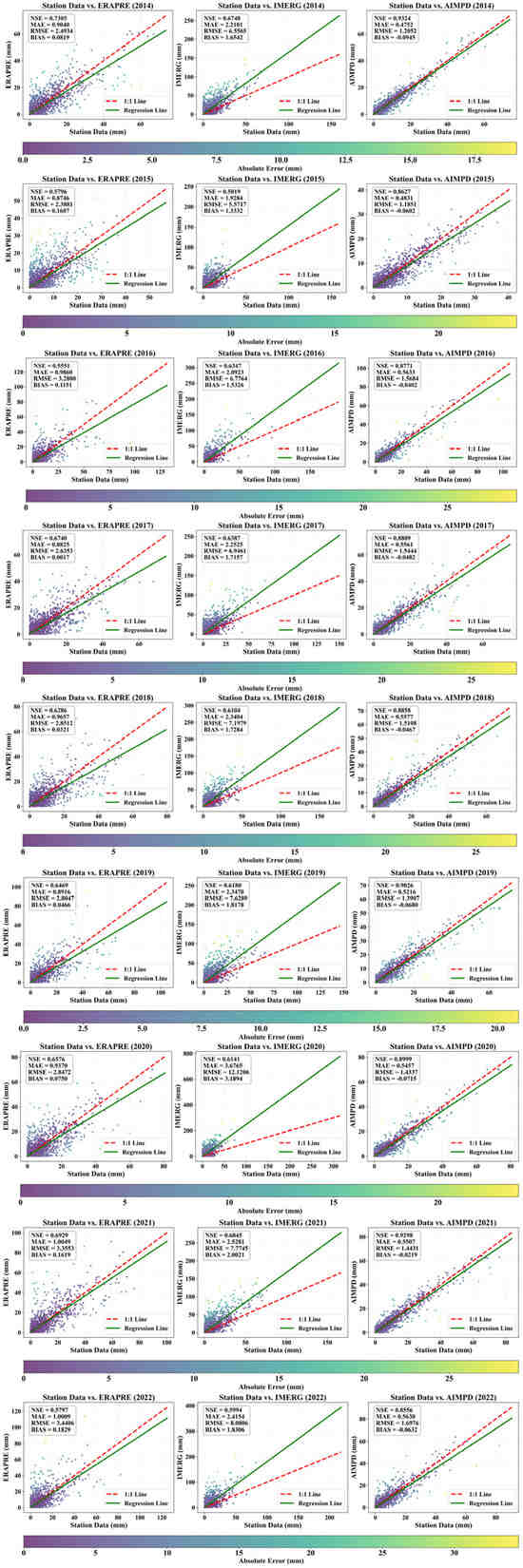
Figure 13.
Comparison scatter plots and statistical metrics of Rain Gauge Station observation data versus ERAPRE, IMERG, and AIMPD simulated precipitation data during 2014–2022.
Figure 14 shows the mean daily precipitation averaged over 123 rain gauge stations in the study area in 2014. Based on these data, four representative days were selected for spatial comparison: heavy precipitation on 11 September, moderate on 29 June, light on 28 March, and no precipitation on 17 January. Figure 15 displays the corresponding spatial precipitation fields simulated by ERAPRE, IMERG, and AIMPD. The results indicate that AIMPD consistently produced precipitation fields that closely matched observations across all precipitation intensities. Under heavy precipitation conditions (26.1 mm), AIMPD accurately captured the core rainfall zones while effectively avoiding spurious artifacts. For moderate and light precipitation events, it reliably reproduced the primary precipitation belts, whereas ERAPRE and IMERG tended to either overestimate the spatial extent or miss localized rainfall patterns. Notably, on no-precipitation days, AIMPD maintained near-zero values across the domain, while both benchmark products exhibited residual rain spot artifacts. These findings demonstrate that AIMPD achieves superior spatial accuracy and noise suppression under varying rainfall regimes, significantly outperforming bicubic interpolation and conventional satellite-based products.
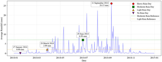
Figure 14.
Average daily precipitation of 123 rain gauge stations within the study area in 2014.
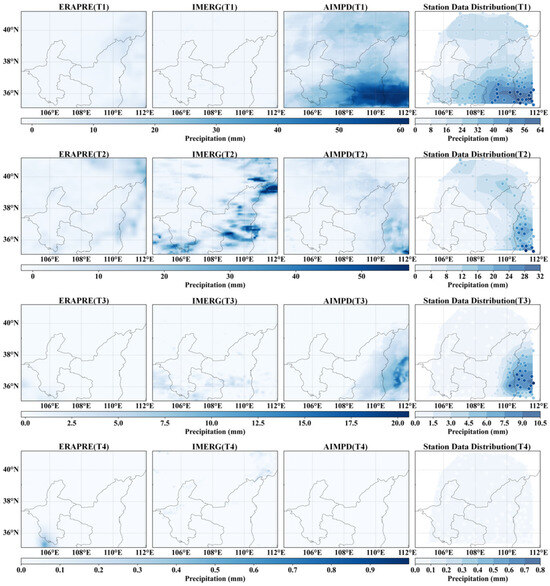
Figure 15.
Spatial distribution comparison of ERAPRE, IMERG, and AIMPD simulated data with Rain Gauge Station observation data under four precipitation intensity scenarios (heavy, moderate, light, and no precipitation) in 2014. Four representative dates are marked in the figure: T1; (11 September 2014), T2 (29 June 2014), T3 (28 March 2014), and T4 (17 January 2014).
AIMPD was compared with several methods combining statistical downscaling and machine learning or deep learning models, including Random Forest (RF), eXtreme Gradient Boosting (XGBoost), Light Gradient Boosting Machine (LightGBM), Convolutional Neural Networks (CNNs), Long Short-Term Memory (LSTM) networks, Gated Recurrent Units (GRUs), and hybrid CNN–LSTM models. As shown in Figure 16 and Figure 17, AIMPD exhibited overall superior performance. In this study, both model training and validation were conducted using daily precipitation data, and all performance metrics (NSE, MAE, RMSE, and BIAS) were calculated at the daily scale. In Equations (10)–(13), N represents the number of days in a year. The calculated indicators therefore reflect the overall model performance for each year based on daily-scale evaluations. Presenting the results on an annual basis provides a clearer view of the model’s overall performance across different years. Its average annual NSE reached 0.8919, which is 1.73% higher than that of the second-ranked CNN–LSTM (0.8767) and 8.73% higher than CNN (0.8203), the lowest-performing model. In terms of error metrics, AIMPD achieved an MAE of 0.5352 mm and an RMSE of 1.4421 mm, representing reductions of 9.96% and 6.48% compared to CNN–LSTM, and 19.91% and 22.19% compared to CNN. Although CNN achieved slightly lower absolute bias (|BIAS| = 0.0404 mm), its overall performance—reflected by lower NSE and higher errors (MAE = 0.6682 mm, RMSE = 1.8534 mm)—was comparatively poor. Relative to XGBoost, LightGBM, and RF, AIMPD also maintained consistent advantages across all metrics while controlling BIAS within 0.0572 mm, further validating its robustness and accuracy.
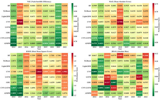
Figure 16.
Comparison of precipitation simulation performance metrics for various methods during 2014–2022.
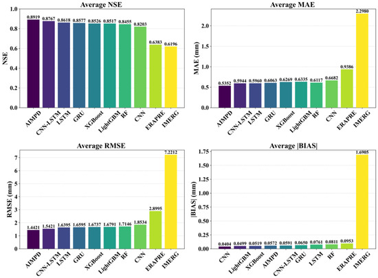
Figure 17.
Comparison of average performance metrics for various methods during 2014–2022.
This result is consistent with previous studies. Wu et al. (2020) [64] and Gavahi et al. (2023) [33] pointed out that the CNN–LSTM architecture can capture the spatial and temporal dependencies of precipitation more effectively than single CNN or LSTM models. However, compared with GRU, the LSTM network is more complex and parameter-intensive, making it more prone to overfitting [33,64]. Zhang et al. (2024) [27] also found in their machine learning-based multi-source downscaling study that, although tree-based models have certain advantages in multi-source data fusion, they lack temporal mechanisms and thus fail to represent the dynamic evolution of precipitation processes [27]. In contrast, the AIMPD model integrates the advantages of multi-source physical features and spatiotemporal dependency structures. Eleven cloud–radiation–dynamics features selected through RF-DSAT are directly input into the model, two CNN layers capture local gradients within an 11 × 11 receptive field, and a single GRU layer extracts temporal dependencies within a seven-day window, effectively suppressing the propagation and amplification of random errors in space and time. This structural design is also supported by other studies, as Gavahi et al. (2023) [33] and Zhang et al. (2024) [27] demonstrated that combining CNN and recurrent neural structures can significantly improve the accuracy and stability of downscaling models.
The primary limitation of the proposed method lies in its current implementation for a single spatial resolution of 1 km × 1 km, with auxiliary variables also constrained to MODIS products at the same resolution. Although this ensures consistency and accuracy of spatial information at this scale, it restricts the model’s flexibility to accommodate varying application demands—ranging from fine-scale urban analyses to broader regional assessments. Future research could explore the integration of multi-source data across diverse spatial resolutions. For instance, MODIS 500 m × 500 m surface reflectance, Sentinel imagery, and higher-resolution products such as Landsat (e.g., 250 m × 250 m) could be incorporated to support enhanced downscaling targets. By reconstructing a hierarchical multi-resolution feature framework, the model can be extended to support flexible and adaptive precipitation downscaling at various spatial scales, thereby improving its applicability in multi-scale hydrometeorological applications.
6. Conclusions
This study innovatively proposes an AI-Driven Precipitation Downscaling Method Using Spatiotemporally Coupled Multi-Source Data (AIMPD). Based on unifying spatiotemporal resolution, completing missing values, and extracting local spatial information, the method utilizes the RF-DSAT algorithm to precisely select optimal auxiliary features and constructs a spatiotemporally coupled bias correction model for multi-source data, achieving high-precision downscaling of precipitation data from 0.1° × 0.1° to 1 km × 1 km resolution. Compared to statistical downscaling methods and their machine learning or deep learning variants, it consistently outperforms across all evaluation metrics, particularly in accurately restoring spatial distributions during extreme precipitation events. The method achieves higher accuracy with minimal parameters, providing strong support for fine-scale meteorological data applications.
Author Contributions
Conceptualization, C.L., L.M., X.H. and Q.Z.; methodology, C.L. and L.M.; software, C.L.; validation, C.L.; formal analysis, C.L.; investigation, C.L., L.M., X.H., C.W., X.L. and B.S.; resources, L.M.; data curation, C.L., C.W., X.L. and B.S.; visualization, C.L., C.W., X.L. and B.S.; writing—original draft preparation, C.L.; writing—review and editing, L.M. and X.H.; supervision, L.M., X.H. and Q.Z.; project administration, L.M. and X.H.; funding acquisition, L.M. All authors have read and agreed to the published version of the manuscript.
Funding
This work was supported by the National Key R&D Program of China (Grant No. 2023YFC3206502), and by the First-class Academic Subjects Special Research Project of the Education Department of Inner Mongolia Autonomous Region (Grant No. YLXKZX-NND-010).
Institutional Review Board Statement
Not applicable.
Informed Consent Statement
Not applicable.
Data Availability Statement
The raw data supporting the conclusions of this article will be made available by the authors on request.
Conflicts of Interest
The authors declare no conflicts of interest.
References
- Vogel, R.M.; Lall, U.; Cai, X.M.; Rajagopalan, B.; Weiskel, P.K.; Hooper, R.P.; Matalas, N.C. Hydrology: The interdisciplinary science of water. Water Resour. Res. 2015, 51, 4409–4430. [Google Scholar] [CrossRef]
- Feldman, A.F.; Feng, X.; Felton, A.J.; Konings, A.G.; Knapp, A.K.; Biederman, J.A.; Poulter, B. Plant responses to changing rainfall frequency and intensity. Nat. Rev. Earth Environ. 2024, 5, 276–294. [Google Scholar] [CrossRef]
- Strohmenger, L.; Ackerer, P.; Belfort, B.; Pierret, M.C. Local and seasonal climate change and its influence on the hydrological cycle in a mountainous forested catchment. J. Hydrol. 2022, 610, 127914. [Google Scholar] [CrossRef]
- Antal, A.; Guerreiro, P.M.P.; Cheval, S. Comparison of spatial interpolation methods for estimating the precipitation distribution in Portugal. Theor. Appl. Climatol. 2021, 145, 1193–1206. [Google Scholar] [CrossRef]
- Xiang, Y.X.; Zeng, C.; Zhang, F.; Wang, L. Effects of climate change on runoff in a representative Himalayan basin assessed through optimal integration of multi-source precipitation data. J. Hydrol.-Reg. Stud. 2024, 53, 101828. [Google Scholar] [CrossRef]
- Jongjin, B.; Jongmin, P.; Dongryeol, R.; Minha, C. Geospatial blending to improve spatial mapping of precipitation with high spatial resolution by merging satellite-based and ground-based data. Hydrol. Process 2016, 30, 2789–2803. [Google Scholar] [CrossRef]
- Lei, H.J.; Zhao, H.Y.; Ao, T.Q. Ground validation and error decomposition for six state-of-the-art satellite precipitation products over mainland China. Atmos. Res. 2022, 269, 106017. [Google Scholar] [CrossRef]
- Moazami, S.; Na, W.Y.; Najafi, M.R.; de Souza, C. Spatiotemporal bias adjustment of IMERG satellite precipitation data across Canada. Adv. Water Resour. 2022, 168, 104300. [Google Scholar] [CrossRef]
- Gebremichael, M.; Bitew, M.M.; Hirpa, F.A.; Tesfay, G.N. Accuracy of satellite rainfall estimates in the Blue Nile Basin: Lowland plain versus highland mountain. Water Resour. Res. 2014, 50, 8775–8790. [Google Scholar] [CrossRef]
- Li, M.; Shao, Q.X. An improved statistical approach to merge satellite rainfall estimates and raingauge data. J. Hydrol. 2010, 385, 51–64. [Google Scholar] [CrossRef]
- Prein, A.F.; Gobiet, A. Impacts of uncertainties in European gridded precipitation observations on regional climate analysis. Int. J. Climatol. 2017, 37, 305–327. [Google Scholar] [CrossRef] [PubMed]
- Bao, J.W.; Feng, J.M.; Wang, Y.L. Dynamical downscaling simulation and future projection of precipitation over China. J. Geophys. Res.-Atmos. 2015, 120, 8227–8243. [Google Scholar] [CrossRef]
- Politi, N.; Vlachogiannis, D.; Sfetsos, A.; Nastos, P.T. High-resolution dynamical downscaling of ERA-Interim temperature and precipitation using WRF model for Greece. Clim. Dynam 2021, 57, 799–825. [Google Scholar] [CrossRef]
- Gao, S.B.; Huang, D.L.; Du, N.Z.; Ren, C.Y.; Yu, H.Q. WRF ensemble dynamical downscaling of precipitation over China using different cumulus convective schemes. Atmos. Res. 2022, 271, 106116. [Google Scholar] [CrossRef]
- Xue, Y.K.; Janjic, Z.; Dudhia, J.; Vasic, R.; De Sales, F. A review on regional dynamical downscaling in intraseasonal to seasonal simulation/prediction and major factors that affect downscaling ability. Atmos. Res. 2014, 147, 68–85. [Google Scholar] [CrossRef]
- Adachi, S.A.; Tomita, H. Methodology of the Constraint Condition in Dynamical Downscaling for Regional Climate Evaluation: A Review. J. Geophys. Res.-Atmos. 2020, 125, e2019JD032166. [Google Scholar] [CrossRef]
- Maraun, D.; Wetterhall, F.; Ireson, A.M.; Chandler, R.E.; Kendon, E.J.; Widmann, M.; Brienen, S.; Rust, H.W.; Sauter, T.; Themessl, M.; et al. Precipitation Downscaling under Climate Change: Recent Developments to Bridge the Gap between Dynamical Models and the End User. Rev. Geophys. 2010, 48, Rg3003. [Google Scholar] [CrossRef]
- Rastogi, D.; Niu, H.R.; Passarella, L.; Mahajan, S.; Kao, S.C.; Vahmani, P.; Jones, A.D. Complementing Dynamical Downscaling With Super-Resolution Convolutional Neural Networks. Geophys. Res. Lett. 2025, 52, e2024GL111828. [Google Scholar] [CrossRef]
- Vosper, E.; Watson, P.; Harris, L.; McRae, A.; Santos-Rodriguez, R.; Aitchison, L.; Mitchell, D. Deep Learning for Downscaling Tropical Cyclone Rainfall to Hazard-Relevant Spatial Scales. J. Geophys. Res.-Atmos. 2023, 128, e2022JD038163. [Google Scholar] [CrossRef]
- Liu, X.L.; Coulibaly, P.; Evora, N. Comparison of data-driven methods for downscaling ensemble weather forecasts. Hydrol. Earth Syst. Sci. 2008, 12, 615–624. [Google Scholar] [CrossRef]
- Vrac, M.; Drobinski, P.; Merlo, A.; Herrmann, M.; Lavaysse, C.; Li, L.; Somot, S. Dynamical and statistical downscaling of the French Mediterranean climate: Uncertainty assessment. Nat. Hazard. Earth Syst. Sci. 2012, 12, 2769–2784. [Google Scholar] [CrossRef]
- Sarhadi, A.; Burn, D.H.; Yang, G.; Ghodsi, A. Advances in projection of climate change impacts using supervised nonlinear dimensionality reduction techniques. Clim. Dynam 2017, 48, 1329–1351. [Google Scholar] [CrossRef]
- Lima, C.H.R.; Kwon, H.H.; Kim, H.J. Sparse Canonical Correlation Analysis Postprocessing Algorithms for GCM Daily Rainfall Forecasts. J. Hydrometeorol. 2022, 23, 1705–1718. [Google Scholar] [CrossRef]
- Peleg, N.; Molnar, P.; Burlando, P.; Fatichi, S. Exploring stochastic climate uncertainty in space and time using a gridded hourly weather generator. J. Hydrol. 2019, 571, 627–641. [Google Scholar] [CrossRef]
- Wang, F.; Tian, D.; Lowe, L.; Kalin, L.; Lehrter, J. Deep Learning for Daily Precipitation and Temperature Downscaling. Water Resour. Res. 2021, 57, e2020WR029308. [Google Scholar] [CrossRef]
- Ghorbanpour, A.K.; Hessels, T.; Moghim, S.; Afshar, A. Comparison and assessment of spatial downscaling methods for enhancing the accuracy of satellite-based precipitation over Lake Urmia Basin. J. Hydrol. 2021, 596, 126055. [Google Scholar] [CrossRef]
- Zhang, X.; Song, Y.; Nam, W.H.; Huang, T.L.; Gu, X.H.; Zeng, J.Y.; Huang, S.Z.; Chen, N.C.; Yan, Z.; Niyogi, D. Data fusion of satellite imagery and downscaling for generating highly fine-scale precipitation. J. Hydrol. 2024, 631, 130665. [Google Scholar] [CrossRef]
- Zhu, H.L.; Liu, H.Z.; Zhou, Q.M.; Cui, A.H. Towards an Accurate and Reliable Downscaling Scheme for High-Spatial-Resolution Precipitation Data. Remote Sens. 2023, 15, 2640. [Google Scholar] [CrossRef]
- Zhu, H.L.; Zhou, Q.M. Advancing Satellite-Derived Precipitation Downscaling in Data-Sparse Area Through Deep Transfer Learning. IEEE Trans. Geosci. Remote Sens. 2024, 62, 4102513. [Google Scholar] [CrossRef]
- Baño-Medina, J.; Manzanas, R.; Gutiérrez, J.M. Configuration and intercomparison of deep learning neural models for statistical downscaling. Geosci. Model. Dev. 2020, 13, 2109–2124. [Google Scholar] [CrossRef]
- Liu, Z.Y.; Yang, Q.L.; Shao, J.M.; Wang, G.Q.; Liu, H.Y.; Tang, X.P.; Xue, Y.H.; Bai, L.L. Improving daily precipitation estimation in the data scarce area by merging rain gauge and TRMM data with a transfer learning framework. J. Hydrol. 2022, 613, 128455. [Google Scholar] [CrossRef]
- Gu, J.J.; Ye, Y.T.; Jiang, Y.Z.; Dong, J.P.; Cao, Y.; Huang, J.X.; Guan, H.Z. A downscaling-calibrating framework for generating gridded daily precipitation estimates with a high spatial resolution. J. Hydrol. 2023, 626, 130371. [Google Scholar] [CrossRef]
- Gavahi, K.; Foroumandi, E.; Moradkhani, H. A deep learning-based framework for multi-source precipitation fusion. Remote Sens. Environ. 2023, 295, 113723. [Google Scholar] [CrossRef]
- Asfaw, T.G.; Luo, J.J. Downscaling Seasonal Precipitation Forecasts over East Africa with Deep Convolutional Neural Networks. Adv. Atmos. Sci. 2024, 41, 449–464. [Google Scholar] [CrossRef]
- Jiang, Y.Z.; Yang, K.; Qi, Y.C.; Zhou, X.; He, J.; Lu, H.; Li, X.; Chen, Y.Y.; Li, X.D.; Zhou, B.R.; et al. TPHiPr: A long-term (1979-2020) high-accuracy precipitation dataset (1/30°, daily) for the Third Pole region based on high-resolution atmospheric modeling and dense observations. Earth Syst. Sci. Data 2023, 15, 621–638. [Google Scholar] [CrossRef]
- Wang, Z.X.; Mao, Y.D.; Geng, J.Z.; Huang, C.J.; Ogg, J.; Kemp, D.B.; Zhang, Z.; Pang, Z.B.; Zhang, R. Pliocene-Pleistocene evolution of the lower Yellow River in eastern North China: Constraints on the age of the Sanmen Gorge connection. Glob. Planet. Change 2022, 213, 103835. [Google Scholar] [CrossRef]
- Zhou, H.W.; Ning, S.; Li, D.; Pan, X.S.; Li, Q.; Zhao, M.; Tang, X. Assessing the Applicability of Three Precipitation Products, IMERG, GSMaP, and ERA5, in China over the Last Two Decades. Remote Sens. 2023, 15, 4154. [Google Scholar] [CrossRef]
- Wu, J.; Gao, X.J.; Giorgi, F.; Chen, D.L. Changes of effective temperature and cold/hot days in late decades over China based on a high resolution gridded observation dataset. Int. J. Climatol. 2017, 37, 788–800. [Google Scholar] [CrossRef]
- Xu, Y.; Gao, X.J.; Shen, Y.; Xu, C.H.; Shi, Y.; Giorgi, F. A Daily Temperature Dataset over China and Its Application in Validating a RCM Simulation. Adv. Atmos. Sci. 2009, 26, 763–772. [Google Scholar] [CrossRef]
- Hastings, D.A.; Dunbar, P.K.; Elphingstone, G.M.; Bootz, M.; Murakami, H.; Maruyama, H.; Masaharu, H.; Holland, P.; Payne, J.; Bryant, N.A. The Global Land One-Kilometer Base Elevation (GLOBE) Digital Elevation Model, Version 1.0; National Oceanic and Atmospheric Administration: Silver Spring, MD, USA; National Geophysical Data Center: Boulder, CO, USA, 1999; Volume 325, pp. 80305–83328. [Google Scholar]
- Jing, Y.H.; Lin, L.P.; Li, X.H.; Li, T.W.; Shen, H.F. An attention mechanism based convolutional network for satellite precipitation downscaling over China. J. Hydrol. 2022, 613, 128388. [Google Scholar] [CrossRef]
- Zhang, H.X.; Huo, S.L.; Feng, L.; Ma, C.Z.; Li, W.P.; Liu, Y.; Wu, F.C. Geographic Characteristics and Meteorological Factors Dominate the Variation of Chlorophyll-a in Lakes and Reservoirs With Higher TP Concentrations. Water Resour. Res. 2024, 60, e2023WR036587. [Google Scholar] [CrossRef]
- Zhang, M.; Wu, B.F.; Zeng, H.W.; He, G.J.; Liu, C.; Tao, S.Q.; Zhang, Q.; Nabil, M.; Tian, F.Y.; Bofana, J.; et al. GCI30: A global dataset of 30 m cropping intensity using multisource remote sensing imagery. Earth Syst. Sci. Data 2021, 13, 4799–4817. [Google Scholar] [CrossRef]
- Breiman, L. Random forests. Mach. Learn. 2001, 45, 5–32. [Google Scholar] [CrossRef]
- Yuan, X.G.; Liu, S.R.; Feng, W.; Dauphin, G. Feature Importance Ranking of Random Forest-Based End-to-End Learning Algorithm. Remote Sens. 2023, 15, 5203. [Google Scholar] [CrossRef]
- Liu, F.; Deng, Y. Determine the Number of Unknown Targets in Open World Based on Elbow Method. IEEE Trans. Fuzzy Syst. 2021, 29, 986–995. [Google Scholar] [CrossRef]
- Pearson, K. Notes on the history of correlation. Biometrika 1920, 13, 25–45. [Google Scholar] [CrossRef]
- Shannon, C.E. A mathematical theory of communication. Bell Syst. Tech. J. 1948, 27, 379–423. [Google Scholar] [CrossRef]
- Tibshirani, R. Regression shrinkage and selection via the lasso. J. R. Stat. Soc. Ser. B Stat. Methodol. 1996, 58, 267–288. [Google Scholar] [CrossRef]
- Lundberg, S.M.; Lee, S.I. A Unified Approach to Interpreting Model Predictions. In Proceedings of the 31st International Conference on Neural Information Processing Systems (NIPS’17), Long Beach, CA, USA, 4–9 December 2017; Volume 30. [Google Scholar] [CrossRef]
- LeCun, Y.; Bottou, L.; Bengio, Y.; Haffner, P. Gradient-based learning applied to document recognition. Proc. IEEE 2002, 86, 2278–2324. [Google Scholar] [CrossRef]
- Cho, K.; Van Merriënboer, B.; Gulcehre, C.; Bahdanau, D.; Bougares, F.; Schwenk, H.; Bengio, Y. Learning phrase representations using RNN encoder-decoder for statistical machine translation. arXiv 2014, arXiv:1406.1078. [Google Scholar] [CrossRef]
- Krizhevsky, A.; Sutskever, I.; Hinton, G.E. ImageNet Classification with Deep Convolutional Neural Networks. Commun. ACM 2017, 60, 84–90. [Google Scholar] [CrossRef]
- Kingma, D.P.; Ba, J. Adam: A method for stochastic optimization. arXiv 2014, arXiv:1412.6980. [Google Scholar] [CrossRef]
- Iiduka, H. Appropriate Learning Rates of Adaptive Learning Rate Optimization Algorithms for Training Deep Neural Networks. IEEE Trans. Cybern. 2022, 52, 13250–13261. [Google Scholar] [CrossRef] [PubMed]
- Wright, S.J. Coordinate descent algorithms. Math. Program. 2015, 151, 3–34. [Google Scholar] [CrossRef]
- Nesterov, Y. Efficiency of Coordinate Descent Methods on Huge-Scale Optimization Problems. SIAM J. Optimiz. 2012, 22, 341–362. [Google Scholar] [CrossRef]
- Keys, R. Cubic convolution interpolation for digital image processing. IEEE Trans. Acoust. Speech Signal Process. 2003, 29, 1153–1160. [Google Scholar] [CrossRef]
- Chen, T.Q.; Guestrin, C. XGBoost: A Scalable Tree Boosting System. In Kdd’16: Proceedings of the 22nd Acm Sigkdd International Conference on Knowledge Discovery and Data Mining, San Francisco, CA, USA, 13–17 August 2016; Association for Computing Machinery: New York, NY, USA, 2016; pp. 785–794. [Google Scholar] [CrossRef]
- Ke, G.L.; Meng, Q.; Finley, T.; Wang, T.F.; Chen, W.; Ma, W.D.; Ye, Q.W.; Liu, T.Y. LightGBM: A Highly Efficient Gradient Boosting Decision Tree. In Proceedings of the 31st International Conference on Neural Information Processing Systems (NIPS’17), Auckland, New Zealand, 4–9 December 2017; Volume 30. [Google Scholar]
- Hochreiter, S.; Schmidhuber, J. Long short-term memory. Neural Comput. 1997, 9, 1735–1780. [Google Scholar] [CrossRef]
- Gers, F.A.; Schmidhuber, J.; Cummins, F. Learning to forget: Continual prediction with LSTM. Neural Comput. 2000, 12, 2451–2471. [Google Scholar] [CrossRef]
- Shi, X.J.; Chen, Z.R.; Wang, H.; Yeung, D.Y.; Wong, W.K.; Woo, W.C. Convolutional LSTM Network: A Machine Learning Approach for Precipitation Nowcasting. In Advances in Neural Information Processing Systems 28 (Nips 2015), Proceedings of the 29th International Conference on Neural Information Processing Systems, Montreal, QC, Canada, 7 December 2015; Curran Associates, Inc.: Red Hook, NY, USA, 2015; Volume 28. [Google Scholar]
- Wu, H.C.; Yang, Q.L.; Liu, J.M.; Wang, G.Q. A spatiotemporal deep fusion model for merging satellite and gauge precipitation in China. J. Hydrol. 2020, 584, 124664. [Google Scholar] [CrossRef]


Disclaimer/Publisher’s Note: The statements, opinions and data contained in all publications are solely those of the individual author(s) and contributor(s) and not of MDPI and/or the editor(s). MDPI and/or the editor(s) disclaim responsibility for any injury to people or property resulting from any ideas, methods, instructions or products referred to in the content. |
© 2025 by the authors. Licensee MDPI, Basel, Switzerland. This article is an open access article distributed under the terms and conditions of the Creative Commons Attribution (CC BY) license (https://creativecommons.org/licenses/by/4.0/).