Application of Hybrid Data Assimilation Methods for Mesoscale Eddy Simulation and Prediction in the South China Sea

Abstract

In this study, we compare two novel hybrid data assimilation (DA) methods: Localized Weighted Ensemble Kalman filter (LWEnKF) and Implicit Equal-Weights Variational Particle Smoother (IEWVPS). These methods integrate a particle filter (PF) with traditional DA methods. LWEnKF combines the PF with EnKF, while IEWVPS integrates the PF with the four-dimensional variational (4DVAR) method. These hybrid DA methods not only overcome the limitations of linear or Gaussian assumptions in traditional assimilation methods but also address the issue of filter degeneracy in high-dimensional models encountered by pure PFs. Using the Regional Ocean Model System (ROMS), the effects of different DA methods for mesoscale eddies in the northern South China Sea (SCS) are examined using simulation experiments. The hybrid DA methods outperform the linear deterministic variational and Kalman filter methods: compared to the control experiment (no assimilation), EnKF, LWEnKF, IS4DVar and IEWVPS reduce the sea level anomaly (SLA) root-mean-squared error (RMSE) by 55%, 65%, 65% and 80%, respectively, and reduce the sea surface temperature (SST) RMSE by 77%, 78%, 74% and 82%, respectively. In the short-term assimilation experiment, IEWVPS exhibits superior performance and greater stability compared to 4DVAR, and LWEnKF outperforms EnKF (LWEnKF’s posterior SLA RMSE is 0.03 m, lower than EnKF’s value of 0.04 m). Long-term forecasting experiments (16 days, starting on 20 July 2017) are also conducted for mesoscale eddy prediction. The variational methods (especially IEWVPS) perform better in simulating the flow field characteristics of eddies (maintaining accurate eddy structure for the first 10 days, with an average SLA RMSE of 0.05 m in the studied AE1 eddy region), while the filters are more advantageous in determining the total root-mean-squared error (RMSE), as well as the temperature under the sea surface. Overall, compared to EnKF and 4DVAR, the hybrid DA methods better predict mesoscale eddies across both short- and long-term timescales. Although the computational costs of hybrid DA are higher, they are still acceptable: specifically, IEWVPS takes approximately 907 s for a single assimilation cycle, whereas LWEnKF only takes 24 s, and its assimilation accuracy in the later stage can approach that of IEWVPS. Given the computational demands arising from increased model resolution, these hybrid DA methods have great potential for future applications.

1. Introduction

Numerical modeling represents an important way of analyzing and predicting the ocean’s state, as it can compensate for sparse and intermittent oceanic observations. However, uncertainties still remain in numerical ocean models due to the existence of inherent errors, such as hypotheticals and simplification of dynamics, approximate parametrizations, limited resolution, suboptimal initial conditions, etc. Moreover, these errors may accumulate over time, causing forecasts to increasingly deviate from the real state of the ocean. Currently, DA is the generally accepted method to decrease errors and improve the performance of simulations and functions by combining numerical models and observations [1,2,3].

The main assimilation methods that are currently used in ocean DA are optimal interpolation (OI), three-dimensional variational (3DVAR) DA, four-dimensional variational (4DVAR) DA and ensemble Kalman filter (EnKF) [4]. There are two theoretical frameworks used in ocean DA: the deterministic variational method and the Kalman filter method [3]. Although the above DA methods have achieved great success in practical applications, they still remain a challenge, as their linear and Gaussian assumptions are not consistent with actual complex ocean models. The 4DVAR method depends heavily on the background error covariance matrix (B-matrix), while the B-matrix’s construction is based on various mathematical assumptions and a lack of dependence between assimilation windows [5,6,7]. Although the EnKF method with Monte Carlo theories is a nonlinear development of the Kalman filter, the calculation of gain matrix still contains linear assumptions [8]. At least in theory, the mainstream current DA methods are limited to linear assumptions. On the other hand, these methods also face potential questions in practical applications. For large numerical ocean models, developing an adjoint model (ADM) and a tangent linear model (TLM) of 4DVAR is very difficult; limited ensemble members of EnKF (usually less than one hundred) may cause sampling errors, spurious correlations and variance estimation errors [9,10].

Reasonable nonlinear/non-Gaussian filtering tools have been developed in mathematics, and one of the most famous is the particle filter (PF) [11,12,13]. The PF method, which uses weighted particles to approximate posterior probability density functions (PDFs), continues to face the filter degeneracy problem in real geophysical models. This means the weight is concentrated on very few or even one particle. A lot of research has been carried out on filter degeneracy, and many interesting theoretical solutions have been put forward [14]. The most well-known methods in practical application are proposal density [15], localization [16,17], hybrid assimilation [18] and other spin-off technologies. The two hybrid data assimilation methods—LWEnKF [19,20] and IEWVPS [21]—are both designed by blending traditional and modern PF concepts of DA. LWEnKF is a new local particle filter that combines the localization and proposal density technologies, by mainly using the ensemble Kalman filter as the proposal density. IEWVPS is proposed to combine the merits of the implicit equal-weight particle filter and weak-constraint 4DVAR (IS4DVAR) [22] by fusion of proposal density, implicit sampling and equal-weight ideas, and is the extension of implicit equal-weights particle filter (IEWPF) [23] method in a four-dimensional space. The specific operation methods and procedures are interpreted in the next section.

Both LWEnKF and IEWVPS have been tested on the idealized Lorenz96 model [24]. LWEnKF has been successfully applied to ROMS [25] and FVCOM [26], while IEWVPS has also been explored in ROMS [27], which implies their considerable potential for operational applications. Although the two hybrid DA methods have been previously tested in ideal and real models, a more comprehensive comparison of different DA methods is necessary to establish a reference for the future development of assimilation techniques.

This study fills key gaps in the existing hybrid DA research with three explicit novelties for northern SCS mesoscale eddy simulation:

Unlike the existing studies that tested LWEnKF and IEWVPS separately [25,27], this study systematically compares the two methods in the complex northern SCS (with nonlinear mesoscale eddies and rugged seabed) under the same ROMS configuration (1/6° horizontal resolution, 24 vertical layers) and 61-day assimilation period, enabling direct performance benchmarking.

Beyond traditional short-term (≤7 days) surface assimilation (SLA/SST), this study expands to 16-day long-term eddy forecasting and a 50–200 m subsurface temperature assessment, addressing the gap of insufficient long-term predictability and subsurface analysis in the existing research.

By quantifying computational cost and linking it to performance, we find that LWEnKF matches IEWVPS’s SLA accuracy (posterior RMSE of 0.03 m compared to 0.02 m) with a much lower cost (24 s compared to 907 s per cycle), while IEWVPS excels in short-term eddy preservation (SLA RMSE < 0.05 m in the study area region within 10 forecast days)—a rare cost–performance analysis in hybrid DA literature.

Accordingly, we select a typical mesoscale eddy in the northern SCS as a case study to validate hybrid DA methods.

Mesoscale eddy plays an important role in the oceanic exchanges of mass and energy. The prediction of eddy’s time-varying parameters (position, scale, vorticity) is always a hot topic and a challenge for operational forecast models, as it has highly nonlinear features in the process of evolution (e.g., [28,29]). Many research studies prove that oceanic DA methods are helpful for mesoscale eddy simulation [30,31]. As mesoscale eddies are active all year round in the northern SCS, we compare the application of traditional and hybrid DA methods for the SCS’s mesoscale eddy simulation, and further discuss the potential of PF-based hybrid DA methods in the ROMS model. The outline of this paper is as follows: Section 2 introduces the data, hybrid data assimilation methods and design of experiments in detail. The experiments of different DA methods are conducted in Section 3, and then we report the long-term forecasting of mesoscale eddies in Section 4. Then, we estimate the computational cost in Section 5. The study discussion and conclusion are included in Section 6.

2. Data and Methods

2.1. Data

Observations mainly contain sea level anomalies (SLAs), the optimum interpolation sea surface temperature (OISST) and quality-controlled ocean temperature and salinity (T/S) profiles, which are used as the assimilation and comparison test. The SLA data are obtained from Archiving, Validation and Interpretation of Satellite Oceanographic (AVISO), and SST are obtained from Advanced Very High Resolution Radiometer (AVHRR), both on a 0.25° longitude × 0.25° latitude grid. The T/S profiles are obtained from the EN4.2 dataset of Met Office Hadley Centre (MOHC) by the synthesis of Argo, CTD and XBT observations. The sea surface forcing fields are based on the ERA-Interim reanalysis from European Centre for MediumRange Weather Forecasts (ECMWF), including wind stress, surface heat flux, shortwave radiation, etc. The initial and boundary conditions of ROMS simulation are derived from the HYbrid Coordinate Ocean Model (HYCOM) reanalysis data. We also apply the Copernicus Marine Environmental Monitoring System (CMEMS) Mercator global ocean 1/12° physics analysis and forecast dataset for verification. The NGDC’s ETOPO2 provides the bottom bathymetry of the ocean model.

2.2. Assimilation Methods

In this section, we focus on the two hybrid data assimilation methods—LWEnKF and IEWVPS. There is no room in this section to provide a more detailed account of the appropriate concepts and methods of common DA (like IS4DVAR and EnKF), and interested readers can obtain them from other documents.

2.2.1. LWEnKF

First, we outline the core and application steps of LWEnKF method. For more details about LWEnKF, refer to the article of Chen et al. (2020b) [20]. LWEnKF is mainly based on the weighted ensemble Kalman filter (WEnKF) method that was first proposed by Papadakis et al. (2010) [32]. They derived a practical idea by using the PF as a framework and the stochastic disturbance EnKF as the proposal density, which can make the particles come close to the real observations through EnKF. Then, they calculated the weight of every particle and adopted selectable resampling to finally obtain equal-weighted particles (ensembles). Although WEnKF can partly combine the advantages of PF and EnKF methods, it still has apparent defects in weight computing due to the neglect of proposal weights among aggregate weights [14]. Thus, it cannot gain PDFs correctly even if it relaxes the filter degeneracy problem to a certain degree. Inspired by WEnKF, Chen et al. (2020) proposed a new method by combining the localization technology and proposal density technology [19]. Based on WEnKF, the main idea of LWEnKF is to extend the proposal scalar weight $w_i^{*}$ of each particle into a local vector weight $w_{i,k}^{\mathrm{*}}$, and limit the impact of long-distance observations through the localization function. The particle weight is calculated as the product of the proposal weight and the likelihood weight. Firstly, the prior particle ${\mathit{x}}_i^{t,f}$ at time t is obtained through model integration, while the proposal particle ${\mathit{x}}_i^n$ is generated via locally perturbed EnKF. Then, considering localization, the local proposal weight is simply affected by model variables in local block B and observations in local domain D. The symbol “|” in the formula represents the conditional probability density. Thus, the local proposal weight is calculated as follows:

$$w_{i,k}^0={\displaystyle \frac{p\left({\mathit{x}}_{i,B}^0|{\mathit{x}}_{i,B}^f\right)}{q\left({\mathit{x}}_{i,B}^0|{\mathit{x}}_{i,B}^f,{\mathit{y}}_D^0\right)}}$$

(1)

In the local block B (or domain D), a vector or matrix of variables can be represented using the subscript B (D). The numerator of $w_{i,k}^{\mathrm{*}}$ represents PDFs of particles sampled from the original numerical model as follows:

$$p\left({\mathit{x}}_{i,B}^0|{\mathit{x}}_{i,B}^f\right)\propto exp\left\{-{\displaystyle \frac{1}{2}}{\left({\mathit{x}}_{i,B}^0-{\mathit{x}}_{i,B}^f\right)}^T{\mathit{Q}}_B^{-1}\left({\mathit{x}}_{i,B}^0-{\mathit{x}}_{i,B}^f\right)\right\}$$

(2)

$\mathit{Q}$ denotes the forecast error covariance matrix. The denominator is defined as the proposal density:

$$q\left({\mathit{x}}_{i,B}^0|{\mathit{x}}_{i,B}^f,{\mathit{y}}_D^0\right)\propto exp\left[-{\displaystyle \frac{1}{2}}{\left({\mathit{x}}_{i,B}^0-{\mathit{\mu }}_{i,B}^n\right)}^T{\mathit{\Sigma }}_{B,D}^{-1}\left({\mathit{x}}_{i,B}^0-{\mathit{\mu }}_{i,B}^n\right)\right]$$

(3)

with the covariance matrix $\mathit{\Sigma }$ and mean $\mathit{\mu }$ of the proposal density given as follows:

$$\begin{array}{rr}\hfill {\mathit{\Sigma }}_{B,D}=& (\mathit{I}-{\mathit{K}}_{B,D}{\mathit{H}}_B){\mathit{Q}}_B(\mathit{I}-{\mathit{K}}_{B,D}{\mathit{H}}_B{)}^T\hfill \\ & +{\mathit{K}}_{B,D}{\mathit{R}}_D{\mathit{K}}_{B,D}^T\hfill \end{array}$$

$$\begin{array}{rr}{\mathit{\mu }}_{i,B}^n=& {\mathit{x}}_{i,B}^f+{\mathit{K}}_{B,D}\left[{\mathit{y}}_D^0-\mathcal{H}({\mathit{x}}_i^f{)}_D\right]\end{array}$$

(4)

$\mathit{H}$ denotes the tangent linear observation operator, and $\mathit{K}$ denotes the Kalman gain matrix. The likelihood weight can be calculated from $p\left({\mathit{y}}_j|{\mathit{x}}_i^{j-1}\right)$ for particle $i$ and observation $j$. Thus, the total weight $w_{i,k}^j=w_i^{0,j}\ast w_{i,k}^{j-1}$. Next, based on the artificially specified localization coefficient $l_{j,k}^c$ and variance inflation factor ${\beta }_j$, we proceed to calculate the localized total weights ${\upsilon }_{i,k}^j$ along with its normalization factor ${\Omega }_k^j$:

$${\tilde{w}}_i^j={\displaystyle \frac{exp\left\{\frac{-\left[y_j-{\mathcal{H}}_j\left({\mathit{x}}_i^0\right)\right]}{2{\beta }_j{\sigma }_{y_j}^2}\right\}}{{\sum }_{i=1}^{N}exp\left\{\frac{-\left[y_j-{\mathcal{H}}_j\left({\mathit{x}}_i^0\right)\right]}{2{\beta }_j{\sigma }_{y_j}^2}\right\}}}$$

$$w_{i,k}^j\propto {\prod }_1^j\left\{{\displaystyle \frac{\left(N{\tilde{w}}_i^j-1\right)l_{j,k}^c+1}{N}}\right\}$$

$${\upsilon }_{i,k}^j=w_{i,k}^j \ast w_{i,k}^{\mathrm{*}}, {\Omega }_k^j={\mathsf{\Sigma }}_{i=1}^N{\upsilon }_{i,k}^j$$

(5)

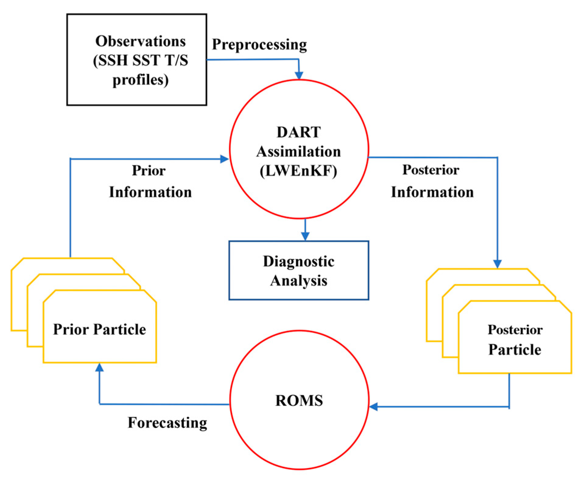
After assimilating all observations sequentially, the kernel density distribution mapping (KDDM) method is employed to adjust the probability density and optimize the performance of posterior particle ${\mathit{x}}_{i,k}^a$. Relevant procedures are elaborated in Appendix A. Notably, the LWEnKF data assimilation in this study is implemented within the framework of the ROMS-DART system, whose structure (including observation preprocessing, assimilation calculation, and ROMS forecasting links) is illustrated in Figure A1.

2.2.2. IEWVPS

The IEWVPS method incorporates IS4DVar as the proposal density into the particle smoother based on the IEWPF method. Implicit sampling is employed to sample in the high probability regions of posterior distribution, and all particles are ensured to have equal weights through an equal-weighting scheme. For more details about IEWVPS, refer to the article of Wang et al. (2020, 2021) [21,27]. In the IEWPF method, we use the proposal density $q\left(\mathit{\xi }\right)$ sampling of Gaussian distribution to replace the origin sampling $q\left({\mathit{x}}^n|{\mathit{x}}_i^{n-1},{\mathit{y}}^n\right)$. The relationship between the two can be expressed as follows:

$$q\left({\mathit{x}}^n|{\mathit{x}}_i^{n-1},{\mathit{y}}^n\right)={\displaystyle \frac{q\left(\mathit{\xi }\right)}{‖\mathit{J}‖}}$$

(6)

Here, $‖\mathit{J}‖$ represents the absolute value of the Jacobian matrix for the coordinate transform: $\mathbf{x}=g\left(\mathsf{\xi }\right)$. In the IEWVPS method, the transformation is defined as follows:

$${\mathbf{x}}_i^n={\mathbf{x}}_i^a+{\alpha }_i^{1/2}{\mathbf{P}}_i^{1/2}{\mathsf{\xi }}_i^n$$

(7)

where ${\mathbf{x}}_i^a$ represents the mode of proposal density $q\left({\mathit{x}}^n|{\mathit{x}}_i^{n-1},{\mathit{y}}^n\right)$, and ${\alpha }_i^{1/2}{\mathbf{P}}_i^{1/2}{\mathsf{\xi }}_i^n$ represents the equal-weight adjustment part. The mode of proposal density is obtained through minimizing the object function in IEWPF, which is similar to the process of minimizing cost functions in 4DVAR. Thus, a connection between 4DVAR and IEWPF can be established, which is precisely the concept behind IEWVPS. The assimilation process of IEWVPS differs from that of standard PF, so that it requires a specific time window for execution. Within this window $[1:n]$, the posterior probability density can be expressed using Bayes’ theorem:

$$p\left({\mathit{x}}^{0:n}|{\mathit{y}}^{1:n}\right)={\displaystyle \frac{p\left({\mathit{y}}^{1:n}|{\mathit{x}}^{0:n}\right)p\left({\mathit{x}}^{0:n}\right)}{p\left({\mathit{y}}^{1:n}\right)}}$$

(8)

With the introduction of the proposal density $q\left({\mathit{x}}_i^{0:n}|,{\mathit{y}}^{1:n}\right)$, it is possible to represent the weight of the particle as follows:

$$w_n={\displaystyle \frac{p\left({\mathit{y}}^{1:n}|{\mathit{x}}_i^{0:n}\right)}{p\left({\mathit{y}}^{1:n}\right)}}{\displaystyle \frac{p\left({\mathit{x}}_i^{0:n}\right)}{q\left({\mathit{x}}_i^{0:n}|{\mathit{y}}^{1:n}\right)}}$$

(9)

Here, the denominator can be expressed as the form of IS4DVAR:

$$p\left({\mathit{y}}^{1:n}|{\mathit{x}}_i^{0:n}\right)p\left({\mathit{x}}_i^{0:n}\right)\propto exp\left[J_i\left({\mathit{x}}_i^{0:n}\right)\right]$$

(10)

While $i=(1,\dots ,N_e)$ represents the number of particles, and $J_i\left({\mathit{x}}_i^{0:n}\right)$ represents the cost function for particle $i$. Then, combining the concept of implicit sampling, the status variable ${\mathbf{x}}_i^{a,0:n}$ of model can be described as follows:

$${\mathbf{x}}_i^{a,0:\mathrm{n}}={\mathbf{x}}_i^{4DVar,0:n}+{\alpha }_i^{1/2}{\mathbf{P}}_i^{1/2}{\mathsf{\xi }}_i^{0:n}$$

(11)

By implementing the IS4DVar method for each background particle ${\mathit{x}}_i^f$, we can obtain the vector ${\mathbf{x}}_i^{4DVar,0:n}$ within a given time window and cost function minima of the particle ${\displaystyle \frac{1}{2}}{\varphi }_i=min J_i$. The relevant literature provides detailed calculation steps for ROMS-4DVAR [5,6]. Then, we compute the implicit equal-weight parameter ${\alpha }_i$ by utilizing the Newton iteration method:

$$({\alpha }_i-1)({\mathsf{\xi }}_i^{0:n}{)}^{\mathrm{T}}{\mathsf{\xi }}_i^{0:n}-2\mathrm{l}\mathrm{o}\mathrm{g}{\alpha }_i^{N_x/2}-2\mathrm{l}\mathrm{o}\mathrm{g}\left(\left|1+{\displaystyle \frac{{\mathit{\xi }}_i^{0:n}}{{\alpha }_i^{1/2}}}{\displaystyle \frac{\partial {\alpha }_i^{1/2}}{\partial {\mathit{\xi }}_i^{0:n}}}\right|\right)=C-{\varphi }_i$$

(12)

where ${\mathsf{\xi }}_i^{0:n}$ represents a stochastic disturbance that conforms to the standard normal distribution, while $C$ denotes a constant term. The third step involves approximating the error covariance matrix $\mathbf{P}$ for posterior analysis in IS4DVar:

$${\mathbf{P}}^{1/2}\mathsf{\xi }={\mathbf{D}}^{1/2}\mathsf{\xi }\mathbf{V}(\mathbf{I}+{\mathbf{S}}^2{)}^{-1/2}$$

(13)

Here, ${\mathbf{D}}^{1/2}$ denotes the background error covariance matrix; $\mathbf{S}$ and $\mathbf{V}$ denote singular value vectors obtained by the singular value decomposition (SVD) of observation error covariance matrix ${\mathbf{R}}^{-1/2}$ and $\mathbf{G}{\mathbf{D}}^{1/2}$ ($\mathbf{G}$ represents the tangent linear model). The relevant calculation steps are elaborated in Appendix B.

2.3. ROMS Configuration

The Regional Ocean Model System (ROMS) is a free-surface, primitive-equation ocean numerical model widely used in regional ocean circulation and mesoscale process simulation. It adopts a finite-volume numerical scheme for horizontal discretization and a flexible S-coordinate vertical grid, which can effectively handle complex seabed topography and vertical stratification of seawater—the key advantages for simulating nonlinear mesoscale eddies in the northern South China Sea (SCS) [33].

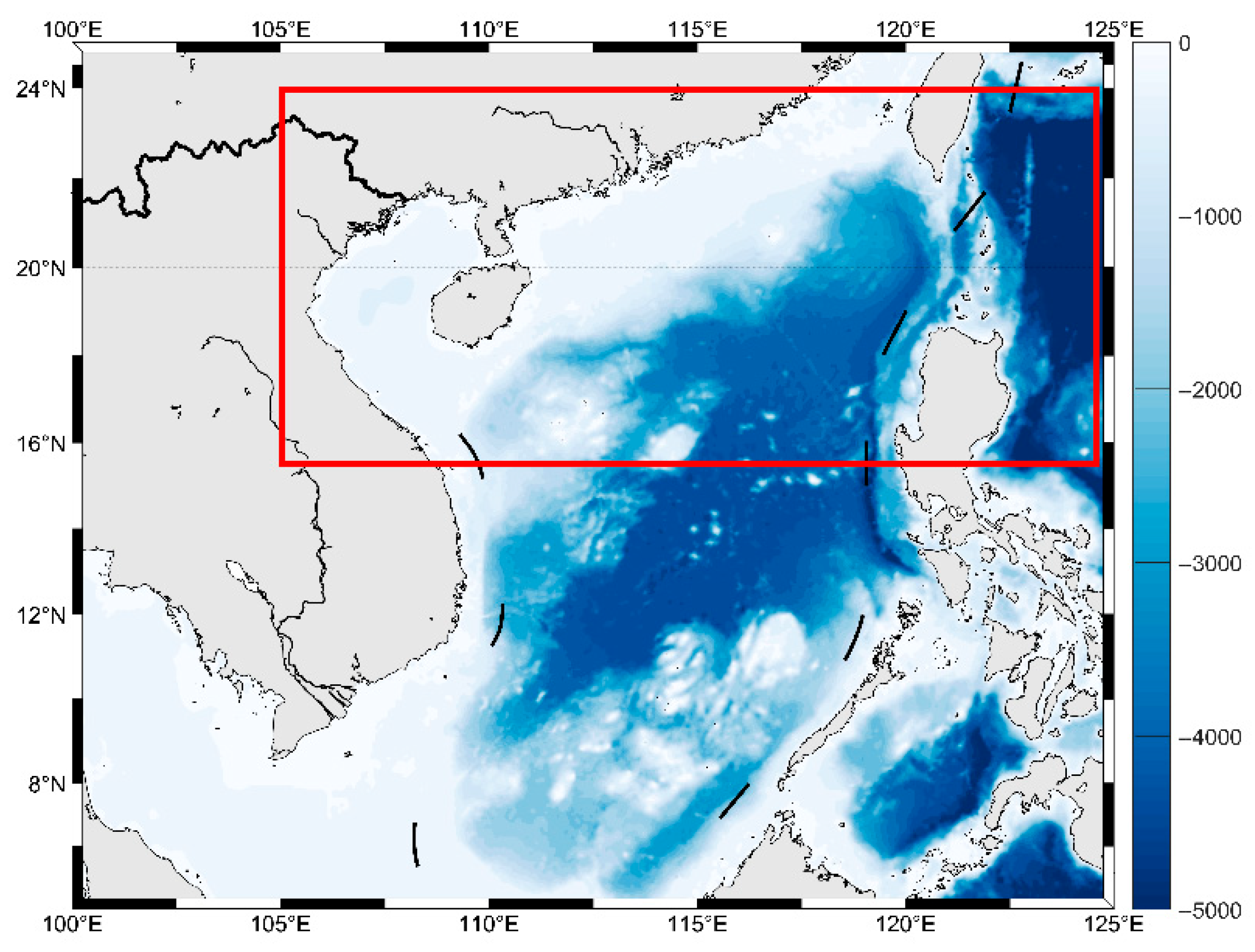
We investigate the northern region of the South China Sea, where large-scale wind-driven circulation exhibits distinct seasonal characteristics and features that are active in nonlinear mesoscale eddies. Furthermore, the complex topography of the seabed in this area presents challenges for assimilation systems. The simulated area depicted in Figure 1 covers a range of 15–24° N, 105–125° E, with the horizontal resolution of the model set to 1/6° × 1/6° and vertical direction divided into 24 layers. The time step used in the ROMS model is 60 s. The bathymetric data are derived from ETOPO2 with a 2′ × 2′ resolution. The initial and boundary conditions are obtained from the HYCOM reanalysis, which encompasses variables such as temperature, salinity, flow velocity, and sea surface height. The ERA-Interim reanalysis data provide the forcing conditions, including variables such as wind stress, net surface heat flux, net surface freshwater flux and shortwave radiation. Tides and river runoff are not considered in this study. We have chosen a significant mesoscale eddy that occurred in the SCS during July and August of 2017 as our research subject.

3. Assimilation Experiments

Although the design processes of LWEnKF and IEWVPS are different, they all achieve their operation through the assimilation cycle, with the concept of “assimilation window”. For the convenience of comparison, we set the assimilation window for both assimilation methods to 1 day. In a window, the assimilated observations include gridded SST and SLA observations at the middle time of the window and all the T/S profiles within ±2 days of the middle time. The total assimilation cycle is 61 days, from 1 July to 30 August 2017. For a better comparison, we set up the control (without assimilation), EnKF and IS4DVAR experiments. Every method has been tested in prior (background) and posterior (analysis) simulation experiments. The other settings for the five assimilation tests are consistent with those in Section 2.3.

The initial ensemble comprises the primary physical quantity information that governs state evolution, which holds significant importance in accelerating convergence to the true ocean state and enhancing filter performance during assimilation’s initial stage [34]. Initially, the model undergoes an 11-year integration (2007–2017) without assimilating the observed data. Subsequently, a principal component analysis with the empirical orthogonal function (EOF) of the following decade’s data is conducted to extract the salient features of oceanic conditions. The ultimate initial ensemble is generated via an exact second-order sampling scheme:

$${\mathbf{x}}_0^{\mathit{i}}=\mathbf{x}+\sqrt{N}{L}_0{\sigma }_i^T, i=1, \dots , N$$

(14)

In the aforementioned equation, $\mathbf{x}$ is derived from the patterns in the long-term results of the state on 1 July 2017. $N$ represents the number of ensemble members; $L_0$ represents a $N_x\times (N-1)$ sample matrix, which is composed of EOF principal components.${ \sigma }_i$ represents the row of a random matrix, which has a dimension of $N\times (N-1)$ with orthogonal columns and a sum equal to zero. This method for generating initial ensemble has been widely used in ocean data assimilation [35]. Through the assimilation cycle, initialization not only improves the following forecast, but also advances the whole data assimilation and prediction quality. LWEnKF, IEWVPS, and EnKF all employ 40 ensembles, whereas IS4DVAR does not require ensemble and adopts the mean of the ensemble as the initial background field.

3.1. Comparison of Surface States

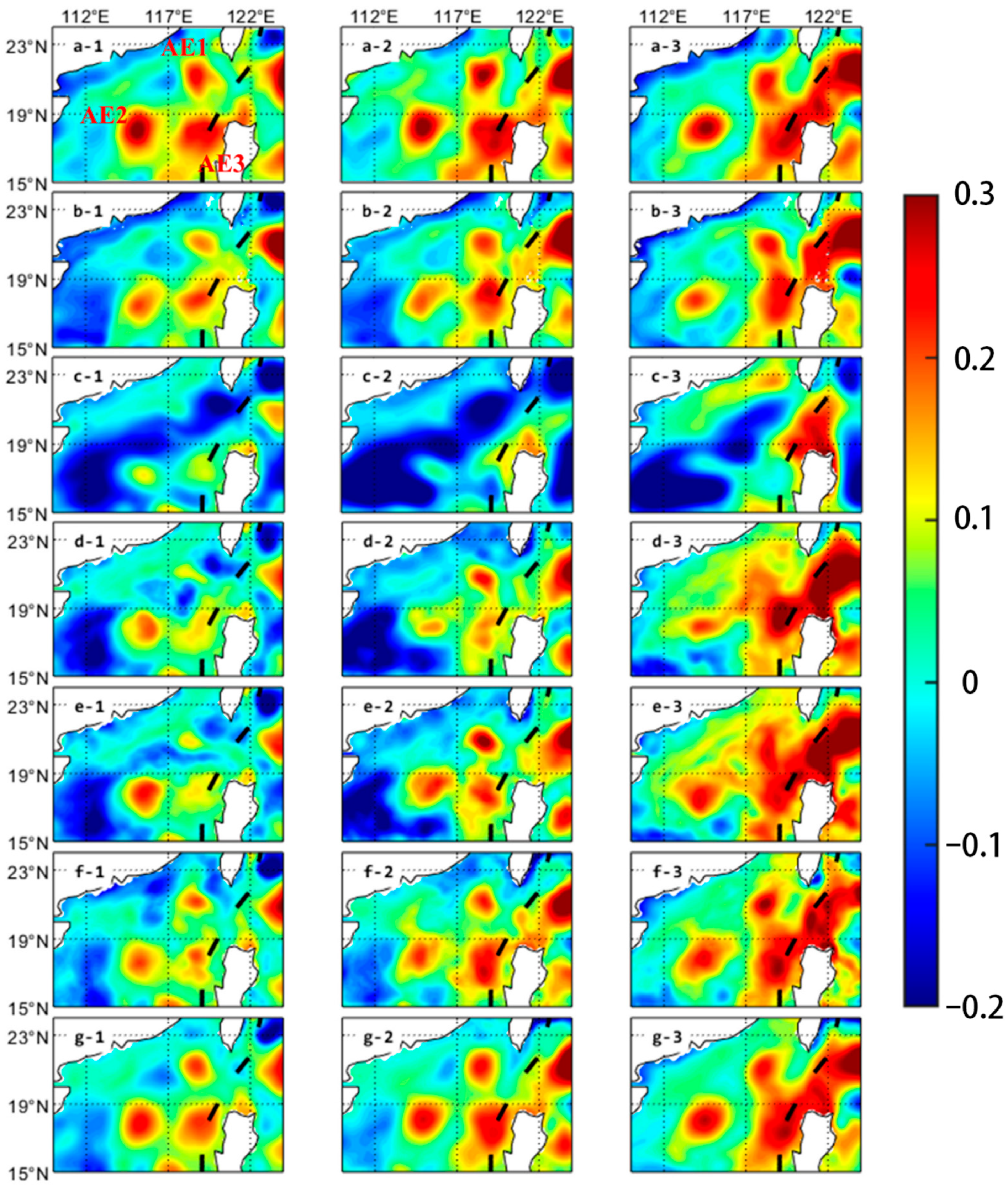
Three groups of 1-day forecasting results (on 14 July, 24 July and 3 August 2017) are shown in Figure 2 and Figure 3. There are three significant anticyclonic mesoscale eddies in the east and south of the simulated area, which can be seen from the SLA of AVISO data (Figure 2a). From 14 July to 3 August, the anticyclonic eddy in the east (marked as AE1 and AE3) has undergone periodical strong and weak changes; while the other eddy in the middle (AE2) remains relatively stable, with the strength and position changing slightly (the red rectangle in Figure 2(a-1)). There are significant differences between the control experiment and AVISO data, which indicate the substantial deviation from the real ocean surface states. Similarly, obvious differences exist among different types of DA methods. Although there are eddies observable in the target regions by EnKF, their shapes and intensities are significantly different from the AVISO data. By contrast, LWEnKF outperforms EnKF, but the forecast error is still large for AE1 among its results. Positions and shapes of the eddies predicted by IS4DVAR are in good agreement with AVISO as a whole, even if AE1’s strength is weaker than that observed. IEWVPS achieves the best results, whether in eddies or in the other regions.

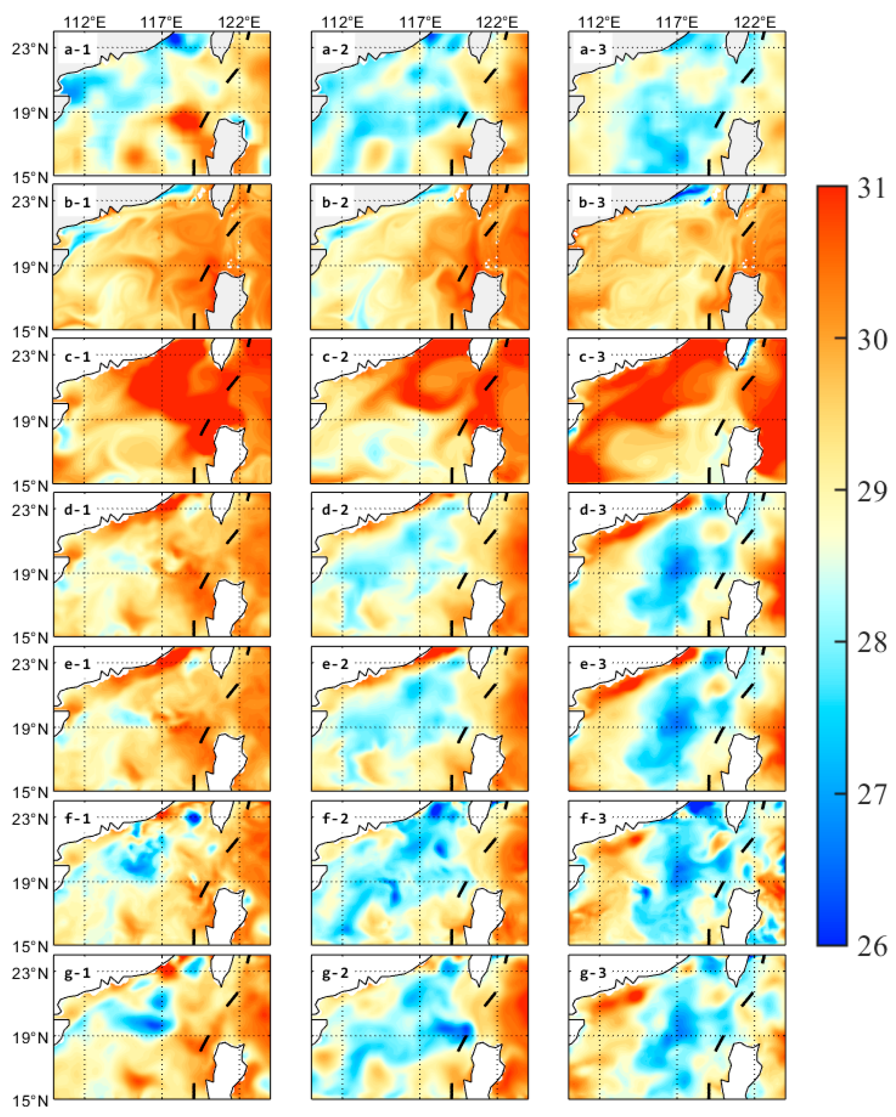
Figure 3 shows the SST from the observation and model data. The result shows that the error of SST is significantly large both in the control experiment and reanalysis data. Especially for the control experiment, the SST is obviously higher over northern seas compared to that in AVHRR observations. The forecast results of EnKF and LWEnKF on 14 July are not ideal, with the predicted SST being generally higher than that of AVHRR. This is probably due to the longer adjustment time required for EnKF and LWEnKF assimilation, which cannot fully adjust in the early days. The effect of EnKF and LWEnKF tends to stand out over time. On 24 July and 3 August, forecasting results of the four assimilation tests match the AVHRR data well across most of the seas, and even better than the CMEMS reanalysis data. However, the predicted SST by Kalman filter methods is apparently higher in the northern coast. Next, we perform the quantitative calculation of the root-mean-squared error (RMSE) between simulated and true ones.

3.2. Statistics of RMSE

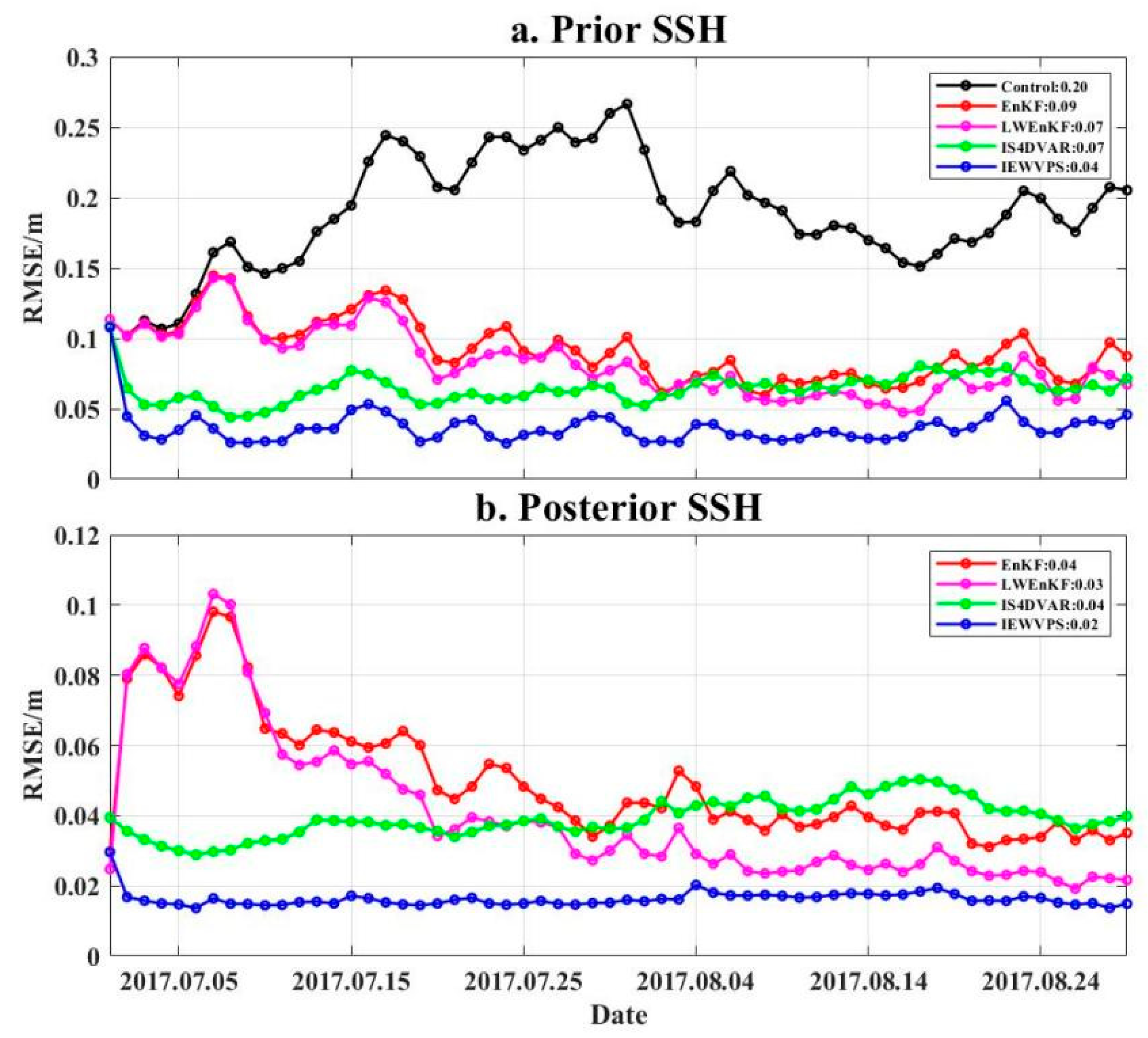
We calculate the RMSE of both prior (forecast) and posterior (analysis) results using spatial averaging at each analysis step. The time series and cumulative mean of RMSE are shown in Figure 4 (SLA) and Figure 5 (SST). The RMSE of prior SSH increases rapidly and deviates significantly from the true state of the ocean during the initial phase of the forecast. The RMSE of IS4Dvar and IEWVPS reaches a lower level after five assimilation windows, while it takes about 30 days for EnKF and LWEnKF to rank at the same level as that of IS4DVar. For the posterior results, the RMSE of IS4DVar shows an upward trend in the late assimilation period, which may be caused by the instability of the model. By the time of a long-running process, the advantages of EnKF and LWEnKF begin to emerge—the RMSE of EnKF and LWEnKF tends to be lower than that of IS4DVar after running for about 20 assimilation windows. Same as Section 3.1, the RMSE of IEWVPS is still the lowest of all assimilation experiments and remains stable throughout the whole simulation. In terms of cumulative mean value, compared with the control experiment, EnKF, LWEnKF, IS4DVar and IEWVPS reduce RMSE by 55%, 65%, 65% and 80%, respectively. Noteworthily, the RMSE of EnKF and LWEnKF shows a downward trend in the late assimilation period, and LWEnKF approaches the level of IEWVPS, which indicates that LWEnKF would have a better assimilation effect after the initial adjustment.

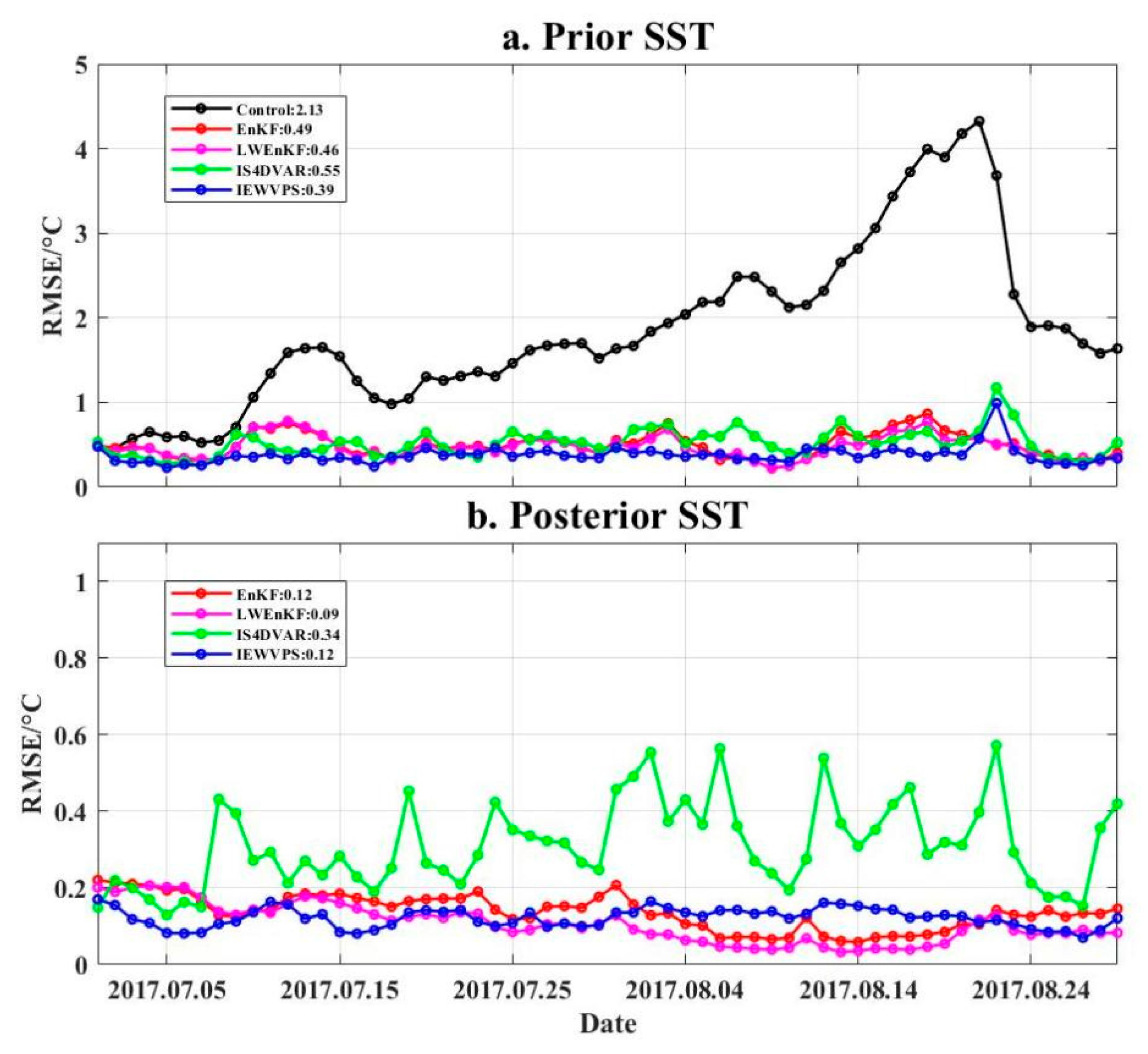
Figure 5 shows the RMSE for prior and posterior SST data. Same as the SSH, a spatial average is taken every day. There are no definite differences between control and assimilation experiments in the first 7 days, but the RMSE of control results continuously increases, seriously deviating from the real SST. In the prior results, the RMSE of the four assimilation experiments is relatively stable during the whole cycle, and the mean of IEWVPS is the lowest. The decrease in the RMSE is 77%, 78%, 74% and 82%, respectively, for the EnKF, LWEnKF, IS4DVar and IEWVPS methods. In the posterior results, IS4DVar is more volatile, which may be caused by the model’s uncertainty, and assimilation is not sufficient for effective adjustment. A month into the assimilation experiment, the RMSE of EnKF and LWEnKF is lower than that of IEWVPS; by the end of the cycle, the three methods are essentially the same. In general, LWEnKF has the lowest posterior RMSE by cumulation over the entire assimilation period.

4. Long-Term Forecasting

4.1. Results of Forecasting Surface States

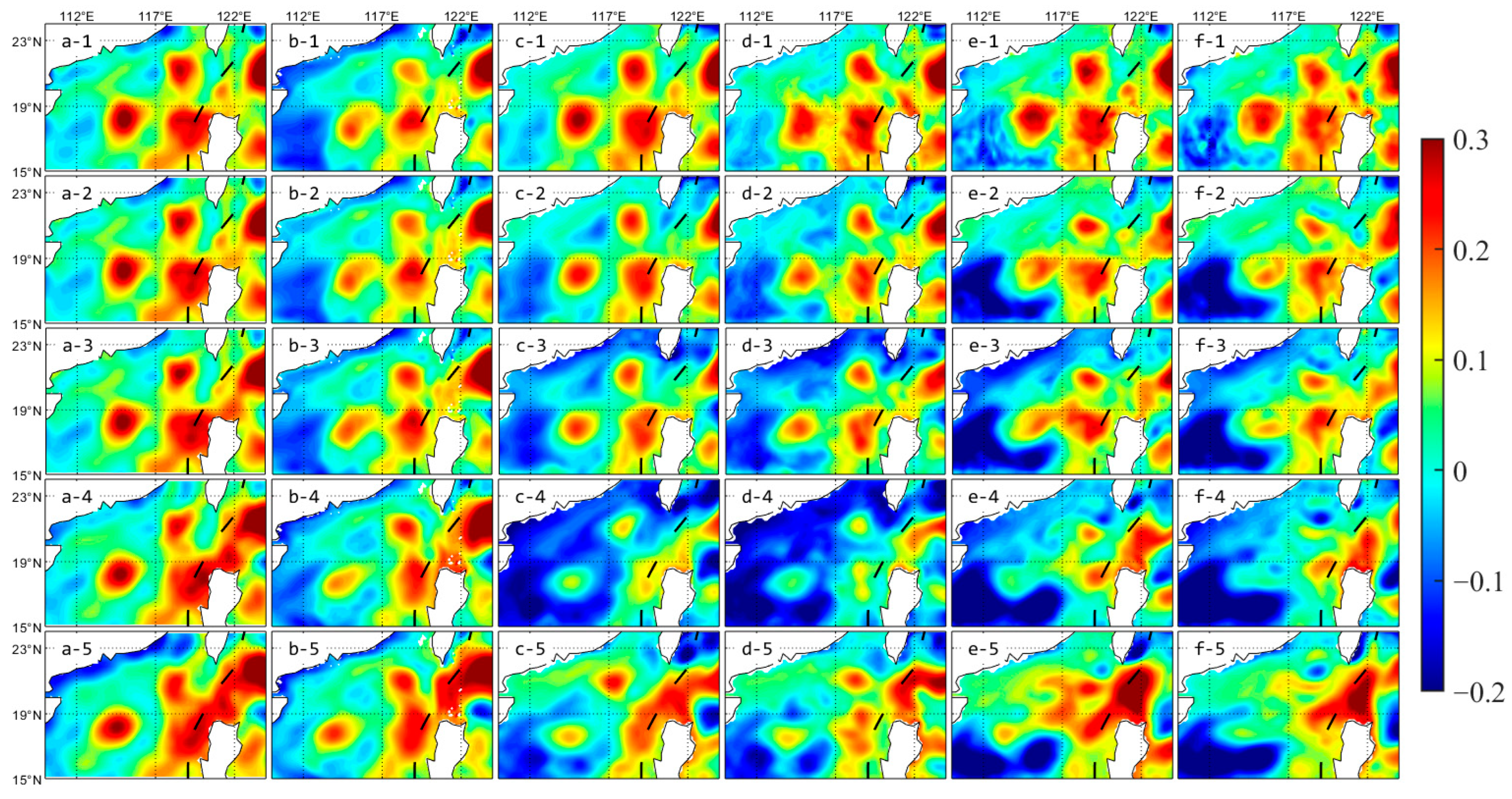
It can be seen from the 1-day assimilation window results of SLA (Figure 4) that the RMSE of EnKF and LWEnKF are roughly equal to IS4DVar after 20 July, which shows that the Kalman filter methods have completed the initial adjustment at this time. The posterior SSH of four experiments is also in good agreement with the AVISO data. Thus, the posterior analyses on 20 July are used as the initial fields for the 16-day forecasting experiments. Four groups of long-term forecasting results (on 20 July, 22 July, 25 July, 30 July and 4 August 2017) are shown in Figure 6. There are no significant differences in SLA in the initial fields among the four experiments, and the radius and amplitude of AE1 and AE2 are certainly consistent with the AVISO data.

On 22 July, the intensity of all forecasting mesoscale eddies is weaker than that of the AVISO data, but the result of IEWVPS is most consistent with the observation. The eddies predicted by the EnKF method are structurally different and become increasingly more significant in the subsequent results, making it difficult to identify the structure of AE1 and AE2. Longer forecast results (after 25 July) show that the overall distribution of SLA is already quite different from AVISO. On 30 July and 4 August, we are simply able to discern the features of mesoscale eddies only in IEWVPS and IS4DVar. In terms of the overall effect, 4DVar and its hybrid methods perform better than EnKF and its hybrid methods, with the best grade being of IEWVPS. Here, we present the CMEMS reanalysis as the control group, and the position of AE1 and AE2 is always identical to that of the AVISO data, notwithstanding that the intensity tends to be slightly weaker.

Afterwards, we will analyze the long-term forecasting results of SST (Figure 7). Compared with the initial field of SST on 20 July, the model simulation results are better than the reanalysis data, especially in the northwest region of SCS where SST is significantly cooler. Among them, the IEWVPS method is more accurate than others; there is a very obvious error of cold bias in SST within 19–21° N area among the IS4DVAR assimilation results, while EnKF and its hybrid methods have warm bias errors in the northern coastal shelf areas. As of 22 July, there has been a significant deviation between the forecasting SST and observational data. After five days of numerical simulation, LWEnKF and EnKF demonstrate significantly better performance in predicting the overall trend of SST compared to deterministic variational methods. Compared to SLA, SST has a much shorter predictability limit. Although the initial field generated by the IEWVPS method is optimal, EnKF and its hybrid methods are evidently more stable in long-term forecasting.

4.2. Statistics of Forecasting RMSE

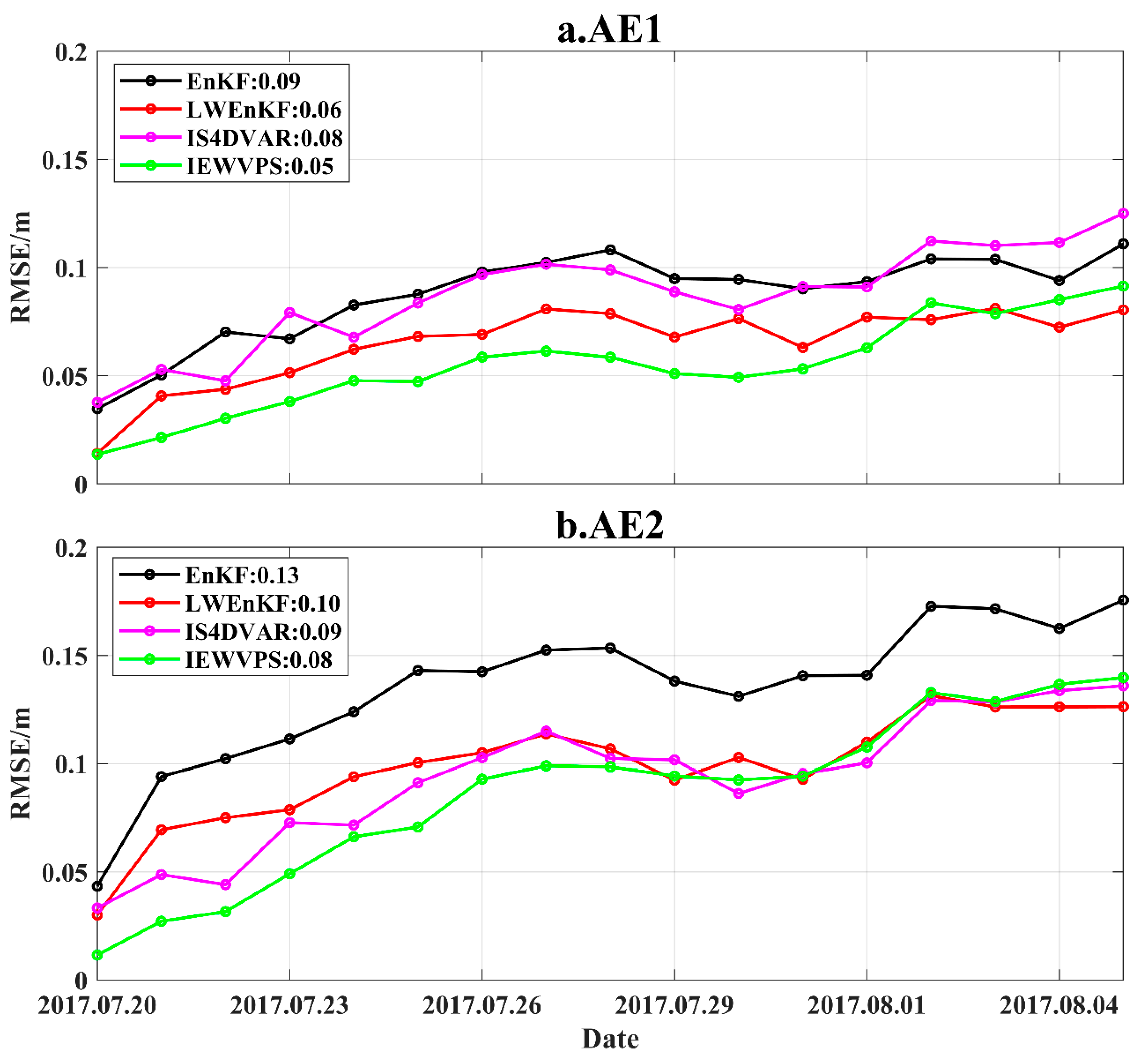
To quantitatively determine the forecasting effect, we calculate the RMSE of SLA in the general areas of AE1 and AE2 as well. The 16-day RMSE between forecasting SLA and true ones is shown in Figure 8. The RMSE for the four assimilation experiments increases as the forecasting time increases. The results show that IEWVPS is obviously superior to the other methods in the first 10 days (before 30 July); LWEnKF ranks second in the AE1 area, whereas it is slightly less well behaved than IS4DVar in the AE2 area. However, the situation changes gradually as the forecasting time prolongs, with the RMSE of LWEnKF falling below that of IEWVPS after 2 August. This is consistent with the conclusion of previous tests, which show that the Kalman filter methods may demand more time for adjustment. Although there are some differences between AE1 and AE2, LWEnKF exhibits outcomes similar to those of IS4DVar in the early stage, while its advantages become more apparent in the later stage, even outperforming IEWVPS.

4.3. Results of Undersea States

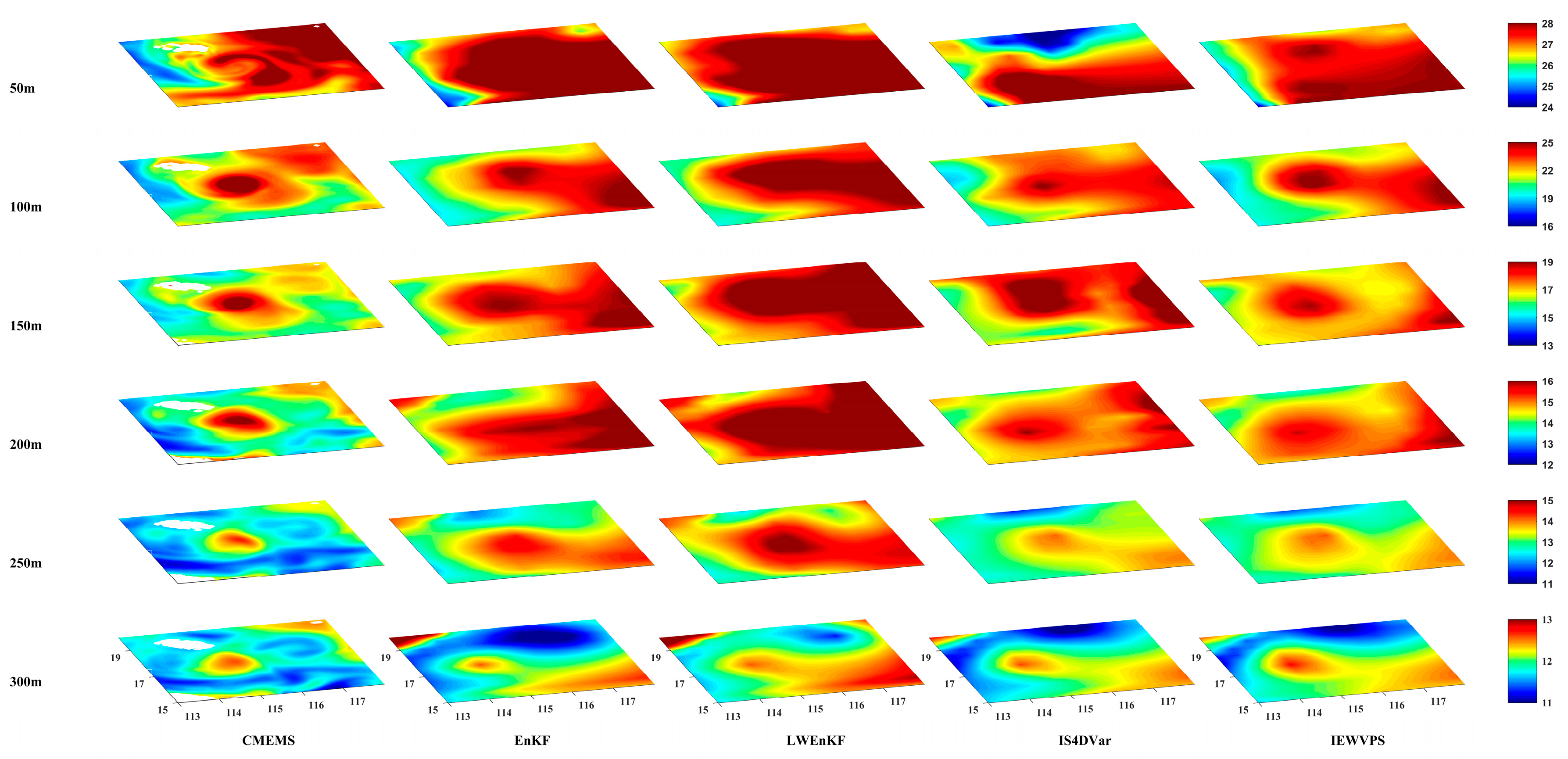
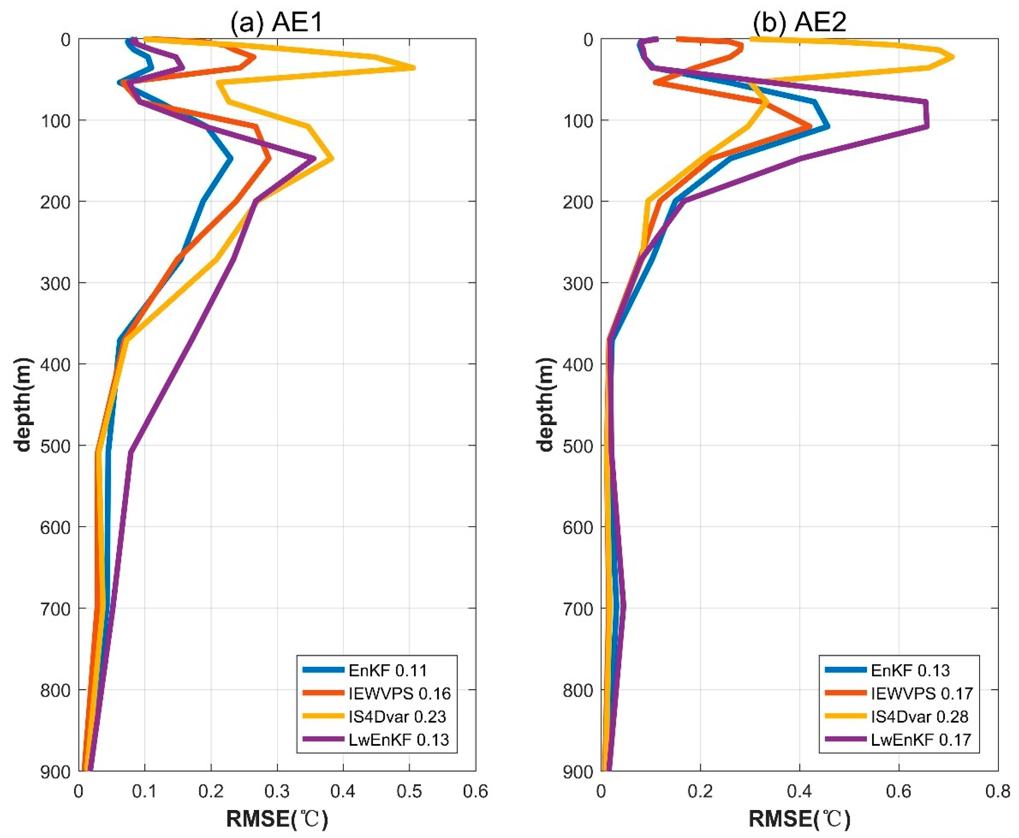
To assess the subaquatic structure of forecasting mesoscale eddies, we conducted a comparative analysis of undersea temperature (Figure 9) and the averaged 16-day forecast RMSE at every level (Figure 10), utilizing various DA methods. As of 25 July 2017, the surface structure of the mesoscale warm eddy remained relatively stable (refer to Figure 6). Therefore, temperature fields at various depths within the AE2 warm eddy region (15–20° N, 113–118° E) are extracted for comparison purposes (Figure 9), allowing for a clear observation of the three-dimensional structure of this mesoscale eddy. In the CMEMS reanalysis data results (the leftmost column in Figure 9), it is evident that the warm eddy’s high-temperature region shifts westward as depth increases, while its center gradually moves towards the same direction. Furthermore, the vertical structure of this warm eddy tends to tilt from top to bottom and aligns with its movement direction. Zhang et al. (2016) suggests that mesoscale eddies in the SCS may exhibit similar characteristics [36]. Due to the Beta-blockade Effect of topography, mesoscale eddies in the northern SCS propagate westward along the continental slope. The deep mesoscale eddy signal precedes the upper mesoscale vortex signal. The temperature fields predicted by the ROMS model (columns 2–4 in Figure 9) also clearly depict a warm eddy structure. However, compared with the reanalysis data, the high-temperature region of the warm eddy in our predictions is larger and its center’s temperature remains inadequate.

In general, the difference between forecast results and reanalysis data is significant. Due to the relative scarcity of observation data in the northern SCS, it is difficult for us to construct a complete eddy structure based on the observed T/S profiles. Therefore, we can only compare different assimilation methods’ forecast results with the CMEMS reanalysis data. In the depth range of 50–200 m, there exists a significant disparity between the forecast results and CMEMS. The prognostic results obtained from EnKF and IEWVPS are relatively satisfactory, with mesoscale eddies’ three-dimensional configuration being more proximate to actuality. As per the RMSE of vertical thermohaline profile (Figure 10), consistency in findings is observed, i.e., the maximum RMSE value was observed within the depth range of 50–200 m; however, beyond this limit, it decreased rapidly and approached zero. This is primarily attributed to the profound alterations in the physical characteristics of seawater above the thermocline. In terms of average RMSE, both EnKF and IEWVPS exhibit significantly superior performance compared to the other two methods (especially near the thermocline), and exert a certain degree of control over temperature fluctuations beneath the ocean surface. The IS4DVar method exhibits the highest degree of error, particularly near the 50 m depth. Noteworthily, the RMSE value in all tests indicates the highest error near the thermocline (100–200 m), suggesting that simulation errors of physical characteristics at this depth are the most significant. Although the DA methods can significantly enhance sea surface simulations, their impact on the thermocline region remains limited. In addition, the scarcity of T/S profile observation data in the northern SCS results in significant deviations below the sea surface during assimilation due to insufficient available data.

5. Computational Cost

When applying each assimilation method to actual services, it is necessary to evaluate not only its effectiveness but also its computational resource consumption. This section provides a comprehensive assessment of the computational costs associated with IEWVPS, IS4DVA, LWEnKF, and EnKF. In the numerical simulation test, an assimilation window of 1 day is set; that is, it takes 1 day to complete one assimilation cycle. In Section 2.2.1, we presented the computational procedure of LWEnKF, whose computational cost mainly arises from the nonlinear model integration, proposal density stage that uses EnKF to assimilate the observation, calculate proposal and likelihood weights, update model variables in the merge step and perform KDDM correction for high-order moments. The main cost of IEWVPS is attributed to the 4D-PSAS and particle equal-weight adjustment. Specifically, the cost of 4D-PSAS arises from nonlinear, tangent and adjoint mode integrals. Moore et al. (2011a, b) presented the computational procedures of IS4DVAR and 4D-PSAS, both of which involve outer and inner loops [5,6]. The outer loop updates the model variables in a nonlinear mode, while the inner loop minimizes the cost function. In this experiment, 4D-PSAS in IS4DVAR and IEWVPS requires 1 outer loop and 30 inner loops within a time window. Therefore, in each assimilation cycle of IEWVPS, each particle undergoes 2 nonlinear model integrations for 4D-PSAS, 30 linear tangent model integrations and 31 adjoint model integrations. The weight adjustment component necessitates an additional nonlinear and linear model integral, as well as invoking MATLAB(R2021a) external for the calculation of ${\alpha }_i$ and ${\mathbf{P}}^{1/2}\mathsf{\xi }$. The IS4DVAR solves in the primal space, requiring 2 nonlinear model integrations and 30 tangent linear and adjoint model integrations per assimilation cycle. In contrast, LWEnKF and EnKF do not require nonlinear, tangent linear and adjoint model integration, but have $2N_y$ and $N_y$ cycles to sequentially process observations per assimilation cycle. Additionally, the localization radius has a significant impact on computational costs. The EnKF method employs a local parameter $\mathit{c}$ of 0.02, and during the LWEnKF assimilation, the parameter $\mathit{c}$ in the EnKF step can also be set to 0.02.

The computational time of one complete assimilation cycle for IEWVPS, IS4DVA, LWEnKF and EnKF is statistically analyzed in

Table 1. Computational time consumed by different DA methods (IEWVPS, IS4DVA, LWEnKF and EnKF) during one assimilation cycle.

DA Method	IS4DVar	EnKF	LWEnKF	IEWVPS
Time (unit: s)	1113	7 + 15 = 22	7 + 17 = 24	858 + 49 = 907
Description		The average cost of nonlinear mode integration per day is 7 s, while for updating mode variables, it is 15 s.	The average cost of nonlinear mode integration per day is 7 s, while for updating mode variables, it is 17 s.	The average cost of each particle’s 4D-PSAS process is 858 s, while for weight adjustment at every step, it is 49 s.

. The testing hardware is an Intel Xeon CPU with 16 cores per node and 64 GB memory; a single particle is calculated in parallel using one node; the number of assimilated observations in each cycle is 3649. The statistical results indicate that the computational costs of Kalman filter methods are significantly lower than those of variational methods. In comparison with EnKF, an assimilation cycle in LWEnKF only takes 2 s longer. On the other hand, IEWVPS consumes approximately 20% less computing resources than IS4DVar. Noteworthily, the computational expense of an assimilation cycle in IEWVPS is approximately 38 times greater than that of LWEnKF. However, as the assimilation window length and mode resolution continue to increase, the computational cost of IEWVPS rises exponentially. In contrast, after a period of adjustment, LWEnKF can essentially achieve comparable assimilation effects to those of IEWVPS while maintaining significantly lower computational costs than both the IEWVPS and 4DVar methods, thus demonstrating strong potential for commercial applications. In general, the hybrid DA methods do not significantly increase computational costs compared to the traditional linear DA methods. Given its evident improvement in simulation accuracy, this approach holds great potential for future practical applications.

6. Discussion and Conclusion

DA is the foundation of ocean numerical prediction and reanalysis. While traditional methods such as EnKF, PF and 4DVAR have their own merits, they are inherently flawed in strong nonlinear systems. This study examines two novel hybrid DA techniques—LWEnKF and IEWVPS. Through theoretical integration, these new methods combine diverse assimilation benefits, thereby circumventing the assumption of model linearity and Gaussian error distribution. However, further verification is required to assess the applicability of hybrid DA methods in high-dimensional numerical models. Therefore, utilizing the ROMS-DART and ROMS-4DVAR assimilation systems with support from the regional ocean model ROMS, numerical simulation experiments are conducted in the northern SCS. The experiments are conducted over a two-month period, spanning from 1 July to 31 August 2017. Within the simulation region, two mesoscale eddies (AE1 and AE2) are consistently present. By comparing the effects of various assimilation methods on these eddies, the effectiveness of hybrid DA is evaluated. Furthermore, due to the complex topography of the northern shelf in the SCS and the abundant nonlinear seawater motion, this study can also test the stability of our assimilation system.

In the numerical simulation process spanning two consecutive months (with an assimilation window of 1 day), all four assimilation methods exhibit a relatively stable operation. Two measurement indices, namely SSH and SST, are selected to calculate the RMSE value between the simulation results (prior and posterior) and actual observed data. SST: Overall, both EnKF and LWEnKF deviate to some extent from the true ocean state (i.e., with larger RMSE values) in the early stages of the experiment. However, after approximately 20–30 assimilation cycles, the advantages of the Kalman filter gradually become apparent. At the advanced stage, the efficacy of EnKF and LWEnKF approaches that of IS4DVar and IEWVPS. LWEnKF outperforms EnKF, which underscores the benefits of PF combined with local weighting. In contrast, 4DVar-based methods exhibit less stability than EnKF-based methods and yield posterior results with significant RMSE fluctuations. Nonetheless, the IEWVPS method demonstrates superior performance compared to other methods throughout the simulation process and facilitates a smooth assimilation process. SSH: The analysis results based on SSH are essentially consistent with those of SST. In the early stages, the performance of the Kalman filter is inferior to that of the variational method. However, LWEnKF and IEWVPS exhibit similar behavior in later assimilation stages. Overall, the hybrid DA methods outperform the traditional assimilation methods in this test.

Based on the aforementioned research, we conduct a test on the long-term forecasting effect of mesoscale eddies. The initial fields are generated using the posterior data from four assimilation methods, and predictions are made for 16 consecutive days without further assimilation of observations. By comparing the distribution characteristics of eddies and the statistical RMSE, significant differences in prediction outcomes obtained from various initial fields are observed. After 5 days of model integration, the prediction results based on EnKF and LWEnKF initial fields indicate significant differences in mesoscale eddies’ morphology compared to actual observations. By the 10th day, it becomes difficult to discern the presence of eddies. In contrast, the 4DVar-based methods outperform the EnKF-based methods and can still identify mesoscale eddies’ characteristics by the 16th day. In addition, we also evaluate the forecasting of undersea temperature by different DA methods. The largest error occurs near the thermocline depth (50–200 m), which is also the depth where oceanic physical properties change most dramatically. In comparison, EnKF performs best in predicting underwater temperature, followed by IEWVPS and LWEnKF, while IS4Dvar shows the poorest performance. This may be related to the scarcity of T/S profile observation data in the northern SCS.

From the current development status of marine numerical models in various countries around the world, it is evident that the stability and computational complexity of 4DVAR and EnKF are significantly superior to those of the PF method. However, in the future, as the resolution of numerical models continues to increase, especially for the in-depth study of sub-mesoscale ocean processes, the advantages of the PF method will gradually become apparent. In addition, this study focuses on two warm eddies located in the northern part of the SCS, and further research is required to simulate the effect of cold ones. Obtaining more profile data within the mesoscale eddies’ region for comparison with model results would be beneficial in enhancing conclusion reliability. There is currently no definitive conclusion regarding the impact of these two mixed data assimilation methods on mesoscale eddy current fields, necessitating further verification. Furthermore, it is imperative to investigate the efficacy of mixed data assimilation techniques in high-resolution models. The particle filter framework for data assimilation offers the advantage of dispensing with the assumption of linear and Gaussian distribution, but its efficacy may not be fully demonstrated in simulating large-scale ocean phenomena characterized by weak nonlinear systems.

References

1. Wunsch, C. The Ocean Circulation Inverse Problem; Cambridge University Press: Cambridge, UK, 1996. [Google Scholar]
2. Bennett, A.F. Inverse Modeling of the Ocean and Atmosphere; Cambridge University Press: Cambridge, UK, 2007. [Google Scholar]
3. Edwards, C.A.; Moore, A.M.; Hoteit, I.; Cornuelle, B.D. Regional ocean data assimilation. Annu. Rev. Mar. Sci. 2015, 7, 21–42. [Google Scholar] [CrossRef]
4. Fu, J.-C.; Su, M.-P.; Liu, W.-C.; Huang, W.-C.; Liu, H.-M. Water Level Forecasting Combining Machine Learning and Ensemble Kalman Filtering in the Danshui River System, Taiwan. Water 2024, 16, 3530. [Google Scholar] [CrossRef]
5. Moore, A.M.; Arango, H.G.; Broquet, G.; Powell, B.S.; Weaver, A.T.; Zavala-Garay, J. The Regional Ocean Modeling System (ROMS) 4-dimensional variational data assimilation systems: Part I–System overview and formulation. Prog. Oceanogr. 2011, 91, 34–49. [Google Scholar] [CrossRef]
6. Moore, A.M.; Arango, H.G.; Broquet, G.; Edwards, C.; Veneziani, M.; Powell, B.; Foley, D.; Doyle, J.D.; Costa, D.; Robinson, P. The Regional Ocean Modeling System (ROMS) 4-dimensional variational data assimilation systems: Part II–performance and application to the California Current System. Prog. Oceanogr. 2011, 91, 50–73. [Google Scholar] [CrossRef]
7. Moore, A.M.; Arango, H.G.; Broquet, G.; Edwards, C.; Veneziani, M.; Powell, B.; Foley, D.; Doyle, J.D.; Costa, D.; Robinson, P. The Regional Ocean Modeling System (ROMS) 4-dimensional variational data assimilation systems: Part III–Observation impact and observation sensitivity in the California Current System. Prog. Oceanogr. 2011, 91, 74–94. [Google Scholar] [CrossRef]
8. Evensen, G. The ensemble Kalman filter: Theoretical formulation and practical implementation. Ocean. Dyn. 2003, 53, 343–367. [Google Scholar] [CrossRef]
9. Anderson, J.L. Localization and Sampling Error Correction in Ensemble Kalman Filter Data Assimilation. Mon. Weather. Rev. 2012, 140, 2359–2371. [Google Scholar] [CrossRef]
10. Houtekamer, P.L.; Zhang, F. Review of the ensemble Kalman filter for atmospheric data assimilation. Mon. Weather. Rev. 2016, 144, 4489–4532. [Google Scholar] [CrossRef]
11. Gordon, N.J.; Salmond, D.J.; Smith, A.F. Novel approach to nonlinear/non-Gaussian Bayesian state estimation. In Proceedings of the IEE Proceedings F (Radar and Signal Processing), London, UK, 20–22 April 1993; pp. 107–113. [Google Scholar]
12. Moradkhani, H.; Hsu, K.L.; Gupta, H.; Sorooshian, S. Uncertainty assessment of hydrologic model states and parameters: Sequential data assimilation using the particle filter. Water Resour. Res. 2005, 41. [Google Scholar] [CrossRef]
13. Hoteit, I.; Luo, X.; Bocquet, M.; Kohl, A.; Ait-El-Fquih, B. Data assimilation in oceanography: Current status and new directions. In New Frontiers in Operational Oceanography; Copernicus Publications: Katlenburg-Lindau, Germany, 2018; pp. 465–512. [Google Scholar]
14. Van Leeuwen, P.J.; Künsch, H.R.; Nerger, L.; Potthast, R.; Reich, S. Particle filters for high-dimensional geoscience applications: A review. Q. J. R. Meteorol. Soc. 2019, 145, 2335–2365. [Google Scholar] [CrossRef]
15. Papadakis, N. Assimilation de Données Images: Application au Suivi de Courbes et de Champs de Vecteurs. Ph.D. Thesis, Université Rennes 1, Rennes, France, 2007. [Google Scholar]
16. Poterjoy, J. A localized particle filter for high-dimensional nonlinear systems. Mon. Weather. Rev. 2016, 144, 59–76. [Google Scholar] [CrossRef]
17. Penny, S.G.; Miyoshi, T. A local particle filter for high-dimensional geophysical systems. Nonlinear Process. Geophys. 2016, 23, 391–405. [Google Scholar] [CrossRef]
18. Shen, Z.; Tang, Y. A modified ensemble Kalman particle filter for non-Gaussian systems with nonlinear measurement functions. J. Adv. Model. Earth Syst. 2015, 7, 50–66. [Google Scholar] [CrossRef]
19. Chen, Y.; Zhang, W.; Zhu, M. A localized weighted ensemble Kalman filter for high-dimensional systems. Q. J. R. Meteorol. Soc. 2020, 146, 438–453. [Google Scholar] [CrossRef]
20. Chen, Y.; Zhang, W.; Wang, P. An application of the localized weighted ensemble Kalman filter for ocean data assimilation. Q. J. R. Meteorol. Soc. 2020, 146, 3029–3047. [Google Scholar] [CrossRef]
21. Wang, P.; Zhu, M.; Chen, Y.; Zhang, W. Implicit equal-weights variational particle smoother. Atmosphere 2020, 11, 338. [Google Scholar] [CrossRef]
22. Courtier, P.; Thépaut, J.N.; Hollingsworth, A. A strategy for operational implementation of 4D-Var, using an incremental approach. Q. J. R. Meteorol. Soc. 1994, 120, 1367–1387. [Google Scholar] [CrossRef]
23. Zhu, M.; Van Leeuwen, P.J.; Amezcua, J. Implicit equal-weights particle filter. Q. J. R. Meteorol. Soc. 2016, 142, 1904–1919. [Google Scholar] [CrossRef]
24. Lorenz, E.N. Predictability: A problem partly solved. In Proceedings of the Seminar on Predictability; European Centre for Medium-Range Weather Forecasts (ECMWF): Reading, UK, 1996; pp. 1–18. [Google Scholar]
25. Shen, M.; Chen, Y.; Wang, P.; Zhang, W. Assimilating satellite SST/SSH and in-situ T/S profiles with the Localized Weighted Ensemble Kalman Filter. Acta Oceanol. Sin. 2022, 41, 26–40. [Google Scholar] [CrossRef]
26. Chen, Y.; Zhang, W.; Wang, H.; Cao, Y. Data assimilation system for the finite-volume community ocean model based on a localized weighted ensemble Kalman filter. J. Appl. Remote Sens. 2023, 17, 024508. [Google Scholar] [CrossRef]
27. Wang, P.; Zhu, M.; Chen, Y.; Zhang, W.; Yu, Y. Ocean satellite data assimilation using the implicit equal-weights variational particle smoother. Ocean. Model. 2021, 164, 101833. [Google Scholar] [CrossRef]
28. Chelton, D.B.; Schlax, M.G.; Samelson, R.M. Global observations of nonlinear mesoscale eddies. Prog. Oceanogr. 2011, 91, 167–216. [Google Scholar] [CrossRef]
29. Pearson, B.; Fox-Kemper, B.; Bachman, S.; Bryan, F. Evaluation of scale-aware subgrid mesoscale eddy models in a global eddy-rich model. Ocean. Model. 2017, 115, 42–58. [Google Scholar] [CrossRef]
30. Gao, S.; Wang, F.; Li, M.; Chen, Y.; Yan, C.; Zhu, J. Application of altimetry data assimilation on mesoscale eddies simulation. Sci. China Ser. D Earth Sci. 2008, 51, 142–151. [Google Scholar] [CrossRef]
31. Weiss, J.B.; Grooms, I. Assimilation of ocean sea-surface height observations of mesoscale eddies. Chaos Interdiscip. J. Nonlinear Sci. 2017, 27. [Google Scholar] [CrossRef] [PubMed]
32. Papadakis, N.; Mémin, É.; Cuzol, A.; Gengembre, N. Data assimilation with the weighted ensemble Kalman filter. Tellus A Dyn. Meteorol. Oceanogr. 2010, 62, 673–697. [Google Scholar] [CrossRef]
33. Shchepetkin, A.F.; Mcwilliams, J.C. The regional oceanic modeling system (ROMS): A split-explicit, free-surface, topography-following-coordinate oceanic model. Ocean. Model. 2005, 9, 347–404. [Google Scholar] [CrossRef]
34. Hoteit, I.; Pham, D.-T.; Triantafyllou, G.; Korres, G. A new approximate solution of the optimal nonlinear filter for data assimilation in meteorology and oceanography. Mon. Weather. Rev. 2008, 136, 317–334. [Google Scholar] [CrossRef]
35. Li, Y.; Toumi, R. A balanced Kalman filter ocean data assimilation system with application to the South Australian Sea. Ocean. Model. 2017, 116, 159–172. [Google Scholar] [CrossRef]
36. Zhang, Z.; Tian, J.; Qiu, B.; Zhao, W.; Chang, P.; Wu, D.; Wan, X. Observed 3D structure, generation, and dissipation of oceanic mesoscale eddies in the South China Sea. Sci. Rep. 2016, 6, 24349. [Google Scholar] [CrossRef]
37. Anderson, J.; Hoar, T.; Raeder, K.; Liu, H.; Collins, N.; Torn, R.; Avellano, A. The Data Assimilation Research Testbed: A Community Facility. Bull. Am. Meteorol. Soc. 2009, 90, 1283–1296. [Google Scholar] [CrossRef]
Figure 1. Simulation area (in a red box) and seabed topography of the SCS (unit: meter).
Atmosphere 16 01193 g001
Figure 2. The SLA (shading, unit: meter) of (a) AVISO data, (b) CMEMS reanalysis, (c) control, (d) EnKF, (e) LWEnKF, (f) 4DVAR and (g) IEWVPS posterior experiments. The columns represent the date for the predicted mesoscale eddies (on (1) 14 July, (2) 24 July and (3) 3 August 2017).
Atmosphere 16 01193 g002
Figure 3. The SST (shading, unit: °C) of (a) AVISO data, (b) CMEMS reanalysis, (c) control, (d) EnKF, (e) LWEnKF, (f) 4DVAR and (g) IEWVPS posterior experiments. The columns represent the date for the predicted mesoscale eddies (on (1) 14 July, (2) 24 July and (3) 3 August 2017).
Atmosphere 16 01193 g003
Figure 4. Spatially averaged RMSE of SSH at each analysis step for the control (black), EnKF (red), LWEnKF (purple), 4DVar (green) and IEWVPS (blue) experiments (from 1 July to 30 August 2017), computed with the (a) prior and (b) posterior data. The values in the right upper corner denote the time-averaged RMSE of different methods.
Atmosphere 16 01193 g004
Figure 5. The same as Figure 4 but for SST.
Atmosphere 16 01193 g005
Figure 6. The SLA (unit: meter) of (a) AVISO data, (b) CMEMS reanalysis, (c) IEWVPS, (d) IS4DVar, (e) LWEnKF and (f) EnKF forecasting experiments. The rows represent the date of the predicted mesoscale eddies (on (1) 20 July, (2) 22 July, (3) 25 July, (4) 30 July and (5) 4 August 2017).
Atmosphere 16 01193 g006
Figure 7. The SST (unit: °C) of (a) AVISO data, (b) CMEMS reanalysis, (c) IEWVPS, (d) IS4DVar, (e) LWEnKF and (f) EnKF forecasting experiments. The rows represent the date of the predicted mesoscale eddies (on (1) 20 July, (2) 22 July, (3) 25 July, (4) 30 July and (5) 4 August 2017).
Atmosphere 16 01193 g007
Figure 8. Spatially averaged RMSE of long-term forecasting SLA for the EnKF (black), LWEnKF (red), IS4DVar (purple) and IEWVPS (green) forecasting experiments (from 20 July to 5 August 2017), computed with the (a) AE1 and (b) AE2 areas. The values in the left upper corner denote the time-averaged RMSE of different methods.
Atmosphere 16 01193 g008
Figure 9. The forecasting undersea temperature of different DA methods on 25 July 2017. From left to right are CMEMS, EnKF, LWEnKF, IS4DVar and IEWVPS (unit: °C).
Atmosphere 16 01193 g009
Figure 10. Averaged 16-day forecast temperature RMSE at every level of (a) AE1 and (b) AE2, which is computed with the CMEMS data. The four profiles are of EnKF (blue line), LWEnKF (purple line), IS4DVar (yellow line) and IEWVPS (orange line). The values in the right bottom corner denote the vertical averaged RMSE of the four methods (unit: °C).
Atmosphere 16 01193 g010