PM_2.5 Concentration Prediction Model Utilizing GNSS-PWV and RF-LSTM Fusion Algorithms

Abstract

Inadequate screening of features and insufficient extraction of multi-source time-series data potentially result in insensitivity to historical noise and poor extraction of features for PM_2.5 concentration prediction models. Precipitable water vapor (PWV) data obtained from the Global Navigation Satellite System (GNSS), along with air quality and meteorological data collected in Suzhou city from February 2021 to July 2023, were employed in this study. The Spearman correlation analysis and Random Forest (RF) feature importance assessment were used to select key input features, including PWV, PM₁₀, O₃, atmospheric pressure, temperature, and wind speed. Based on RF, Long Short-Term Memory (LSTM), and Multilayer Perceptron (MLP) algorithms, four PM_2.5 concentration prediction models were developed using sliding window and fusion algorithms. Experimental results show that the root mean square error (RMSE) of the 1 h PM_2.5 concentration prediction model using the RF-LSTM fusion algorithm is 4.36 $\mathsf{\mu }\mathrm{g}/{\mathrm{m}}^3$, while its mean absolute error (MAE) and mean absolute percentage error (MAPE) values are 2.63 $\mathsf{\mu }\mathrm{g}/{\mathrm{m}}^3$ and 9.3%. Compared to the individual LSTM and MLP algorithms, the RMSE of the RF-LSTM PM_2.5 prediction model improves by 34.7% and 23.2%, respectively. Therefore, the RF-LSTM fusion algorithm significantly enhances the prediction accuracy of the 1 h PM_2.5 concentration model. As for the 2 h, 3 h, 6 h, 12 h, and 24 h PM_2.5 prediction models using the RF-LSTM fusion algorithm, their RMSEs are 5.6 $\mathsf{\mu }\mathrm{g}/{\mathrm{m}}^3$, 6.9 $\mathsf{\mu }\mathrm{g}/{\mathrm{m}}^3$, 9.9 $\mathsf{\mu }\mathrm{g}/{\mathrm{m}}^3$, 12.6 $\mathsf{\mu }\mathrm{g}/{\mathrm{m}}^3$, and 15.3 $\mathsf{\mu }\mathrm{g}/{\mathrm{m}}^3$, and their corresponding MAPEs are 13.8%, 18.3%, 28.3%, 38.2%, and 48.2%, respectively. Their prediction accuracy decreases with longer forecasting time, but they can effectively capture the fluctuation trends of future PM_2.5 concentrations. The RF-LSTM PM_2.5 prediction models are efficient and reliable for early warning systems in Suzhou city.

1. Introduction

Fine particulate matter (PM_2.5) is notable for its tiny size, high toxicity, and prolonged residence time in the air. It very easily penetrates the human respiratory system and is a significant threat to human health [1]. As a result, PM_2.5 pollution has become a global issue for environmental safety and public health [2]. In recent years, rapid industrialization and urbanization have led to a continuous increase in PM_2.5 concentration in many regions, such as the Beijing–Tianjin–Hebei region [3], Guangxi province [4], Nanjing city [5], and the Yangtze River Delta region [6] in China, as well as Isfahan [7] in Iran. These PM_2.5 incidents not only endanger local respiratory health but also decrease atmospheric visibility and increase the risk of traffic accidents. Therefore, accurate monitoring and forecasting of PM_2.5 concentration are crucial for environmental protection and public health [8].

The prediction methods of PM_2.5 concentration can be classified into mechanistic and data-driven models [9,10]. The mechanistic model utilizes atmospheric physicochemical equations to simulate the diffusion of pollutants and predict atmospheric motion. The Weather Research and Forecasting with Chemistry (WRF-Chem) model is one of the representative numerical prediction models [11]. However, it is challenging to fully understand the physical and chemical mechanisms of pollutants in complex atmospheric environments. Additionally, these models require high-accuracy emission inventories and complex parameterization [12], which result in high computational costs and limited real-time performance in practical applications. In contrast, data-driven models extract non-linear relationships from historical data using statistical and regression analysis methods. Data-driven models offer significant advantages in prediction efficiency, data adaptability, and parameter interpretability [13]. Traditional regression analysis, Support Vector Regression (SVR) [14], and Seasonal Autoregressive Integrated Moving Average (SARIMA) [15] algorithms have been widely applied to predict PM_2.5 concentration [16]. However, they are not effective at capturing the non-linearity of complex pollutants.

Machine learning algorithms significantly improve the prediction accuracy of models compared to traditional regression methods, so they have been widely used recently [17]. Random Forest (RF) effectively predicts outcomes by constructing multiple decision trees [18]. Ju reported that the root mean square error (RMSE) of predicted PM_2.5 concentration using RF in Nanjing was 5.68 $\mathsf{\mu }\mathrm{g}/{\mathrm{m}}^3$ [19]. Similarly, Guo et al. developed an RF-based PM_2.5 prediction model incorporating meteorological parameters from the Global Navigation Satellite System (GNSS), achieving notable performance in 6 h forecasting [20]. The Backpropagation Neural Network (BPNN) is capable of learning complex non-linear relationships [21], and the Extreme Gradient Boosting (XGBoost) algorithm achieves higher accuracy and efficiency by training multiple decision trees sequentially [22]. However, these traditional machine learning algorithms have difficulty extracting the periodicity of temporal data and cannot handle the dynamic cumulative effects of PM_2.5 effectively.

Deep learning algorithms effectively capture the periodic characteristics of temporal data, especially for Recurrent Neural Networks (RNNs). However, RNNs have problems of slow training and gradient explosion [23]. By introducing gating mechanisms, the Long Short-Term Memory (LSTM) neural network was developed to address these issues [24]. Kristiani et al. used air pollutant and meteorological data during 2017–2019 from 77 stations of the Taiwan Environmental Protection Administration to build PM_2.5 prediction models using RNN, LSTM, Convolutional Neural Network (CNN), Gated Recurrent Unit (GRU), and Bidirectional LSTM (Bi-LSTM) algorithms [25]. They found that the RMSE of the 1 h PM_2.5 prediction model using LSTM was 1.86 $\mathsf{\mu }\mathrm{g}/{\mathrm{m}}^3$, demonstrating superior performance for short-term forecasting. However, neglecting the spatial correlation of PM_2.5 atmospheric transport limits its prediction accuracy [26,27,28]. Therefore, Su et al. developed a PM_2.5 prediction model using CNN-LSTM fusion algorithms based on hourly atmospheric pollutants, meteorological parameters, and GNSS-derived precipitable water vapor (PWV) from 10 cities in the Beijing–Tianjin–Hebei region [29]. Its prediction RMSE was 7.55 $\mathsf{\mu }\mathrm{g}/{\mathrm{m}}^3$, representing a 26.23% improvement over BPNN and a 15.01% improvement over LSTM algorithms, indicating better spatiotemporal applicability. The fusion of LSTM and CNN algorithms for a PM_2.5 prediction model not only captures spatial features but also further improves the generalization ability and overall prediction accuracy by incorporating more mathematical algorithms.

Liu et al. developed a 24 h PM_2.5 prediction model using the LSTM and Fast Fourier Transform (FFT) fusion algorithm in the Beijing–Tianjin–Hebei region, integrating atmospheric pollutant data with ERA5 reanalysis data from the European Centre for Medium-Range Weather Forecasts (ECMWF). The FFT was used to extract periodic features. The RMSE of the model used in plain, mountainous, and plateau regions were 10.22 $\mathsf{\mu }\mathrm{g}/{\mathrm{m}}^3$, 8.56 $\mathsf{\mu }\mathrm{g}/{\mathrm{m}}^3$, and 9.02 $\mathsf{\mu }\mathrm{g}/{\mathrm{m}}^3$, respectively [30]. Wu et al. developed a PM_2.5 prediction model by integrating Complete Ensemble Empirical Mode Decomposition with Adaptive (CEEMDAN), Permutation Entropy (PE), Grey Wolf Optimizer (GWO), Variational Mode Decomposition (VMD), Mutual Information Function (MIF), Bidirectional LSTM (Bi-LSTM), and Attention Mechanism (AT) algorithms [31]. For Beijing, Wuhan, Urumqi, and Lhasa, the average RMSE, mean absolute error (MAE), mean absolute percentage error (MAPE), and R² of 1 h PM_2.5 prediction models were 1.5737 $\mathsf{\mu }\mathrm{g}/{\mathrm{m}}^3$, 1.3025 $\mathsf{\mu }\mathrm{g}/{\mathrm{m}}^3$, 5.18%, and 0.9961, respectively. Traditional mechanistic PM_2.5 prediction models like WRF-Chem face challenges of computational efficiency and high-accuracy emission inventories. As for data-driven approaches, traditional machine learning algorithms cannot easily capture the non-linearity and temporal dependencies of pollutants.

In recent years, the Yangtze River Delta region has experienced increased haze and PM_2.5 pollution [32]. To solve the above-mentioned problems, this study uses GNSS-PWV time series, air quality, and multi-source meteorological data collected at Suzhou city from February 2021 to July 2023. After a dual-stage feature selection using the Spearman correlation analysis and importance assessment using RF, key input variables are determined, including PWV, PM₁₀, O₃, atmospheric pressure, temperature, and wind speed. A new RF-LSTM fusion algorithm is applied to establish a PM_2.5 prediction model that supports PM_2.5 monitoring and environmental protection in Suzhou city. The model assumptions include atmospheric conditions remaining relatively stable within the prediction window, the relationship between input features and PM_2.5 concentration being learnable through machine learning algorithms, and the temporal patterns of the training data being representative of future conditions.

This paper is structured as follows. Section 2 describes the data and methodology. Section 3 describes the construction of the PM_2.5 concentration prediction model. Section 4 presents the results of the model’s prediction accuracy. Finally, the conclusion and future directions are outlined in Section 5.

2. Data and Methods

2.1. Data

Data from a GNSS station, an adjacent air quality monitoring station (1165A), and a meteorological station (58349) spanning from February 2021 to July 2023 in Suzhou city were collected, as illustrated in Figure 1. Their locations are in an urban area characterized by a dense population and high buildings. The GNSS station provided GNSS observations and meteorological variables (temperature and pressure). The ZTD was derived from GNSS data. It was also used to retrieve PWV. The air quality monitoring station, located approximately 1 km from the GNSS station, includes hourly SO₂, NO₂, CO, O₃, PM₁₀, and PM_2.5. The meteorological dataset encompassed wind direction, wind speed, precipitation, and relative humidity. The air quality and meteorological data were downloaded from the following website: https://q-weather.info (accessed on 25 October 2023).

2.2. Methods

2.2.1. PWV

(1)

GNSS-PWV

The International GNSS Service (IGS) offers free access to global data and products, including GNSS observations from reference stations, precise satellite orbit and clock products, and earth rotation parameters. To date, about 528 IGS stations have been established worldwide, with 17 of them located in China. In this study, GNSS data from the Suzhou station and six nearby IGS stations were processed using GAMIT 10.71 to obtain their zenith total delay (ZTD) at a 1 h resolution. The zenith hydrostatic delay (ZHD) was obtained from the Saastamoinen model, and the zenith wet delay (ZWD) was calculated by subtracting ZHD from ZTD. The ZWD was then converted to precipitable water vapor (PWV) using weighted mean temperature (T_m) [33]. The calculation formulas are as follows:

$$ZTD=ZHD+ZWD$$

(1)

$$ZHD={\displaystyle \frac{0.002768}{1-0.00266\times \mathit{cos}2\phi -0.00028\times h}}\times P_S$$

(2)

$$T_m={\displaystyle \frac{\int \frac{e}{T}dz}{\int \frac{e}{T^2}dz}}$$

(3)

$$PWV=ZWD\times {\displaystyle \frac{{10}^6}{{\rho }_w{R}_v\left(\frac{k_3}{T_m}+k_2^{\prime }\right)}}$$

(4)

where P_s is the surface pressure (hPa); φ is the station latitude (radian); h is the geodetic height (m); ${\rho }_w=1\times {10}^3 (\mathrm{k}\mathrm{g}/{\mathrm{m}}^3)$, is the density of water; $R_v=461.495 (\mathrm{J}\times {\mathrm{K}\mathrm{g}}^{-1}{\mathrm{K}}^{-1})$ is the specific gas constant for water vapor; and $k_2^{\mathrm{’}}=22.13\pm 2.20(\mathrm{K}/\mathrm{h}\mathrm{P}\mathrm{a})$ and $k_3=\left(3.739\pm 0.012\right)\times {10}^5 {(\mathrm{k}}^2/\mathrm{h}\mathrm{P}\mathrm{a})$ are constants of atmospheric refractivity.

(2)

RS-PWV

Radiosonde data was obtained from the University of Wyoming. Radiosonde is a widely used technique in meteorology for detecting water vapor. The atmospheric profile data is provided from the surface up to an altitude of approximately 30 km [34,35]. Radiosonde balloons are released twice or four times a day, recording geopotential height, temperature, pressure, wind speed, and wind direction at multiple atmospheric layers. These data can be used to retrieve the water vapor content at each level and the total column water vapor. Precipitable water vapor (PWV) can be calculated using the following formulas:

$$PWV={\displaystyle \frac{1}{{\rho }_W·g}}{\int }_{P_{top}}^{0}qdP$$

(5)

$$q=0.662{\displaystyle \frac{e}{p-0.378e}}$$

(6)

$$e=RH\ast e_s/100$$

(7)

$$e_s=6.112\times exp\left({\displaystyle \frac{17.67\times T}{T+243.5}}\right)$$

(8)

where ${\rho }_W=1\times {10}^3(\mathrm{k}\mathrm{g}/{\mathrm{m}}^3)$ is the density of water; P is the atmospheric pressure (hPa); $P_{top}$ is the pressure at the highest atmospheric layer; $g$ is the gravitational acceleration; q is the specific humidity ($\mathrm{g}/\mathrm{k}\mathrm{g}$); e is the actual water vapor pressure (hPa); $e_s$ is the saturation water vapor pressure (hPa); RH is the relative humidity at each layer (%); and T is the temperature at each layer (K).

2.2.2. Algorithms

(1)

Random Forest

RF is an ensemble learning algorithm. The model utilizes bagging [36], a technique that employs multiple random samples from the original dataset to train several decision trees. Furthermore, at the stage of node splitting for each decision tree, random features of the subset should be evaluated instead of the full feature dataset. The dual randomizations of data and features have been demonstrated to enhance model generalization and reduce the risk of overfitting [37].

The decision tree algorithm constructs a tree structure by recursively selecting the optimal feature. Maximizing information gain or minimizing the Gini index is commonly used to split the dataset [38]. Information gain reflects the entropy reduction of information before and after feature splitting. It is calculated as follows:

$$gain\left(D,v\right)=entropy\left(D\right)-\sum _{i=1}^n{\displaystyle \frac{\left|D_i\right|}{D}}entropy\left(D_i\right)$$

(9)

where $D$ is the current dataset, $v$ is a specific feature, $entropy\left(D\right)$ is the entropy of $D$, n is the number of subsets created by partitioning $D$ based on the feature v, and $D_i$ is the i-th subset.

The Gini index is a statistical measure of error probability in samples selected at random. A lower Gini index indicates a higher purity and better modelling performance of classification or regression analyses. It is calculated as follows.

$$gini\left(D,v\right)=\sum _{k=1}^d\sum _{k\ne m}{p}_k{p}_m=1-\sum _{k=1}^d{p}_k^2$$

(10)

where d is the total number of categories, and k and m represent the k-th and m-th categories. $p_m$ denotes the proportion of samples with feature ($v$) that belong to category m. $p_k$ denotes the proportion of samples with feature $\left(v\right)$ that belong to category k, ${\sum }_{k=1}^d{p}_k^2$ is the sum of the squared proportions for all categories k, and ${\sum }_{k\ne m}{p}_k{p}_m$ denotes the summation of $p_k{p}_m$ over all different categories.

Based on the feature importance analysis of RF, the key features of meteorological and pollutant factors are identified and used as inputs to the LSTM algorithm. This reduces input features, minimizes noise, improves training efficiency, and ultimately enhances prediction accuracy.

(2)

LSTM Neural Network

RNN is known for time-series prediction, but it often encounters problems of gradient vanishing and exploding. Hochreiter and Schmidhuber proposed the LSTM neural network [39], which effectively mitigates gradient problems and captures dependencies in long-term time-series data. The core components of an LSTM unit include the forget gate, input gate, cell state, and output gate. These gates utilize activation functions of sigmoid and tanh to decide on the selection or rejection of information, allowing the LSTM to effectively capture complex patterns in long sequences. The computational formulas of LSTM units are as follows:

$$f_t=\mathsf{\sigma }\left(W_f·\left[h_{t-1},x_t\right]+b_f\right)$$

(11)

$$i_t=\sigma \left(W_i·\left[h_{t-1},x_t\right]+b_i\right)$$

(12)

$${\tilde{C}}_t=tanh\left(W_c·\left[h_{t-1},x_t\right]+b_c\right)$$

(13)

$$C_t=f_t\ast C_{t-1}+i_t\ast {\tilde{C}}_{t-1}$$

(14)

$$o_t=\sigma \left(W_o·\left[h_{t-1},x_t\right]+b_o\right)$$

(15)

$$h_t=o_t\ast \mathrm{t}\mathrm{a}\mathrm{n}\mathrm{h}\left(C_t\right)$$

(16)

where $\sigma$ and $tanh$ represent the activation functions of sigmoid and tanh functions. $W_f,W_i,W_c,W_o$ are the weights for the respective gates, while $b_f,b_i,b_c,b_o$ are their corresponding bias vectors.$h_{t-1}$ is the hidden state from the previous (t − 1) step, and $x_t$ is the input at the current (t) step, including ZTD, PWV, temperature, PM₁₀, SO₂, PM_2.5, wind speed, and precipitation. $h_t$ represents the new hidden state. Figure 2 illustrates the structure diagram of LSTM cell units.

(3)

MLP

The Multilayer Perceptron (MLP) is a feedforward neural network that consists of an input layer, multiple hidden layers, and an output layer. In an MLP, the neurons in each layer are fully connected to all neurons in the next layer. The hidden layers employ non-linear activation functions to extract features from the input data. These extracted features are subsequently used for output prediction. Owing to the weight optimization via the backpropagation algorithm [40], the MLP is well suited for modeling non-linear relationships for PM_2.5 data.

2.2.3. Sliding Window

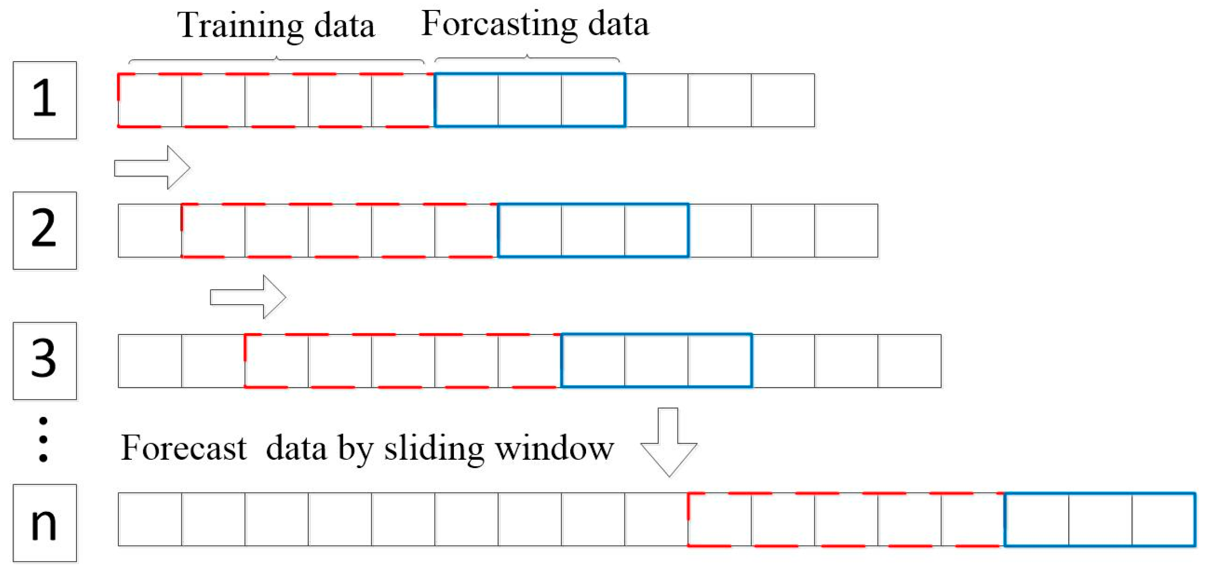
As shown in Figure 3, the sliding window is commonly used for processing and analyzing time-series data. First, the window width (W) of the training dataset and a prediction window width (S) are defined along the time axis. Next, the input features—ZTD, PWV, temperature, pressure, PM₁₀, CO, wind speed, and precipitation—within the interval [0, W] are used to predict the PM_2.5 concentration in the interval [W, W + S]. Subsequently, the window is continuously shifted along the time axis, utilizing features within [n, n + W] to predict the PM_2.5 concentration for [n + W, n + W + S]. This process is repeated until the end of the time series.

2.2.4. Accuracy Assessments

Bias, RMSE, MAE, and MAPE are used to evaluate the accuracy of the PM_2.5 concentration prediction models. The formulas are as follows:

$$Bias={\displaystyle \frac{1}{n}}{\sum }_{i=1}^n(y_i-{\widehat{y}}_i)$$

(17)

$$RMSE=\sqrt{{\displaystyle \frac{1}{n}}{\sum }_{i=1}^n{\left(y_i-{\widehat{y}}_i\right)}^2}$$

(18)

$$RMSE=\sqrt{{\displaystyle \frac{1}{n}}{\sum }_{i=1}^n{\left(y_i-{\widehat{y}}_i\right)}^2}$$

(19)

$$MAPE={\displaystyle \frac{100\mathrm{\%}}{n}}{\sum }_{i=1}^n\left|{\displaystyle \frac{y_i-{\widehat{y}}_i}{y_i}}\right|$$

(20)

where $y_i$ represents the truth or reference, ${\widehat{y}}_i$ is the predicted value, and n is the number of total samples.

3. Model Construction

3.1. Feature Selection

The Spearman correlation analysis was used to select the initial features.

Table 1. Correlation coefficients between PM_2.5 and atmospheric pollutants during 2021–2023.

Atmospheric Pollutants	SO2	NO	CO		O3		PM10
	0.317 **	0.477 **	0.508 **		−0.145 **		0.844 **
Meteorological Elements	ZTD	PWV	Temp	Pres	RH	WS	Rain
	−0.397 **	−0.395 **	−0.299 **	0.266 **	−0.039 **	−0.318 **	−0.171 **

** indicates significant correlation at the 0.01 level.

shows the correlations of meteorological factors (GNSS-PWV, ZTD, and wind speed) and atmospheric pollutants (SO₂, NO, and PM10) with PM_2.5. As shown in Table 1, PM_2.5 exhibited significant positive correlations with SO₂, NO₂, CO, and PM₁₀; their correlation coefficients were 0.317, 0.477, 0.508, and 0.844, respectively. Notably, the correlation coefficient between O₃ and PM_2.5 was −0.145, indicating a negative correlation. This may be attributed to the reaction of O₃ with water vapor in the air, promoting the production of PM_2.5, so the decrease in O₃ concentration may be accompanied by an increase in PM_2.5 concentration. PM_2.5 exhibited negative correlations with PWV, ZTD, temperature, humidity, wind speed, and precipitation; their coefficients were −0.397, −0.395, −0.299, −0.039, −0.318, and −0.171, respectively. In contrast, the positive correlation coefficient between atmospheric pressure and PM_2.5 was 0.226. Suzhou city is located in the Eastern China region, characterized by a temperate climate and abundant precipitation. The high level of ZTD and PWV often coincides with precipitation, which is a primary factor in reducing PM_2.5 concentration. Therefore, ZTD, PWV, and precipitation are negatively correlated with PM_2.5. When the temperature rises, the air expands and its density decreases. Then, the air pressure drops, enhancing atmospheric dispersion and promoting pollutant diffusion. Thus, temperature is correlated negatively with PM_2.5, and atmospheric pressure is correlated positively with PM_2.5. Furthermore, since PM_2.5 is easily transported by air currents, leading to pollutant dispersion, wind speed is negatively correlated with PM_2.5 concentration.

In summary, a few atmospheric pollutants and meteorological parameters show significant correlations with PM_2.5 concentration at the 0.01 level. They are regarded as the primary influencing factors of PM_2.5. However, since their correlation coefficients are relatively low, using these correlation coefficients directly as input variables may result in insufficient fitting and decreased prediction accuracy. Therefore, it is necessary to select input features using importance evaluation of RF, further improving its efficiency and prediction accuracy.

The RF algorithm is simple to implement, trains efficiently, and evaluates feature importance automatically. Therefore, the “feature_importances” in the “scikit-learn” library of the Python (V3.8.10) environment was used to evaluate the importance of each feature [41]. This evaluation primarily relies on out-of-bag (OOB) error estimation, which can accurately measure the contribution of each feature to modelling performance. Accordingly, after inputting the features screened by Spearman correlation analysis into the RF algorithm, the importance index of each feature for the PM_2.5 concentration prediction model can be obtained.

Table 2. The importance index of features on PM_2.5 concentration.

Feature	PM10	Pres	Temp	ZTD	O3	PWV	WS	RH	NO2	SO2	CO	Rain
Importance	0.113	0.102	0.09	0.098	0.097	0.097	0.094	0.09	0.09	0.057	0.045	0.013

presents the importance indexes of each feature. SO₂ and CO exhibited low importance (0.057 and 0.045) for PM_2.5 concentration and were thus excluded from feature selection. Although ZTD and PWV had similar importance indexes, PWV directly represents water vapor and has a clear physical association with PM_2.5. Therefore, ZTD was excluded as a feature as well. Although humidity exhibited a weak direct correlation with PM_2.5, it can indirectly regulate PM_2.5 by influencing aerosol hygroscopic growth. Similarly, the precipitation shows a relatively low importance index, but it can directly affect PM_2.5 concentration from the perspective of a physical mechanism. Consequently, PM₁₀, air pressure, temperature, O₃, PWV, wind speed, humidity, and NO₂ were selected as input features, and the output feature was true PM_2.5 to construct the PM_2.5 concentration prediction model using MLP, LSTM, RF-MLP, and RF-LSTM algorithms.

3.2. Data Normalization

To avoid disproportionately focusing on features with larger ranges during neural network training and to accelerate convergence and improve prediction accuracy, the min–max normalization was used to process PM_2.5 and other input data [42].

$$x={\displaystyle \frac{x-min}{max-min}}$$

(21)

3.3. Selection of Sliding Windows

The selection of an appropriate sliding window length is pivotal in this study, as shown in

Table 3. The PM_2.5 prediction accuracy of different sliding window lengths ($\mathsf{\mu }\mathrm{g}/{\mathrm{m}}^3$).

Window Length	RMSE	Bias
6 h	8.68	−0.78
12 h	7.30	1.04
24 h	6.88	−0.44
48 h	6.90	−0.88
72 h	6.85	0.36

. The window lengths mainly involved 6 h, 12 h, 24 h, 48 h, and 72 h. The RMSEs of 6 h, 12 h, 24 h, 48 h, and 72 h were 8.68 $\mathsf{\mu }\mathrm{g}/{\mathrm{m}}^3$, 7.30 $\mathsf{\mu }\mathrm{g}/{\mathrm{m}}^3$, 6.88 $\mathsf{\mu }\mathrm{g}/{\mathrm{m}}^3$, 6.90 $\mathsf{\mu }\mathrm{g}/{\mathrm{m}}^3$, and 6.85 $\mathsf{\mu }\mathrm{g}/{\mathrm{m}}^3$, respectively. The RMSEs of 24 h, 48 h, and 72 h were at the same level, indicating stable prediction accuracy after the window length reached 24 h or more. Therefore, the 24 h sliding window length was selected due to its reduced data amount and higher computational efficiency.

3.4. Model Construction

Next, PM_2.5 concentration prediction models using MLP, LSTM, RF-MLP, and RF-LSTM algorithms were constructed. For this, appropriate parameters were set for each algorithm.

The MLP consisted of two hidden layers with 50 neurons in each layer. Its activation function was set as “relu”. Its loss function was mean squared error (MSE), and the optimizer was “Adam”, with an initial learning rate of 0.01, a weight decay of 0.001, and 100 training epochs. The LSTM model employed a two-layer stacked architecture with 128 hidden units in each layer, and it did not utilize a bidirectional structure. The loss function, optimizer, learning rate, and weight decay of the proposed model were consistent with those employed in the MLP algorithm. The bidirectional LSTM (Bi-LSTM) was consistent with the parameters of LSTM.

For the RF-MLP and RF-LSTM fusion algorithms, the RF was used for feature selection; its tree number was set to 100, and the maximum depth was set to 10. Subsequently, the same neural network structures and parameter settings as those of the MLP and LSTM algorithms were applied for prediction. The detailed parameter settings of all algorithms are summarized in

Table 4. Parameter settings of MLP, LSTM, RF-MLP, Bi-LSTM and RF-LSTM algorithms.

Parameter Name	Settings (Fusion Algorithm Name)
Hidden Layer Dimension	50 (MLP, RF-MLP and Bi-LSTM)
Stacking Layers	2 (MLP, LSTM, Bi-LSTM, RF-MLP, and RF-LSTM)
Activation Function	rule (MLP and RF-MLP)
Bidirectional Option	0.2 (MLP, LSTM, Bi-LSTM, RF-MLP, and RF-LSTM)
Loss Function	MSE (MLP, LSTM, Bi-LSTM, RF-MLP, and RF-LSTM)
Learning Rate	0.01 (MLP, LSTM, Bi-LSTM, RF-MLP, and RF-LSTM)
Weight Decay Coefficient	0.001 (MLP, LSTM, Bi-LSTM, RF-MLP, and RF-LSTM)
Training Epochs	100 (MLP, LSTM, Bi-LSTM, RF-MLP, and RF-LSTM)
Hidden Layer Dimension	128 (LSTM, Bi-LSTM and RF-LSTM)
Bidirectional Option	False (LSTM and RF-LSTM)
Bidirectional Option	True (Bi-LSTM)
Random Forest	100 (RF-MLP and RF-LSTM)
Max Depth	10 (RF-MLP and RF-LSTM)

.

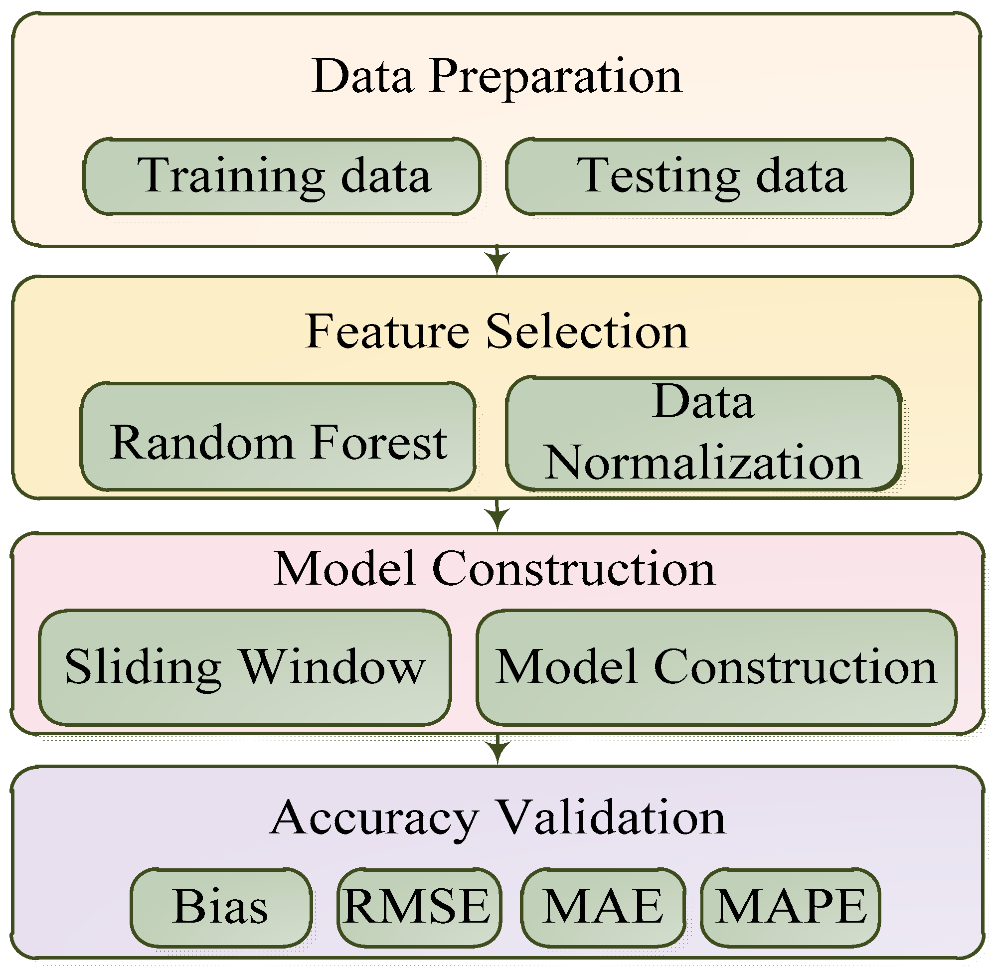
Figure 4 presents the workflow for constructing the PM_2.5 concentration prediction model using MLP, LSTM, Bi-LSTM, RF-MLP, and RF-LSTM neural networks. The specific steps were as follows: First, the data of SO₂, NO₂, CO, PM_2.5, PWV, ZTD, temperature, and relative humidity were collected from GNSS stations and environmental and meteorological monitoring stations. The data from February 2021 to December 2022 were used as the training dataset, with 80% used for training and the remaining 20% for cross-validation, while the data from January 2023 to July 2023 served as the testing dataset. Next, the RF algorithm was used for feature selection. Data normalization was conducted using the min–max method. Subsequently, the PM_2.5 concentration prediction model was constructed using MLP, LSTM, Bi-LSTM, RF-MLP, and RF-LSTM algorithms with a 24 h sliding window (width = 24). Finally, the prediction accuracy of MLP, LSTM, Bi-LSTM, RF-MLP, and RF-LSTM of PM_2.5 models was validated.

4. Result and Analysis

4.1. Accuracy of Models

Table 5. The accuracy of 1 h PM_2.5 prediction models using MLP, LSTM, Bi-LSTM, RF-MLP, and RF-LSTM algorithms $\left(\mathsf{\mu }\mathrm{g}/{\mathrm{m}}^3\right)$.

Algorithm	RMSE	Bias	MAE	MAPE (%)
LSTM	6.68	−0.44	4.96	17.70
Bi-LSTM	6.17	−4.18	4.47	16.35
MLP	5.68	1.72	4.00	16.80
RF-MLP	5.89	−0.21	3.98	14.90
RF-LSTM	4.36	−0.02	2.63	9.30

summarizes the prediction accuracy of 1 h PM_2.5 concentration models using MLP, LSTM, Bi-LSTM, RF-MLP, and RF-LSTM. As shown in Table 4, the RMSE of the 1 h PM_2.5 concentration model using RF-LSTM was 4.36 $\mathsf{\mu }\mathrm{g}/{\mathrm{m}}^3$, which was 34.7%, 29.3%, 23.2%, and 25.9% lower than that of LSTM, Bi-LSTM, MLP, and RF-MLP, respectively. The MAEs of 1 h PM_2.5 concentration models using RF-LSTM, LSTM, Bi-LSTM, MLP, and RF-MLP were 2.63 $\mathsf{\mu }\mathrm{g}/{\mathrm{m}}^3$, 4.96 $\mathsf{\mu }\mathrm{g}/{\mathrm{m}}^3$, 4.47 $\mathsf{\mu }\mathrm{g}/{\mathrm{m}}^3$, 4.00 $\mathsf{\mu }\mathrm{g}/{\mathrm{m}}^3$, and 3.98 $\mathsf{\mu }\mathrm{g}/{\mathrm{m}}^3,$ respectively. Furthermore, the bias of 1 h PM_2.5 concentration models using RF-LSTM was close to zero, indicating that there was almost no systematic deviation between the predicted and actual PM_2.5. The MAPE of 1 h PM_2.5 concentration models using RF-LSTM was 9.30%, which was also significantly lower than those models using other algorithms.

Figure 5 compares the 1 h predicted PM_2.5 concentration using RF-LSTM with the true value and its fitting plot. As shown in Figure 5a, the overall trend of the predicted and true PM_2.5 closely matches each other. Figure 5b displays a scatter between predicted PM_2.5 and truth. The regression line slope is close to 1, and the coefficient of determination (R²) is 0.977, indicating that the RF-LSTM algorithm provides reliable and accurate PM_2.5 concentration predictions.

4.2. Prediction Accuracy of the RF-LSTM Model

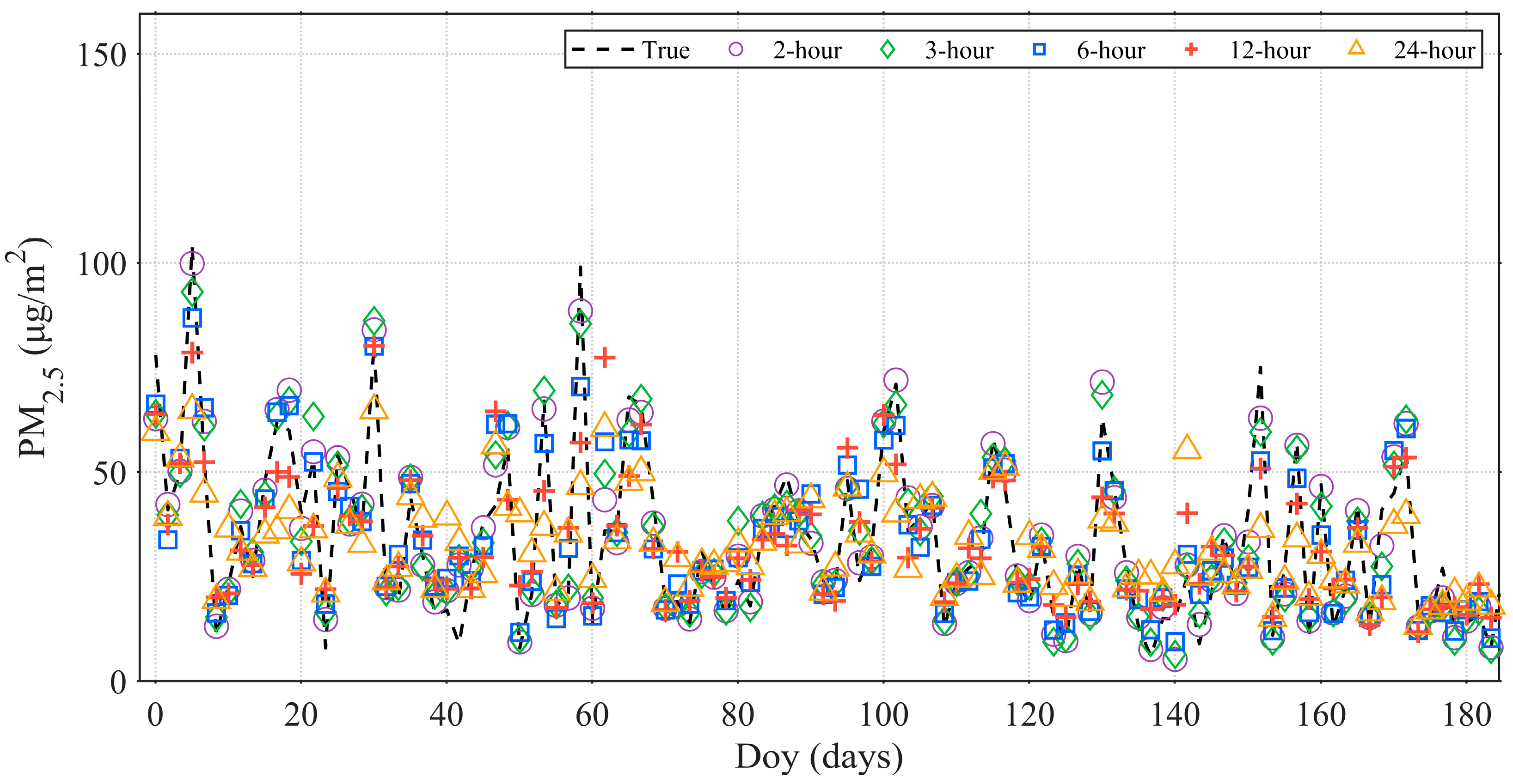
Figure 6 presents the predicted and actual PM_2.5 concentration for 2 h, 3 h, 6 h, 12 h, and 24 h using the RF-LSTM fusion algorithm. Predictions for 2 h, 3 h, and 6 h were very close to the actual PM_2.5 concentration, demonstrating its strong performance in short-term prediction. However, the deviations between predicted and actual PM_2.5 concentration increased significantly for the 12 h and 24 h predictions, indicating that the predicted performance of the RF-LSTM decreases as the forecasting time increases to more than 6 h. However, the results indicate that the RF-LSTM captures the overall trends of PM_2.5 concentration effectively.

Table 6. The accuracy of 2 h, 3 h, 6 h, 12 h, and 24 h PM_2.5 concentration prediction models using the RF-LSTM fusion algorithm $\left(\mathsf{\mu }\mathrm{g}/{\mathrm{m}}^3\right)$.

Time	Bias	RMSE	MAE	MAPE (%)
2 h	0.02	5.63	3.61	13.82
3 h	−0.02	6.87	3.66	18.28
6 h	−0.23	9.86	3.58	28.33
12 h	−0.61	12.64	8.82	38.19
24 h	−1.26	15.33	10.76	48.22

presents the bias, RMSE, MAE, and MAPE of PM_2.5 prediction models using RF-LSTM across a prediction time of 2–24 h. For the 2 h model, the results showed a bias of 0.02 $\mathsf{\mu }\mathrm{g}/{\mathrm{m}}^3$, an RMSE of 5.63 $\mathsf{\mu }\mathrm{g}/{\mathrm{m}}^3$, an MAE of 3.61 $\mathsf{\mu }\mathrm{g}/{\mathrm{m}}^3$, and a MAPE of 13.82%. For the 3 h model, their corresponding values were −0.02 $\mathsf{\mu }\mathrm{g}/{\mathrm{m}}^3$, 6.87 $\mathsf{\mu }\mathrm{g}/{\mathrm{m}}^3$, 3.66 $\mathsf{\mu }\mathrm{g}/{\mathrm{m}}^3$, and 18.28%, respectively. For the 6 h model, the bias, RMSE, MAE, and MAPE were −0.23 $\mathsf{\mu }\mathrm{g}/{\mathrm{m}}^3$, 9.86 $\mathsf{\mu }\mathrm{g}/{\mathrm{m}}^3$, 3.66 $\mathsf{\mu }\mathrm{g}/{\mathrm{m}}^3$, and 28.28%, respectively. These results indicate that the 2–6 h models achieve high stability and accuracy in short-term prediction. However, their accuracy decreases as the forecasting time increases.

The bias, RMSE, MAE, and MAPE of the 12 h PM_2.5 concentration prediction models were −0.61 $\mathsf{\mu }\mathrm{g}/{\mathrm{m}}^3$, 12.64 $\mathsf{\mu }\mathrm{g}/{\mathrm{m}}^3$, 8.82 $\mathsf{\mu }\mathrm{g}/{\mathrm{m}}^3$, and 38.33%, respectively. For the 24 h PM_2.5 concentration prediction model, their corresponding metrics increased to −1.26 $\mathsf{\mu }\mathrm{g}/{\mathrm{m}}^3$, 15.33 $\mathsf{\mu }\mathrm{g}/{\mathrm{m}}^3$, 10.76 $\mathsf{\mu }\mathrm{g}/{\mathrm{m}}^3$, and 48.22%, respectively. An obvious error accumulation was observed, but they remained effective in capturing the overall PM_2.5 prediction trend. This indicates that increased and uncertain complexity affects longer-term prediction accuracy.

5. Conclusions and Discussion

The data of GNSS, meteorological, and environmental monitoring stations in Suzhou city from 2021 to 2023 were used to construct a PM_2.5 concentration prediction model based on a sliding window and RF-LSTM fusion algorithm. The bias, RMSE, MAE, and MAPE of LSTM, MLP, Bi-LSTM, RF-MLP, and RF-LSTM PM_2.5 concentration models were compared to evaluate their prediction accuracy. The main conclusions are as follows.

The selection of sliding windows has a substantial impact on the performance of PM_2.5 prediction models. A comparative analysis of 6 h, 12 h, 24 h, 48 h, and 72 h window lengths was conducted in this study. The RMSEs were 8.68 $\mathsf{\mu }\mathrm{g}/{\mathrm{m}}^3$, 7.30 $\mathsf{\mu }\mathrm{g}/{\mathrm{m}}^3$, 6.88 $\mathsf{\mu }\mathrm{g}/{\mathrm{m}}^3$, 6.90 $\mathsf{\mu }\mathrm{g}/{\mathrm{m}}^3$, and 6.85 $\mathsf{\mu }\mathrm{g}/{\mathrm{m}}^3$, respectively. The RMSEs of 24 h, 48 h, and 72 h were at the same level, indicating stable prediction accuracy after the window length reaches 24 h or more. Consequently, a 24 h sliding window was selected.

The bias, RMSE, MAE, and MAPE of the 1 h RF-LSTM PM_2.5 concentration prediction models were −0.02 $\mathsf{\mu }\mathrm{g}/{\mathrm{m}}^3$, 4.36 $\mathsf{\mu }\mathrm{g}/{\mathrm{m}}^3$, 2.63 $\mathsf{\mu }\mathrm{g}/{\mathrm{m}}^3$, and 9.30%. The RF-LSTM results represented accuracy improvements of 34.7%, 29.3%, 23.2%, and 25.9% over the LSTM, Bi-LSTM, MLP, and RF-MLP algorithms, indicating that the RF-LSTM fusion algorithm is better at predicting short-term PM_2.5 concentration. For the 2, 3, 6, 12, and 24 h RF-LSTM PM_2.5 concentration prediction models, the RMSEs were 5.63 $\mathsf{\mu }\mathrm{g}/{\mathrm{m}}^3$, 6.87 $\mathsf{\mu }\mathrm{g}/{\mathrm{m}}^3$, 9.86 $\mathsf{\mu }\mathrm{g}/{\mathrm{m}}^3$, 12.64 $\mathsf{\mu }\mathrm{g}/{\mathrm{m}}^3$, and 15.33 $\mathsf{\mu }\mathrm{g}/{\mathrm{m}}^3$, respectively. These results indicate that prediction accuracy declines as the prediction time increases, but they remain effective in capturing the overall PM_2.5 prediction trend.

Only one GNSS and one meteorological station were used in the study, the limited spatial data fails to capture the significant geographical and meteorological effects on PM_2.5 concentration in a complex urban environment. The spatial PM_2.5 concentration prediction model for whole Suzhou region should be considered in the next study.

References

1. Tsai, F.C.; Smith, K.R.; Vichit-Vadakan, N.; Ostro, B.D.; Chestnut, L.G.; Kungskulniti, N. Indoor/outdoor PM10 and PM2.5 in Bangkok, Thailand. J. Expo. Sci. Environ. Epidemiol. 2000, 10, 15–26. [Google Scholar] [CrossRef] [PubMed]
2. Zhao, R.; Gu, X.; Xue, B.; Zhang, J.; Ren, W. Short period PM2.5 prediction based on multivariate linear regression model. PLoS ONE 2018, 13, e0201011. [Google Scholar] [CrossRef]
3. Wang, Z.; Chen, P.; Wang, R.; An, Z.; Qiu, L. Estimation of PM2.5 concentrations with high spatiotemporal resolution in Beijing using the ERA5 dataset and machine learning models. Adv. Space Res. 2023, 71, 3150–3165. [Google Scholar] [CrossRef]
4. Wei, P.; Xie, S.; Huang, L.; Zhu, G.; Tang, Y.; Zhang, Y. Prediction of PM2.5 concentration in Guangxi region, China based on MLR-ARIMA. J. Phys. Conf. Ser. 2021, 2006, 23–25. [Google Scholar] [CrossRef]
5. Hu, T.; Wang, X.; Liu, T.; Liu, H. A Novel Deep Learning Model for Subway PM2.5 Prediction Using Neighborhood Component Analysis and Convolutional Latent Variables. IEEE Trans. Instrum. Meas. 2025, 74, 2530309. [Google Scholar] [CrossRef]
6. Li, Q.; Chen, Y.; Karimian, H.; Fan, Q.; Abbasi, R. An Integrated Modeling Framework for PM2.5 Source Apportionment in the Yangtze River Delta Using WRF-CMAQ and ISAM. Atmos. Pollut. Res. 2025, 16, 102637. [Google Scholar] [CrossRef]
7. Mohammadi, F.; Teiri, H.; Hajizadeh, Y.; Abdolahnejad, A.; Ebrahimi, A. Prediction of atmospheric PM2.5 level by machine learning techniques in Isfahan, Iran. Sci. Rep. 2024, 14, 2109. [Google Scholar] [CrossRef]
8. Garcia, A.; Santa-Helena, E.; De Falco, A.; de Paula Ribeiro, J.; Gioda, A.; Gioda, C.R. Toxicological effects of fine particulate matter (PM2.5): Health risks and associated systemic injuries—Systematic review. Water Air Soil Pollut. 2023, 234, 346. [Google Scholar] [CrossRef]
9. Chan, C.K.; Yao, X. Air pollution in mega cities in China. Atmos. Environ. 2008, 42, 1–42. [Google Scholar] [CrossRef]
10. Yang, J.; Yan, R.; Nong, M.; Liao, J.; Li, F.; Sun, W. PM2.5 concentrations forecasting in Beijing through deep learning with different inputs, model structures and forecast time. Atmos. Pollut. Res. 2021, 12, 101168. [Google Scholar] [CrossRef]
11. Zhou, G.; Xu, J.; Xie, Y.; Chang, L.; Gao, W.; Gu, Y.; Zhou, J. Numerical air quality forecasting over eastern China: An operational application of WRF-Chem. Atmos. Environ. 2017, 153, 94–108. [Google Scholar] [CrossRef]
12. Liu, S.-K.; Cai, S.; Chen, Y.; Xiao, B.; Chen, P.; Xiang, X.-D. The effect of pollutional haze on pulmonary function. J. Thorac. Dis. 2016, 8, 41–56. [Google Scholar] [CrossRef]
13. Li, W. Modeling Study of Online Public Concern on PM2.5 Pollution in China Based on Baidu index. Ph.D. Thesis, Dalian University of Technology, Dalian, China, 2023. [Google Scholar] [CrossRef]
14. Lai, X.; Li, H.; Pan, Y. A combined model based on feature selection and support vector machine for PM2.5 prediction. J. Intell. Fuzzy Syst. 2021, 40, 10099–10113. [Google Scholar] [CrossRef]
15. Harish Kumar, K.; Gad, I. Time series analysis for prediction of PM2.5 using seasonal autoregressive integrated moving average (SARIMA) model on Taiwan air quality monitoring network data. J. Comput. Theor. Nanosci. 2020, 17, 3964–3969. [Google Scholar] [CrossRef]
16. Xie, S.; Zhang, Y.; Huang, L.; Wei, P.; Zhang, J.; Tang, Y. Multi-scale PM2.5 concentration prediction Considering PWV in Guangxi. J. Guilin Univ. Technol. 2024, 44, 90–95. [Google Scholar] [CrossRef]
17. Li, R.; Wu, S.; Wang, X.; Sun, K.; Dai, G.; Fan, M.; Ma, L.; Zheng, X.; Long, W.; Meng, F. PM2.5 and PM10 vertical distribution retrieval methods based on coherent Doppler lidar via machine learning: For haze and dust in Qingdao. Atmos. Environ. 2025, 395, 121351. [Google Scholar] [CrossRef]
18. Salman, H.A.; Kalakech, A.; Steiti, A. Random forest algorithm overview. Babylon. J. Mach. Learn. 2024, 2024, 69–79. [Google Scholar] [CrossRef] [PubMed]
19. Ju, Y. Predictive analysis of PM2.5 in Nanjing under Multiple Machine Learning Models. Environ. Sci. Surv. 2025, 44, 46–52. [Google Scholar] [CrossRef]
20. Guo, Q.; Yao, Y.; Zhou, Y. PM2.5 random forest prediction model incorporating GNSS meteorological parameters. Sci. Surv. Mapp. 2021, 46, 37–42+56. [Google Scholar] [CrossRef]
21. Wang, W.; Liang, R.; Qi, Y.; Cui, X.; Liu, J. Prediction model of spontaneous combustion risk of extraction borehole based on PSO-BPNN and its application. Sci. Rep. 2024, 14, 5. [Google Scholar] [CrossRef]
22. Wu, Y.; Zhang, Z.; Qi, X.; Hu, W.; Si, S. Prediction of flood sensitivity based on Logistic Regression, eXtreme Gradient Boosting, and Random Forest modeling methods. Water Sci. Technol. 2024, 89, 2605–2624. [Google Scholar] [CrossRef]
23. Choi, S.W.; Kim, B.H. Applying PCA to deep learning forecasting models for predicting PM2.5. Sustainability 2021, 13, 3726. [Google Scholar] [CrossRef]
24. Chang, Y.-S.; Chiao, H.-T.; Abimannan, S.; Huang, Y.-P.; Tsai, Y.-T.; Lin, K.-M. An LSTM-based aggregated model for air pollution forecasting. Atmos. Pollut. Res. 2020, 11, 1451–1463. [Google Scholar] [CrossRef]
25. Kristiani, E.; Lin, H.; Lin, J.-R.; Chuang, Y.-H.; Huang, C.-Y.; Yang, C.-T. Short-Term Prediction of PM2.5 Using LSTM Deep Learning Methods. Sustainability 2022, 14, 2068. [Google Scholar] [CrossRef]
26. Yang, X.; Xiao, D.; Bai, H.; Tang, J.; Wang, W. Spatiotemporal distributions of PM2.5 concentrations in the Beijing–Tianjin–Hebei region from 2013 to 2020. Front. Environ. Sci. 2022, 10, 842237. [Google Scholar] [CrossRef]
27. Fang, C.; Wang, Z.; Xu, G. Spatial-temporal characteristics of PM2.5 in China: A city-level perspective analysis. J. Geogr. Sci. 2016, 26, 1519–1532. [Google Scholar] [CrossRef]
28. Li, T.; Hua, M.; Wu, X. A hybrid CNN-LSTM model for forecasting particulate matter (PM2.5). IEEE Access 2020, 8, 26933–26940. [Google Scholar] [CrossRef]
29. Su, Y.; Li, J.; Liu, L.; Guo, X.; Huang, L.; Hu, M. Application of CNN-LSTM Algorithm for PM2.5 Concentration Forecasting in the Beijing-Tianjin-Hebei Metropolitan Area. Atmosphere 2023, 14, 1392. [Google Scholar] [CrossRef]
30. Shang, J.; Zhang, P.; Wang, Y.; Liu, Y.; Wang, H.; Li, S. PM2.5 Concentration Prediction in the Beijing–Tianjin–Hebei Region Based on ERA5 Stratified PWV and Atmospheric Pollutants. Atmosphere 2025, 16, 269. [Google Scholar] [CrossRef]
31. Wu, F.; Min, P.; Jin, Y.; Zhang, K.; Liu, H.; Zhao, J.; Li, D. A novel hybrid model for hourly PM2.5 prediction considering air pollution factors, meteorological parameters and GNSS-ZTD. Environ. Model. Softw. 2023, 167, 105780. [Google Scholar] [CrossRef]
32. Zhou, X.; Xie, M.; Zhao, M.; Wang, Y.; Luo, J.; Lu, S.; Li, J.; Liu, Q. Pollution characteristics and human health risks of PM2.5-bound heavy metals: A 3-year observation in Suzhou, China. Environ. Geochem. Health 2023, 45, 5145–5162. [Google Scholar] [CrossRef]
33. Li, L.; Li, Y.; He, Q.; Wang, X. Weighted Mean Temperature Modelling Using Regional Radiosonde Observations for the Yangtze River Delta Region in China. Remote Sens. 2022, 14, 1909. [Google Scholar] [CrossRef]
34. Wang, Z.; Chai, H.; Ming, L.; Ye, Y.; Ma, H.; Chen, P. Estimation of PM2.5 concentration in southern China using stacked machine learning models based on GNSS and radiosonde precipitable water vapor. Adv. Space Res. 2025, 76, 1338–1354. [Google Scholar] [CrossRef]
35. Li, K.; Li, L.; Tang, J.; Dick, G.; Wickert, J.; Yu, H.; He, Q.; Dong, Z. Research on the PWV prediction model based on the ERA5-PWV calibration and WOA-RNN-BiLSTM-multihead-attention fusion algorithms. Atmos. Res. 2025, 325, 108238. [Google Scholar] [CrossRef]
36. Li, K.; Li, L.; Hu, A.; Pan, J.; Ma, Y.; Zhang, M. Research on modeling weighted average temperature based on the machine learning algorithms. Atmosphere 2023, 14, 1251. [Google Scholar] [CrossRef]
37. Liu, Y.; Wang, Y.; Zhang, J. New machine learning algorithm: Random forest. In Proceedings of the International Conference on Information Computing and Applications, Chengde, China, 14–16 September 2012; Volume 7473, pp. 246–252. [Google Scholar] [CrossRef]
38. Raileanu, L.E.; Stoffel, K. Theoretical comparison between the gini index and information gain criteria. Ann. Math. Artif. Intell. 2004, 41, 77–93. [Google Scholar] [CrossRef]
39. Hochreiter, S.; Schmidhuber, J. Long short-term memory. Neural Comput. 1997, 9, 1735–1780. [Google Scholar] [CrossRef] [PubMed]
40. Mohammadi, M.; Jamshidi, S.; Rezvanian, A.; Gheisari, M.; Kumar, A. Advanced fusion of MTM-LSTM and MLP models for time series forecasting: An application for forecasting the solar radiation. Meas. Sens. 2024, 33, 101179. [Google Scholar] [CrossRef]
41. Drobnič, F.; Kos, A.; Pustišek, M. On the interpretability of machine learning models and experimental feature selection in case of multicollinear data. Electronics 2020, 9, 761. [Google Scholar] [CrossRef]
42. Lakshmi, S.; Krishnamoorthy, A. Effective Multi-Step PM2.5 and PM10 Air Quality Forecasting Using Bidirectional ConvLSTM Encoder-Decoder with STA Mechanism. IEEE Access 2024, 12, 179628–179647. [Google Scholar] [CrossRef]
Figure 1. Locations of GNSS, meteorological, and environmental stations in Suzhou city.
Atmosphere 16 01147 g001
Figure 2. The structure diagram of LSTM cell units.
Atmosphere 16 01147 g002
Figure 3. The schematic diagram of the sliding window.
Atmosphere 16 01147 g003
Figure 4. Flowchart of PM2.5 concentration prediction model using RF-LSTM.
Atmosphere 16 01147 g004
Figure 5. Comparison of 1 h predicted PM2.5 concentration (a) and truth using RF-LSTM fusion algorithms and their fitting plot (b).
Atmosphere 16 01147 g005
Figure 6. Comparison of actual PM2.5 concentration with RF-LSTM predicted at 2 h, 3 h, 6 h, 12 h, and 24 h.
Atmosphere 16 01147 g006