Article

Sources and Trends of CO, O3, and Aerosols at the Mount Bachelor Observatory (2004–2022)

by
Noah Bernays
1,
Jakob Johnson
1 and
Daniel Jaffe
1,2,*
1
School of Science, Technology, Engineering and Mathematics, University of Washington Bothell, 18115 Campus Way NE, Bothell, WA 98011, USA
2
Department of Atmospheric Sciences, University of Washington, 3920 Okanogan Lane, Seattle, WA 98195, USA
*
Author to whom correspondence should be addressed.
Atmosphere 2025, 16(1), 85; https://doi.org/10.3390/atmos16010085
Submission received: 3 December 2024 / Revised: 12 January 2025 / Accepted: 13 January 2025 / Published: 15 January 2025
(This article belongs to the Special Issue Measurement and Variability of Atmospheric Ozone)

Abstract

:
Understanding baseline O3 is important as it defines the fraction of O3 coming from global sources and not subject to local control. We report the occurrence and sources of high baseline ozone days, defined as a day where the daily maximum 8 h average (MDA8) exceeds 70 ppb, as observed at the Mount Bachelor Observatory (MBO, 2.8 km asl) in Central Oregon from 2004 to 2022. We used various indicators and enhancement ratios to categorize each high-O3 day: carbon monoxide (CO), aerosol scattering, the water vapor mixing ratio (WV), the aerosol scattering-to-CO ratio, backward trajectories, and the NOAA Hazard Mapping System Fire and Smoke maps. Using these, we identified four causes of high-O3 days at the MBO: Upper Troposphere/Lower Stratosphere intrusions (UTLS), Asian long-range transport (ALRT), a mixed UTLS/ALRT category, and events enhanced by wildfire emissions. Wildfire sources were further divided into two categories: smoke transported in the boundary layer to the MBO and smoke transported in the free troposphere from more distant fires. Over the 19-year period, 167 high-ozone days were identified, with an increasing fraction due to contributions from wildfire emissions and a decreasing fraction of ALRT events. We further evaluated trends in the O3 and CO data distributions by season. For O3, we found an overall increase in the mean and median values of 2.2 and 1.5 ppb, respectively, from the earliest part of the record (2004–2013) compared to the later part (2014–2022), but no significant linear trends in any season. For CO, we found a significant positive trend in the summer 95th percentiles, associated with increasing fires in the Western U.S., and a strong negative trend in the springtime values at all percentiles (1.6% yr−1 for 50th percentile). This decline was likely associated with decreasing emissions from East Asia. Overall, our findings are consistent with the positive trend in wildfires in the Western United States and the efforts in Asia to decrease emissions. This work demonstrates the changing influence of these two source categories on global background O3 and CO.

1. Introduction

Carbon monoxide (CO), ozone (O3), and aerosols are key components of the global atmosphere. Ozone is an important pollutant, greenhouse gas, and source of hydroxyl radical (OH) in the troposphere. O3 is a secondary pollutant, formed in the troposphere by the photochemical reaction of NOx (NO + NO2) and Volatile Organic Compounds (VOCs) [1,2]. Ozone is toxic to humans, and concentrations in many urban areas exceed health standards due to photochemical production [3,4]. In the U.S., the National Ambient Air Quality Standard (NAAQS) for O3 is an annual fourth-highest, maximum daily 8 h average (MDA8) of 70 parts per billion by volume (ppb) or less, averaged over a three-year period [5]. The terms “background” and “baseline” O3 have been used in several different contexts in relation to non-locally produced O3. In the Tropospheric Ozone Assessment Report, a station was defined as a “background” station if it was minimally influenced by local processes [6,7]. In Hemispheric Transport of Air Pollution, baseline O3 was defined as “the distribution of O3 observations at a rural or remote site that has not been influenced by recent, local emissions” [8]. For our analysis, we use this definition and treat the terms “background” and “baseline” as synonymous. As background O3 is a significant fraction of the U.S. NAAQS (40–70%), it is essential to understand the occurrence and causes of high-ozone events [9]. O3 is also produced naturally in the stratosphere and can contribute to the tropospheric O3 budget via stratosphere–troposphere air exchange. Because of its significant impact on the global atmosphere, it is important to document long-term trends in O3 [10,11].
CO and aerosols are emitted directly from human activities and biomass burning. The reaction of CO with the hydroxyl radical (OH) is the dominant loss process for OH and is thus a key constituent in the global atmosphere [12]. Aerosols are important climate-forcing agents, causing both positive and negative climate forcing, depending on their altitude and relative amounts of light scattering vs. absorption [13]. In addition to their importance in atmospheric processes, CO and aerosols are excellent tracers of source type and have lifetimes that are sufficiently long to demonstrate inter-continental transport [14,15].
In the Pacific Northwest, previous studies of background O3 have identified three primary sources: natural intrusions from the Upper Troposphere/Lower Stratosphere (UTLS), Asian long-range transport of pollution (ALRT), and ozone produced from regional wildfire smoke (RWS). In this study, we split RWS events into two categories: FT-Smoke and BL-Smoke (wildfire smoke transported in the free troposphere and boundary layer, respectively). UTLS events are common in the Eastern Pacific, as a semi-permanent anticyclone creates a baroclinic zone ideal for the descent of stratospheric airmasses [16,17]. ALRT events are most common in spring and have generally become less common after 2015; their compositions vary, but those containing a high ozone concentration contain significant anthropogenic pollution from East Asia and China and may also include some contribution from Siberian wildfires [18,19]. RWS events are common in late summer and autumn and are mostly associated with smoke from fires in the Pacific Northwest, although fires in other parts of Western North America may also contribute [15,19]. Wildfire emissions produce VOCs and nitrogen species, such as NOx and peroxyacetyl nitrate (PAN). PAN is particularly important as it has a long lifetime in the free troposphere and can be thermally decomposed back to NOx, causing ozone concentrations in smoke plumes to vary based on plume age [20].
Until the mid-2010s, O3 produced from Asian emission sources was increasing and contributing to rising North American background ozone levels [18,21,22]. However, beginning in the 2000s, East Asian countries such as Japan and Korea began lowering ozone precursors like NOx and particulate matter (PM) [23,24,25]. Additionally, in 2013, China, Asia’s largest polluter, implemented their Clean Air Action plan, emphasizing “ultra-low” emissions standards from power facilities, resulting in lower NOx and PM2.5 emissions [26,27,28]. Using the GEOS-Chem global chemical transport model, Miyazaki et al. (2020) suggest that the reduction in Chinese NOx emissions should reduce the occurrence of Asian O3 over Western North America [29].
While anthropogenic emissions play a key role in background O3, biomass burning is also a significant factor. Recent aircraft studies suggest that biomass burning is an important source of O3 throughout the free troposphere (FT) [30]. Ziemke et al. (2009) estimate that wildfires add 4–5% to the tropospheric ozone burden [31]. In the United States and Canada, climate change has heightened the frequency and intensity of the wildfire season [32,33]. In the Western U.S., a significant positive trend in burned area equivalent to 20 additional large fires is estimated every decade from 1973 to 2012 [34]. As smoke events intensify, wildfires will continue to possess unprecedented sway over seasonal air quality [35,36,37].
The Mt. Bachelor Observatory (MBO) is a mountain-top atmospheric chemistry observatory situated in central Oregon (43.9775° N, 121.6861° W; 2.8 km above sea level). Ozone, carbon monoxide, 3λ aerosol scattering coefficients, and meteorology have been observed nearly continuously since 2004, with other species (NOx, NOy, Hg, VOCs, etc.) measured as needed for specific research campaigns. Being on the summit of an isolated stratovolcano, the MBO exhibits a strong diurnal airflow pattern, with boundary-layer-influenced (BLI) air being pulled upslope during the day, and FT air brought to the summit observatory at night [14]. FT events can be distinguished from BLI events based on time of day and water vapor mixing ratio (WV) [15]. Due to the station’s location on the west coast of North America, high altitude, and distance from urban centers, local (U.S.) industrial pollution is rarely observed at the MBO, while high-O3 events from the FT are much more common [15].
The MBO is a unique facility that allows for regular sampling of free tropospheric air to understand the sources of pollutants in the global atmosphere and how these may be changing. Previous studies at the MBO analyzed background ozone trends and examined high-ozone events, sourcing them using enhancements in CO, submicron aerosol scattering, and WV [15,18,19]. Identifications were corroborated using data from various meteorological models, such as the Hybrid Single-Particle Lagrangian Integrated Trajectory (HYSPLIT) model. This paper follows a similar procedure as Ambrose et al. (2011) and Zhang and Jaffe (2017) to identify sources of high-O3 days at the MBO [15,19].
In this work, our goals are to examine how changes in global anthropogenic emissions, natural variations, and/or wildfires may have impacted background O3 at the MBO over the 19-year period between 2004 and 2022. We achieve this by examining tracer ratios and air mass transport on the highest O3 days over this 19-year period. Our results demonstrate significant changes in sources of pollutants to the global atmosphere.

2. Measurements and Other Sources of Data

The MBO is located at the summit of a dormant volcano in Oregon. The mountain is the location of the Mt. Bachelor ski area, and our instrumentation is housed in the top ski lift building located near the summit (2.8 km asl). From 2004 to 2014, O3 was measured with a Dasibi 1008-RS UV photometric analyzer (Glendale, CA, USA) with a total instrument uncertainty of ±2% for O3 > 5 ppb. The Dasibi was zeroed monthly using activated charcoal [14,15]. Since 2014, ozone has been measured with an Acoem Ecotech Serinus 10 UV analyzer (Richmond, VA, USA) with a total instrument uncertainty of ±2% at 30 ppb. The method detection limits (MDL) of the Dasibi and Ecotech O3 analyzers are 1 and 0.5 ppb, respectively. During that time, O3 calibrations were consistently performed using a Dasibi model 1008-RS calibrator (Glendale, CA, USA) or 2B model 306 calibrator (Broomfield, CO, USA) with a total instrument uncertainty of the greater of 3 ppb or 3% of the ozone concentration. Each calibrator was cross-referenced annually to either a primary photometer owned by the state of Washington Department of Ecology or recalibrated by the manufacturer.
CO was measured with a Thermo Electron Corporation (TECO) 48C non-dispersive analyzer (Waltham, MA, USA) for Spring 2004, then with a TECO 48CTL trace level analyzer (Waltham, MA, USA) until April 2012. Both CO instruments had a “total uncertainty <±10% at typical ambient levels” [15]. Since May 2012, CO has been measured with a Picarro G2302 cavity ring-down spectrometer (Santa Clara, CA, USA). The spectrometer is calibrated every 8 h using NOAA calibration standards and has a total instrument uncertainty of ±4% at 100 ppb [38]. Both CO and O3 are reported as mixing ratios or mole fractions in ppb.
Sub-micron total aerosol scattering coefficients (forward and back-scattering) at 3λ (450, 550, 700 nm) were measured using a TSI Inc. model 3563 integrating nephelometer (Shoreview, MN, USA) between 2011 and 2022. Prior to 2011, a Radiance Research M903 nephelometer (Seattle, WA, USA) was used. The total scattering coefficients were corrected for drift and scattering truncation using the Anderson and Ogren (1998) correction [39]. For this analysis, we used only total scattering in the green (550 nm, TSG) reported at ambient pressure and temperature. Total uncertainty for scattering measurements was ±15–20% during biomass burning events, but the precision was estimated at 10%, which was more relevant for comparing values between events [38].
The water vapor mixing ratio was calculated using ambient temperature and relative humidity (RH) values from a Campbell Scientific HMP 45C sensor (Logan, UT, USA), and ambient pressure values from a Vaisala PTB101B pressure transmitter (Louisville, CO, USA). The temperature, RH, and pressure measurement uncertainties were estimated to be <±0.4 °C, <±5% RH, and ±4 mbar [15]. Two temperature/RH sensors were employed, one in a sheltered location at the east side of the summit building, and one in a more exposed (ambient) location on the south side of the building. However, the exposed (ambient) sensor would occasionally ice up and read 100% humidity, even when the actual humidity was less than this value. Water vapor values in this study used the sheltered values, when available, and the ambient values when sheltered values were not available.
Backward air mass trajectories (between 24 and 240 h back in time, depending on the nature of the plume) were calculated at the start hour of the event’s O3 MDA8 using NOAA’s HYSPLIT model version 4 [40]. These were calculated at arrival heights of 1000, 1500, and 2000 m above ground level to account for the summit height relative to the model ground elevation. Since the model ground elevation was estimated to be 1300 m above mean sea level (amsl), the three input heights represented 2300, 2800, and 3300 m amsl, respectively, bracketing the summit height of 2763 m amsl. GDAS (1 degree, global, 2006–present) meteorology files were used in the model, and the location of MBO was input at the following coordinates: 43.9775° N, 121.6861° W.
NOAA Hazard Mapping System (HMS) Fire and Smoke map products were downloaded for each smoke event. By inputting the smoke and fire points’ KML files into Google Earth, large fires could be placed along the HYSPLIT back-trajectories to determine the source of the high-O3 event. Archived HMS files can be located here: https://satepsanone.nesdis.noaa.gov/pub/FIRE/web/HMS/ (accessed on 12 January 2025).

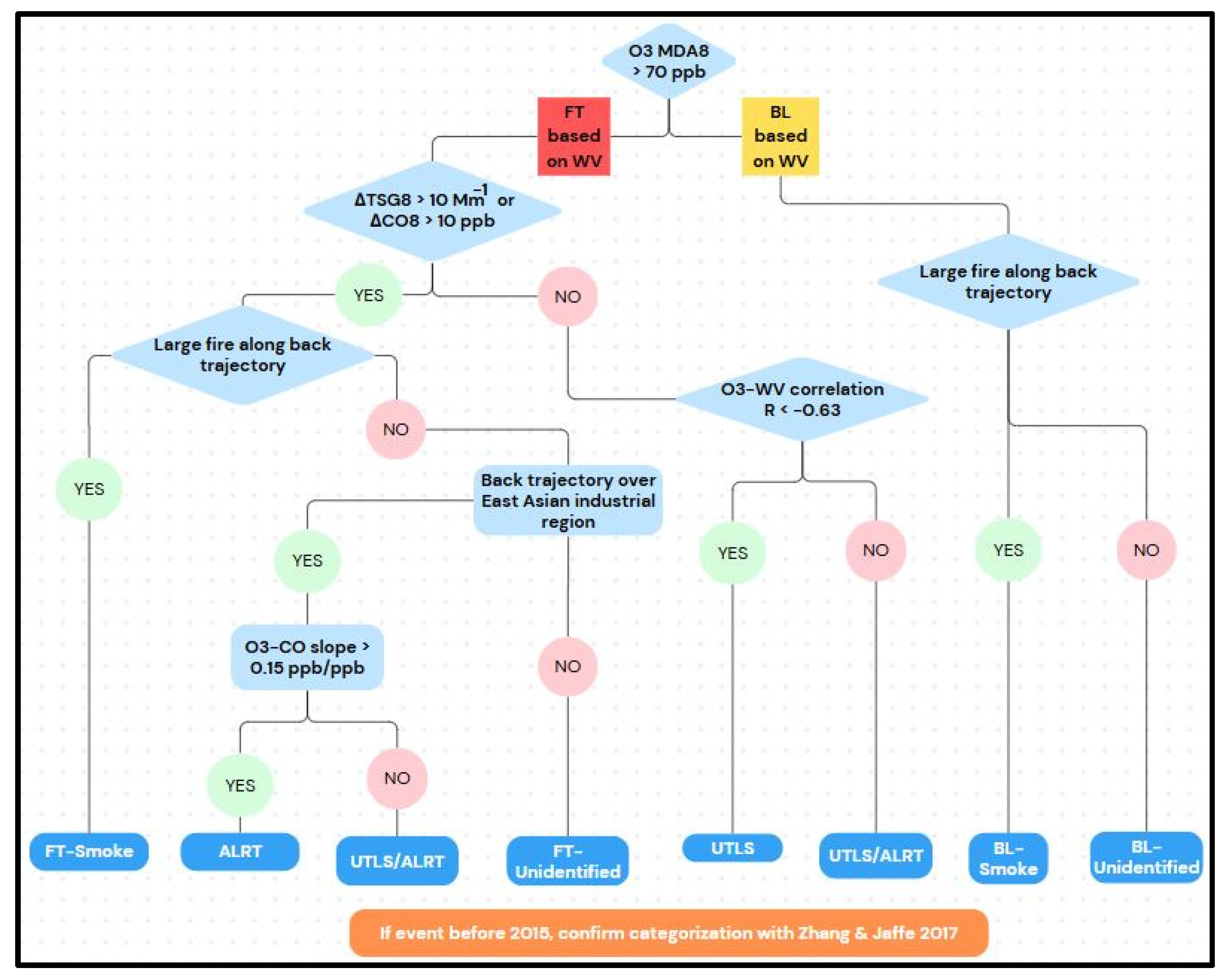
3. Plume Identification and Trend Analysis Methodology
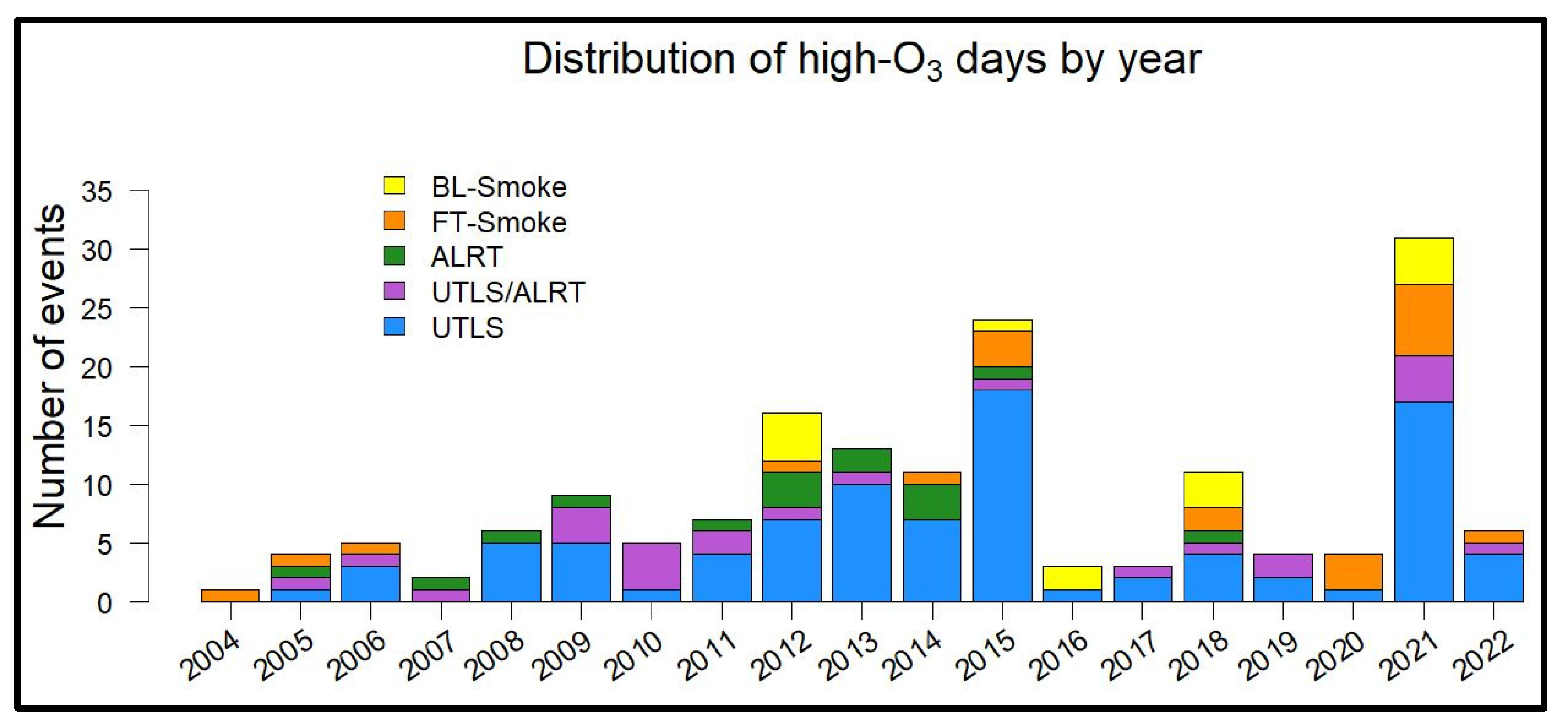
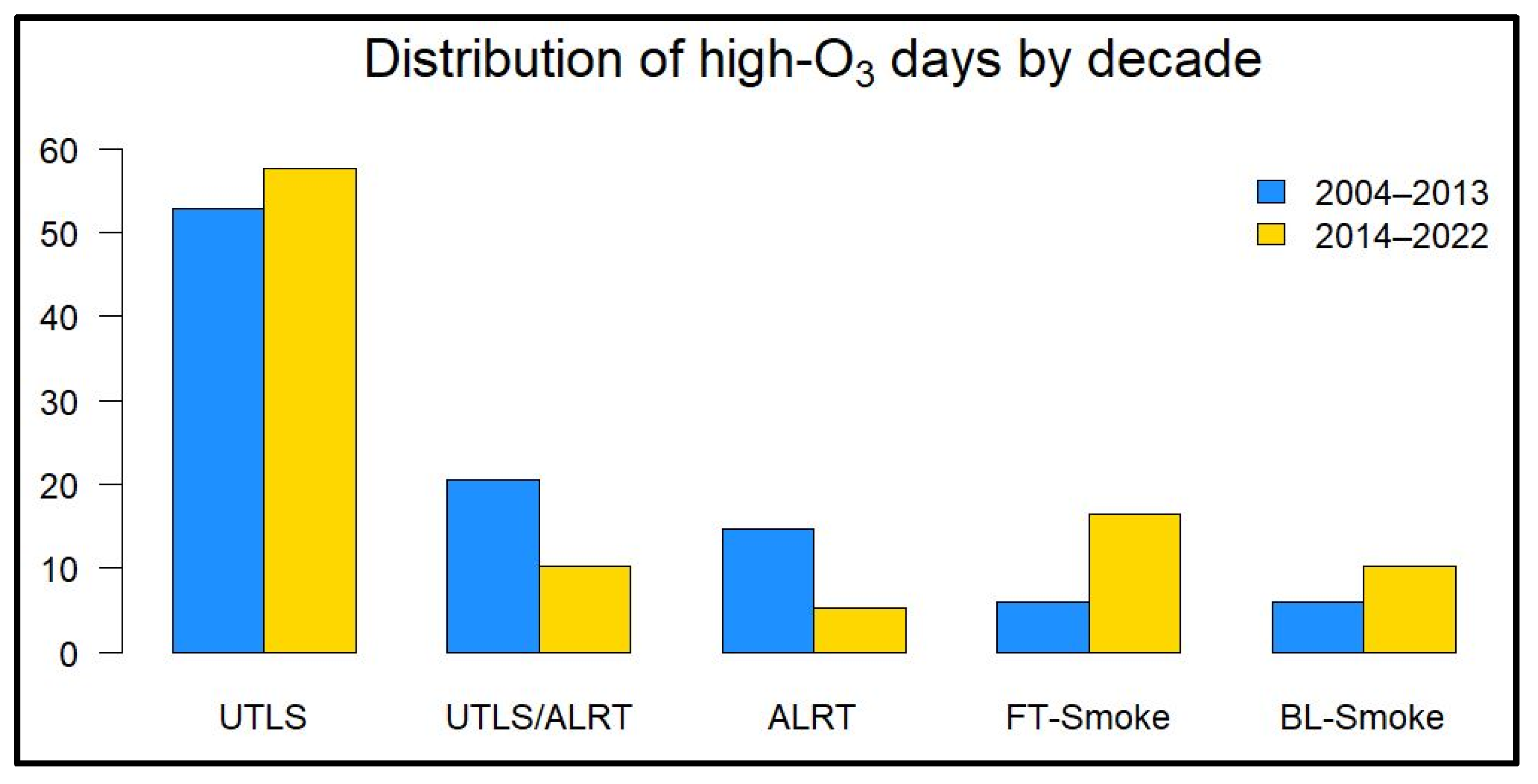
For plume identification, we used hourly data from 2004 to 2022, and “events” were defined as any 8 h period with an O3 MDA8 greater than 70.0 ppb. To prevent double-counting data in sequential days of high O3, any single hour could only be in one 8 h period. The day with the lower of the two O3 MDA8’s was removed (the 8 h periods starting at the indicated times were removed from the final event list: 3 July 2015 23:00, 13 September 2020 0:00, 8 February 2021 23:00, 12 July 2021 23:00, 15 August 2021 23:00, 5 September 2021 0:00 GMT). If an event did not include 6 or more hourly averages of O3, we removed it from the list of events (4 August 2009, 5 January 2016, 26 October 2016). For each 8 h period that exceeded 70.0 ppb, the concurrent CO, WV, and ambient TSG hourly data were averaged to form corresponding 8 h tracer averages. These values were called CO8, WV8, and TSG8, respectively. Previously, we determined free tropospheric water vapor distributions for that location from nearby radiosonde data [15,19]. These values were used to compute monthly free troposphere/boundary layer (FT/BL) cutoff values, as shown in Table 1 below. An airmass was from the free troposphere if WV8 in that airmass was lower than the corresponding monthly cutoff value. Plumes with WV8 values greater than the cutoff were considered BL-influenced (BLI).
For each 8 h value, we calculated the enhancement over the background value (ΔO38, ΔCO8, ΔTSG8, and ΔWV8). Background values for each species were determined using the median of 30 days of hourly averages, 15 days on either side of the event start hour. Background TSG values for particularly smoky periods (August 2015, August 2018, and 20 August–7 September 2021) used the median of 60 days of hourly averages, 30 days on either side of the event start hour.
To examine tracer relationships, we calculated slopes and Pearson correlation coefficients between TSG and CO, O3 and CO, and O3 and WV. We used RMA regression (slope = σY/σX) of the hourly data for each 8 h event, plus 4 h on either side of the event. For example, the slope of the TSG-CO relationship used 16 hourly values for each tracer (8 h of the event + 4 before + 4 after).
We classified each event based on the major source category (Upper Troposphere/Lower Stratosphere or “UTLS”, Asian long-range transport or “ALRT”, a mixed category “UTLS/ALRT”, free troposphere smoke or “FT-Smoke”, boundary layer smoke or “BL-Smoke”, and “FT-Unidentified” or “BL-Unidentified” if the plume had no clear source). If the event was BL-influenced (determined by WV cutoffs as described above), had a significant HMS smoke plume, and the HYSPLIT back trajectory passed through a known fire source, the event was labeled “BL-Smoke”. If no fire could be identified, the event was classified as “BL-Unidentified”, although no events fell into this category.
If the event was from the free troposphere, the plume’s pollutant tracers were inspected. If CO8 increased by more than 10 ppb over its background value, or TSG8 increased by more than 10 Mm−1 over its background, it was considered “enhanced”. If the plume was enhanced, and the HYSPLIT back-trajectory passed near a significant wildfire, the event was labeled “FT-Smoke”. If there was no large fire but the trajectory passed over an East Asian industrial region, the plume’s O3–CO slope was inspected. The plume was classified as “ALRT” if the slope was greater than 0.15 ppb/ppb and as a mixed “UTLS/ALRT” category if not. This mixed category of events, used by Zhang and Jaffe (2017), exhibited characteristics of both UTLS and ALRT plumes, which likely have O3 from both sources [19].
If the event was in the FT and enhanced categories, but back-trajectories did not show it passing over either a large wildfire or an Asian industrial region, it was classified as “FT-Unidentified” (two events fell into this category). If the event was from the FT, but CO8 or TSG8 were not significantly enhanced, the relationship between O3 and WV was used to classify it. If the correlation R for hourly O3 and WV was less than −0.63 (corresponding to an R2 value of 0.4), then the event was classified as “UTLS”. If the correlation criterion was not met, the event was labeled “UTLS/ALRT”.
After applying this methodology to every event, the assignments were compared to those made by Zhang and Jaffe (2017) [19]. Zhang and Jaffe identified 61 corresponding events. We changed 12 of our events to match theirs (1 from ALRT to FT-Smoke, 3 from UTLS/ALRT to FT-Smoke, and 8 from UTLS to UTLS/ALRT because they had identified specific ALRT sources in those 8 cases). Fourteen of our events remained different from their categorizations (ten of our UTLS events were marked as UTLS/ALRT by Zhang and Jaffe, two of our UTLS/ALRT events were marked as ALRT by them, and two of our ALRT events were marked as UTLS/ALRT by them). Figure 1 below summarizes the procedure for how each event was classified.
Trends in CO and O3 were computed on the hourly data from 2004 to 2022. We report linear quantile regression trends at the 5th, 25th, 50th, 75th, and 95th quantiles by season (Winter = Jan/Feb/Mar, Spring = Apr/May/Jun, Summer = Jul/Aug/Sept, and Fall = Oct/Nov/Dec). We also conducted Mann–Kendall trends tests on the quantile data by season.

4. Results

Figure 2 below provides examples of (a) ALRT, (b) UTLS, (c) BL-Smoke, and (d) FT-Smoke events, with O3 MDA8 start hours of 08, 01, 00, and 08 GMT, respectively. ALRT plumes tended to have more gradual enhancements in CO and TSG (a), as opposed to BL-Smoke and FT-Smoke, which had much higher concentrations of tracers that decreased very quickly (c and d). The chemical identity of a UTLS event (b) was most obvious as all tracers (especially water vapor) decreased, while O3 was enhanced.
Figure 3, below, shows how the FT-Smoke example in Figure 2d was confirmed using HYSPLIT back-trajectories and HMS Fire and Smoke maps.
Each of the three trajectories in the HYSPLIT plot in Figure 3b shows that the plume on 20 August 2021 came over the Pacific Ocean from the west, then veered south–southeast at the western edge of British Columbia 72 h before arriving at MBO. The trajectory goes over the Schneider Springs Fire approximately 30 miles northwest of Yakima, Washington, but may also contain tracers from several fires burning in British Columbia at the time. Small amounts of smoke from the Bull Complex Fires located approximately 60 miles north-northwest of MBO, and directly east of Salem, Oregon, may also have been mixed in. Both the Schneider Springs Fire and Bull Complex Fires are shown in Figure 3a. The origin of the BL-Smoke event on 16 August 2021, in Figure 2c, was likely the Dixie Fire in Redding, CA, with smoke contributions from multiple fire clusters approximately 100 miles southwest of Bend, Oregon (Devil’s Knob Complex, Rough Patch Complex, and Jack Fire).
The slopes and correlations of TSG–CO, O3–CO, and O3–WV were calculated for each event using 16 hourly values as described above. For the regional smoke events (FT-Smoke + BL-Smoke), scattering and TSG were generally well correlated in 21 events (R > 0.7), and the mean TSG–CO slope was 0.59 and 0.63 Mm−1/ppb for the BL-Smoke and FT-Smoke events, respectively. As ALRT plumes travel long distances across the Pacific Ocean, smoke particles can be incorporated into cloud droplets and removed by rainout or impaction. This decreases the concentration of TSG in the plume while CO remains relatively constant. We saw this phenomenon in the ALRT events—out of 15 total ALRT events, 5 were well correlated, 8 were poorly correlated, and 2 had missing TSG–CO data. Of the well-correlated ALRT events, the median TSG–CO slope was 0.19 Mm−1/ppb, significantly lower than the smoke plumes traveling shorter distances.
Using the categorization scheme in Figure 1, 167 events with MDA8 > 70.0 ppb between 2004 and 2022 were identified. Figure 4 and Figure 5 below show the distribution of the event types over the 19-year period. The years 2021, 2015, and 2012 had the largest number of events, with 31, 24, and 17, respectively. Five of the sixteen high-ozone days in 2012 were from regional wildfire smoke due to a heightened fire season. The year 2015 had an unusual cluster of 12 out of its 18 UTLS events occurring in May and June. The year 2021 had 31 high-ozone days, more than any other year. July 2021 exhibited a cluster of eight UTLS events, which led into an active fire season producing nine RWS events with high O3 across July, August, and September.
Figure 5 below summarizes the relative distribution of high-ozone days from 2004–2013 (blue) to 2014–2022 (yellow). The proportion of RWS-related ozone days more than doubled (11% to 27%) between the first decade and the second, the proportion of UTLS events increased from 50% to 58%, and the proportion of ALRT-related (ALRT and UTLS/ALRT) ozone days decreased from 35% to 15%. The data also showed an increase in the average number of high-ozone days at MBO per year, from 7 to 11. Including the 2 FT-Unidentified events in 2012 and 2013, there were a total of 70 and 97 high-O3 events in 2004–2013 and 2014–2022, respectively.
The anomalous UTLS events in 2015 (Figure 4) appeared to be linked to the persistent high-pressure ridge in early summer, but the exact cause of these high-ozone days was unclear. Zhang and Jaffe (2017) reported on this event, finding increased levels of ozone in urban areas caused by enhanced surface temperatures, wind stagnation, and low cloud cover, increasing the monthly average MDA8 at surface monitoring stations across Oregon and Washington [19]. The high pressure and stagnation likely enhanced urban ozone formation, but the data for these days at MBO all exhibited low WV, CO, and TSG, with back-trajectories consistent with UTLS.
A similar phenomenon occurred in 2021, with a cluster of UTLS events following the unprecedented heatwave from 25 June to 2 July [41,42,43]. Following the high-pressure ridge, we observed an unusual number of successive UTLS events similar to the June 2015 heatwave. However, the July 2021 episode did not produce the same heightened ozone concentrations in the lowlands. The 2021 heatwave was temporally much shorter than the 2015 high-pressure event, with strong easterly winds, failing to recreate the prolonged stagnant conditions of 2015.
The 2021 heatwave also intensified drought conditions, drying woodland vegetation and encouraging an unusually early fire season, burning 3354 km2 in Oregon state that year [38,44]. For comparison, from 2002 to 2019, the burned area in Oregon state averaged 2233 km2 per year. Our results identified regional wildfire events interspersed with UTLS events at the end of the episode in mid-July. The increase in RWS days observed in Figure 5 followed the national trend of increasing burn area. From 2001 to 2010, the total burn area in the United States averaged 26,443 km2 per year, which rose to 30,419 km2 per year for 2011–2020 [44].

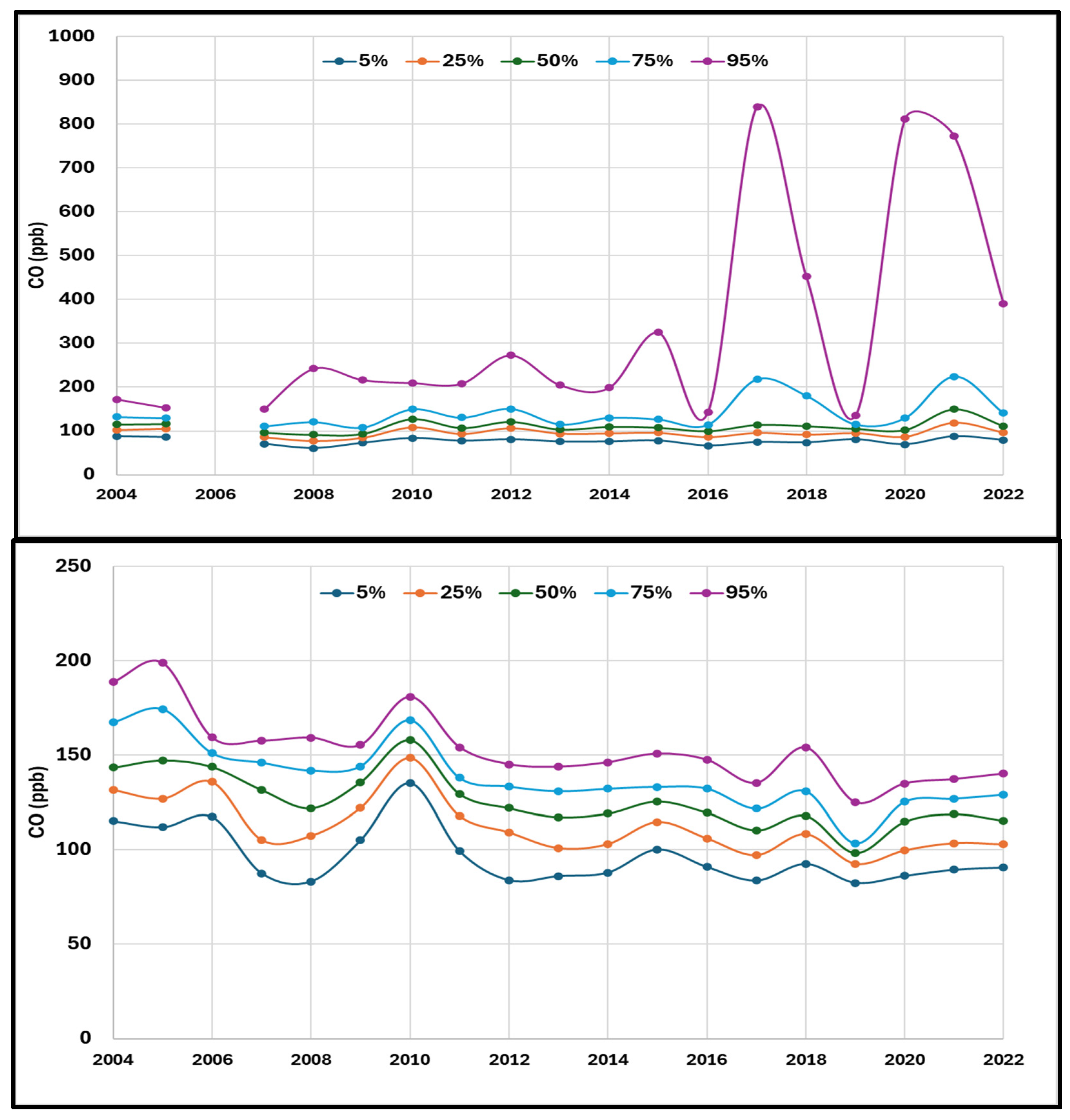
5. Trends in O3 and CO

Table 2 and Table 3 show the percentiles by season and year for both O3 and CO. Figure 6 shows the trends in O3 for spring and summer. We focused on these seasons as these were shown in the past to have the strongest intercontinental transport of pollution and biomass burning, respectively. With an increase in the number of high-O3 days (due to smoke events and increasing UTLS), we might expect to see a significant trend in O3 concentrations at MBO. Indeed, both the mean and median O3 concentrations were significantly higher (p < 0.05) by 2.1 and 1.2 ppb, respectively, in the later decade of the data record (2013–2022) compared to the first 9 years of the data record (2004–2012). However, for O3, we saw no evidence of a significant (p < 0.05) linear trend in any season using either standard quantile regression or the Mann–Kendall tests. At the 95th percentile, O3 showed an increase in summer; however, this was only significant with a p-value of 0.08. Chang et al. (2023) examined trends in the hourly O3 nighttime data from MBO using quantile regression. They reported a small positive trend in the median values (2.7 ppb/decade) using data from 2004 to 2019, but that trend was reduced due to temporary reductions in O3 on a global scale caused by the pandemic. At the MBO, the strong dip in O3 in the spring of 2020 was likely associated with the global pandemic [10]. This was followed by an especially high biomass burning season in the Western U.S. which likely erased any reductions due to global declines in the summer of 2020. O3 in the summer of 2021 was especially high, as was CO in the summers of 2017, 2020, and 2021. These high concentrations were consistent with substantial biomass burning influence in those years.
Figure 7 shows the trends in CO for spring and summer. For CO, we saw a significant positive trend in the 95th percentile in summer, but the most robust trends in CO were decreasing concentrations at all quantiles in spring. This reflected a strong and continuing decline in global emissions of CO [18,45]. From our data, the trend in median CO for spring was −2.0 ppb/year or −1.6% yr−1. These changes are larger than the global mean changes reported by Zheng et al. (2019) but are comparable to the 2% yr−1 decline in East Asian emissions reported by Zheng et al. (2018) for 2005–2016 [45,46].

6. Discussion and Conclusions

Observations of O3, CO, and aerosols at mountaintop background stations are relatively sparse. The Mt. Bachelor Observatory in central Oregon, at 2.8 km amsl, is positioned to sample both free tropospheric and boundary layer-influenced air as airmasses of various source locations arrive at the station depending on local meteorology. This makes the 19-year record of observations particularly valuable. In the early part of the MBO data record (2004–2013), we reported a significant increase in springtime O3, which was attributed to the rapid build-up of emissions from East Asian industrial sources. After that period, we saw no statistically significant trends in O3, but we did see a decline in the frequency of high-O3 events associated with East Asian industrial sources. At the same time, we saw an increase in the frequency of high-O3 days associated with biomass burning sources. Thus, it appears that O3 is decreasingly influenced by Asian emissions and increasingly influenced by biomass burning sources.
For CO, we saw a significant increase at the highest quantile in summer, which was clearly associated with the increase in biomass burning sources in North America. At the same time, we saw a downward trend in CO concentrations in spring for all quantiles, associated with decreasing Asian emissions. The trend in CO was consistent with other observations in the literature and may represent a hemispheric phenomenon or at least a Pacific-wide change in the distribution of this important pollutant.
In summary, our 19-year record of baseline O3 and CO data at the MBO from 2004 to 2022 showed a transition in sources of O3 along the west coast of North America. High-O3 occurrences due to long-range transport of Asian pollution declined, but in its place were an increasing number of high-O3 days due to emissions from regional wildfires. Our results aligned with the timeline of East Asian emissions control, identifying only one ALRT event after 2015 and strongly declining CO concentrations. The data showed a marked increase in the number of regional wildfire-related high ozone days after 2013, consistent with the recent increase in the area burned across North America.

Author Contributions

Conceptualization, D.J. and J.J.; methodology, D.J.; formal analysis, N.B. and J.J.; investigation, J.J.; resources, D.J.; data curation, D.J. and N.B.; writing—original draft preparation, N.B. and J.J.; writing—review and editing, D.J.; visualization, N.B.; supervision, D.J.; funding acquisition, D.J. All authors have read and agreed to the published version of the manuscript.

Funding

This research was funded by the National Science Foundation, grant number 2329284 and the National Oceanic and Atmospheric Administration, grant numbers RA-133R-16-SE-0758 and NA17OAR4320101.

Institutional Review Board Statement

Not applicable.

Informed Consent Statement

Not applicable.

Data Availability Statement

Data for the Mount Bachelor Observatory are publicly available via the University of Washington’s Research Works Archive (https://digital.lib.washington.edu/researchworks/search?spc.page=1&query=mt%20bachelor), accessed on 24 December 2023).

Conflicts of Interest

The authors declare no conflicts of interest. The funders had no role in the design of this study; in the collection, analysis, or interpretation of the data; in the writing of the manuscript; or in the decision to publish the results.

References

  1. Intergovernmental Panel on Climate Change. Climate Change 2007: The Physical Science Basis; Solomon, S., Qin, D., Manning, A.L., Chen, B., Marquis, M., Averyt, K.B., Tignor, M., Miller, E.K., Eds.; Cambridge University Press: Cambridge, UK, 2007. [Google Scholar]
  2. Finlayson-Pitts, B.J.; Pitts, J.N. Atmospheric Chemistry: Fundamentals and Experimental Techniques; John Wiley and Sons: Hoboken, NJ, USA, 1986; ISBN 978-047-188-227-5. [Google Scholar]
  3. Simon, H.; Reff, A.; Wells, B.; Xing, J.; Frank, N. Ozone Trends Across the United States Over a Period of Decreasing NOx and VOC Emissions. Environ. Sci. Technol. 2015, 49, 186–195. [Google Scholar] [CrossRef] [PubMed]
  4. Bell, M.L.; McDermott, A.; Zeger, S.L.; Samet, J.M.; Dominici, F. Ozone and Short-Term Mortality in 95 US Urban Communities, 1987–2000. JAMA 2004, 292, 2372–2378. [Google Scholar] [CrossRef] [PubMed]
  5. Federal Register. National Ambient Air Quality Standards for Ozone. Available online: https://www.federalregister.gov/documents/2010/01/19/2010-340/national-ambient-air-quality-standards-for-ozone (accessed on 15 September 2024).
  6. Schultz, M.G.; Schröder, S.; Lyanpina, O.; Cooper, O.R.; Galbally, I.; Petropavlovskikh, I.; von Schneidemesser, E.; Tanimoto, H.; Elshorbany, Y.; Naja, M.; et al. Tropospheric Ozone Assessment Report: Database and Metrics Data of Global Surface Ozone Observations. Elem. Sci. Anthr. 2017, 5, 58. [Google Scholar] [CrossRef]
  7. Tarasick, D.; Galbally, I.E.; Cooper, O.R.; Schultz, M.G.; Ancellet, G.; Leblanc, T.; Wallington, T.J.; Ziemke, J.; Liu, X.; Steinbacher, M.; et al. Tropospheric Ozone Assessment Report: Tropospheric Ozone from 1877 to 2016, Observed Levels, Trends and Uncertainties. Elem. Sci. Anthr. 2019, 7, 39. [Google Scholar] [CrossRef]
  8. United Nations; Dentener, F.; Keating, T.; Akimoto, H. (Eds.) Hemispheric Transport of Air Pollution: Part A—Ozone and Particulate Matter; United Nations: Geneva, Switzerland, 2010; ISBN 978-921-054-109-1.
  9. Jaffe, D.A.; Cooper, O.R.; Fiore, A.M.; Henderson, B.H.; Tonnesen, G.S.; Russell, A.G.; Henze, D.K.; Langford, A.O.; Lin, M.; Moore, T. Scientific Assessment of Background Ozone Over the U.S.: Implications for Air Quality Management. Elem. Sci. Anthr. 2018, 6, 56. [Google Scholar] [CrossRef]
  10. Putero, D.; Cristofanelli, P.; Chang, K.-L.; Dufour, G.; Beachley, G.; Couret, C.; Effertz, P.; Jaffe, D.A.; Kubistin, D.; Lynch, J.; et al. Fingerprints of the COVID-19 Economic Downturn and Recovery on Ozone Anomalies at High-Elevation Sites in North America and Western Europe. Atmos. Chem. Phys. 2023, 23, 15693–15709. [Google Scholar] [CrossRef]
  11. Borhani, F.; Motlagh, M.S.; Stohl, A.; Rashidi, Y.; Ehsani, A.H. Tropospheric Ozone in Tehran, Iran, During the Last 20 Years. Environ. Geochem. Health 2022, 44, 3615–3637. [Google Scholar] [CrossRef]
  12. Zhao, Y.; Saunois, M.; Bousquet, P.; Lin, X.; Berchet, A.; Hegglin, M.I.; Canadell, J.G.; Jackson, R.B.; Deushi, M.; Jöckel, P.; et al. On the Role of Trend and Variability in the Hydroxyl Radical (OH) in the Global Methane Budget. Atmos. Chem. Phys. 2020, 20, 13011–13022. [Google Scholar] [CrossRef]
  13. Myhre, G.; Myhre, C.E.L.; Samset, B.H.; Storelvmo, T. Aerosols and their Relation to Global Climate and Climate Sensitivity. Nat. Educ. Knowl. 2013, 4, 1–8. [Google Scholar]
  14. Weiss-Penzias, P.; Jaffe, D.A.; Swartzendruber, P.; Dennison, J.B.; Chand, D.; Hafner, W.; Prestbo, E. Observations of Asian Air Pollution in the Free Troposphere at Mount Bachelor Observatory During the Spring of 2004. J. Geophys. Res. Atmos. 2006, 111, D10304. [Google Scholar] [CrossRef]
  15. Ambrose, J.L.; Reidmiller, D.R.; Jaffe, D.A. Cause of High O3 in the Lower Free Troposphere Over the Pacific Northwest as Observed at the Mt. Bachelor Observatory. Atmos. Environ. 2011, 45, 5302–5315. [Google Scholar] [CrossRef]
  16. Bourqui, M.S.; Trepanier, P.-Y. Descent of Deep Stratospheric Intrusions During the IONS August 2006 Campaign. J. Geophys. Res. Atmos. 2010, 115, D18301. [Google Scholar] [CrossRef]
  17. Lin, M.; Fiore, A.M.; Cooper, O.R.; Horowitz, L.W.; Langford, A.O.; Levy, H.; Johnson, B.J.; Naik, V.; Oltmans, S.J.; Senff, C.J. Springtime High Surface Ozone Events Over the Western United States: Quantifying the Role of Stratospheric Intrusions. J. Geophys. Res. Atmos. 2012, 117, D00V22. [Google Scholar] [CrossRef]
  18. Gratz, I.E.; Jaffe, D.A.; Hee, J.R. Causes of Increasing Ozone and Decreasing Carbon Monoxide in Springtime at the Mt. Bachelor Observatory from 2004 to 2013. Atmos. Environ. 2015, 109, 323–330. [Google Scholar] [CrossRef]
  19. Zhang, L.; Jaffe, D.A. Trends and Sources of Ozone and Sub-Micron Aerosols at the Mt. Bachelor Observatory (MBO) During 2004–2015. Atmos. Environ. 2017, 165, 143–154. [Google Scholar] [CrossRef]
  20. Jacob, D.J.; Wofsy, S.C.; Bakwin, P.S.; Fan, S.; Harriss, R.C.; Talbot, R.W.; Bradshaw, J.D.; Sandholm, S.T.; Singh, H.B.; Browell, E.V.; et al. Summertime Photochemistry of Troposphere at High Northern Latitudes. J. Geophys. Res. Atmos. 1992, 97, 16429. [Google Scholar] [CrossRef]
  21. van der A, R.J.; Mijling, A.B.; Ding, J.; Koukouli, M.E.; Liu, F.; Li, Q.; Mao, H.Q.; Theys, N. Cleaning up the Air: Effectiveness of Air Quality Policy for SO2 and NOx Emissions in China. Atmos. Chem. Phys. 2017, 17, 1775–1789. [Google Scholar] [CrossRef]
  22. Liu, F.; Beirle, S.; Zhang, Q.; van der A, R.J.; Zheng, B.; Tong, D.; He, K. NOx Emission Trends Over Chinese Cities Estimated from OMI Observations During 2005 to 2015. Atmos. Chem. Phys. 2017, 17, 9261–9275. [Google Scholar] [CrossRef]
  23. Hasunuma, H.; Ishimaru, Y.; Yoda, Y.; Shima, M. Decline of Ambient Air Pollution Levels Due to Measures to Control Automobile Emissions and Effects on the Prevalence of Respiratory and Allergic Disorders Among Children in Japan. Environ. Res. 2014, 131, 111–118. [Google Scholar] [CrossRef]
  24. Kim, Y.P.; Lee, G. Trend of Air Quality in Seoul: Policy and Science. Aerosol Air Qual. Res. 2018, 18, 2141–2156. [Google Scholar] [CrossRef]
  25. Park, J.; Shin, M.; Lee, J.; Lee, J. Estimating the Effectiveness of Vehicle Emission Regulations for Reducing NOx from Light-Duty Vehicles in Korea Using On-Road Measurements. Sci. Total Environ. 2021, 767, 144250. [Google Scholar] [CrossRef] [PubMed]
  26. Tang, L.; Qu, J.; Mi, Z.; Bo, X.; Chang, X.; Anadon, L.D.; Wang, S.; Xue, X.; Li, S.; Wang, X.; et al. Substantial Emissions Reductions from Chinese Power Plants After the Introduction of Ultra-Low Emissions Standards. Nat. Energy 2019, 4, 929–938. [Google Scholar] [CrossRef]
  27. Wang, N.; Lyu, X.; Deng, X.; Huang, X.; Jiang, F.; Ding, A. Aggravating O3 Pollution Due to NOx Emission Control in Eastern China. Sci. Total Environ. 2019, 677, 732–744. [Google Scholar] [CrossRef] [PubMed]
  28. Zhang, Q.; Zheng, Y.; Tong, D.; Hao, J. Drivers of Improved PM2.5 Air Quality in China 2013 to 2017. Proc. Natl. Acad. Sci. USA 2019, 116, 24463–24469. [Google Scholar] [CrossRef]
  29. Miyazaki, K.; Neu, J.; Osterman, G.; Bowman, K. Changes in US Background Ozone Associated with the 2011 Turnaround in Chinese NOx Emissions. Environ. Res. Commun. 2022, 4, 045003. [Google Scholar] [CrossRef]
  30. Bourgeois, I.; Peischl, J.; Neuman, J.A.; Brown, S.S.; Thompson, C.R.; Aikin, K.C.; Allen, H.M.; Angot, H.; Apel, E.C.; Baublitz, C.B.; et al. Large Contribution of Biomass Burning Emissions to Ozone Throughout the Global Remote Troposphere. Proc. Natl. Acad. Sci. USA 2021, 118, e2109628118. [Google Scholar] [CrossRef]
  31. Ziemke, J.R.; Chandra, S.; Duncan, B.N.; Schoeberl, M.R.; Torres, O.; Damon, M.R.; Bhartia, P.K. Recent Biomass Burning in the Tropics and Related Changes in Tropospheric Ozone. Geophys. Res. Lett. 2009, 36, L15819. [Google Scholar] [CrossRef]
  32. Gillett, N.P.; Weaver, A.J.; Zwiers, F.W.; Flannigan, M.D. Detecting the Effect of Climate Change on Canadian Forest Fires. Geophys. Res. Lett. 2004, 31, L18211. [Google Scholar] [CrossRef]
  33. Abatzoglou, J.T.; Williams, A.P. Impact of Anthropogenic Climate Change on Wildfire Across Western US Forests. Proc. Natl. Acad. Sci. USA 2016, 113, 11770–11775. [Google Scholar] [CrossRef]
  34. Westerling, A.L. Increasing Western US Forest Wildfire Activity: Sensitivity to Changes in the Timing of Spring. Philos. Trans. R. Soc. B Biol. Sci. 2016, 371, 20150178. [Google Scholar] [CrossRef]
  35. Spracklen, D.V.; Mickley, L.J.; Logan, J.A.; Hudman, R.C.; Yevich, R.; Flannigan, M.D.; Westerling, A.L. Impacts of Climate Change from 2000 to 2050 on Wildfire Activity and Carbonaceous Aerosol Concentrations in the Western United States. J. Geophys. Res. Atmos. 2009, 144, D20301. [Google Scholar] [CrossRef]
  36. Dahl, K.A.; Abatzoglou, J.T.; Phillips, C.A.; Ortiz-Partida, J.P.; Licker, R.; Merner, L.D.; Ekwurzel, B. Quantifying the Contribution of Major Carbon Producers to Increases in Vapor Pressure Deficit and Burned Area in Western US and Southwestern Canadian Forests. Environ. Res. Lett. 2023, 18, 064011. [Google Scholar] [CrossRef]
  37. Burke, M.; Childs, M.L.; de la Cuesta, B.; Qiu, M.; Li, J.; Gould, C.F.; Heft-Neal, S.; Wara, M. The Contribution of Wildfire to PM2.5 Trends in the USA. Nature 2023, 622, 761–766. [Google Scholar] [CrossRef] [PubMed]
  38. Marsavin, A.; von Gageldonk, R.; Bernays, N.; May, N.W.; Jaffe, D.A.; Fry, J.L. Optical Properties of Biomass Burning Aerosol During the 2021 Oregon Fire Season: Comparison Between Wild and Prescribed Fires. Environ. Sci. Atmos. 2023, 3, 608–616. [Google Scholar] [CrossRef]
  39. Anderson, T.L.; Ogren, J.A. Determining Aerosol Radiative Properties Using the TSI 3563 Integrating Nephelometer. Aerosol Sci. Technol. 1998, 29, 57–69. [Google Scholar] [CrossRef]
  40. Draxler, R.R.; Rolph, G.D. Hybrid Single-Particle Lagrangian Integrated Trajectory Model; NOAA Air Resources Laboratory: College Park, MD, USA. Available online: https://www.ready.noaa.gov/hypub-bin/trajtype.pl?runtype=archive (accessed on 15 September 2024).
  41. Kuroda, H.; Setou, T. Extensive Marine Heatwaves at the Sea Surface in the Northwestern Pacific Ocean in Summer 2021. Remote Sens. 2021, 13, 3989. [Google Scholar] [CrossRef]
  42. Dong, Z.; Wang, L.; Xu, P.; Cao, J.; Yang, R. Heatwaves Similar to the Unprecedented One in Summer 2021 Over Western North America are Projected to Become More Frequent in a Warmer World. Earth’s Future 2023, 11, e2022EF003437. [Google Scholar] [CrossRef]
  43. White, R.H.; Anderson, S.; Booth, J.F.; Braich, G.; Draeger, C.; Fei, C.; Harley, C.D.G.; Henderson, S.B.; Jakob, M.; Lau, C.-A.; et al. The Unprecedented Pacific Northwest Heatwave of June 2021. Nat. Commun. 2023, 14, 727. [Google Scholar] [CrossRef]
  44. National Interagency Fire Center. Statistics. Available online: https://www.nifc.gov/fire-information/statistics (accessed on 1 December 2024).
  45. Zheng, B.; Chevallier, F.; Yin, Y.; Ciais, P.; Fortems-Cheiney, A.; Deeter, M.N.; Parker, R.J.; Wang, Y.; Worden, H.M.; Zhao, Y. Global Atmospheric Carbon Monoxide Budget 2000–2017 Inferred from Multi-Species Atmospheric Inversions. Earth Syst. Sci. Data 2019, 11, 1411–1436. [Google Scholar] [CrossRef]
  46. Zheng, B.; Chevallier, F.; Ciais, P.; Yin, Y.; Deeter, M.; Worden, H.; Wang, Y.L.; Zhang, Q.; He, K.B. Rapid Decline in Carbon Monoxide Emissions and Export from East Asia Between Years 2005 and 2016. Environ. Res. Lett. 2018, 13, 044007. [Google Scholar] [CrossRef]
Figure 1. Flowchart summarizing the classification process for each high-O3 event [19].
Atmosphere 16 00085 g001
Figure 2. Time series of an (a) ALRT event, (b) UTLS event, (c) BL-Smoke event from Oregon, and (d) FT-Smoke event from Washington, showing concentrations of key tracers. The 8 h high-O3 periods are marked with vertical yellow bands.
Atmosphere 16 00085 g002aAtmosphere 16 00085 g002b
Figure 3. Plots of (a) HMS Fire and Smoke data and (b) HYSPLIT back-trajectories for the FT-Smoke event on 20 August 2021 that passed near the Schneider Springs Fire in Washington. Smoke and fire data are from 19 and 20 August 2021 to align with the back-trajectory duration of 72 h. In (a), red dots represent HMS Fire points.
Atmosphere 16 00085 g003
Figure 4. Number of discrete high-ozone days observed at MBO by year and source type. Note the increased prevalence of regional smoke events (combined category of FT-Smoke and BL-Smoke) beginning in 2012, and the single ALRT event after 2015. There were two “FT-Unidentified” plumes not included in the plot.
Atmosphere 16 00085 g004
Figure 5. Distribution of the sources of high-ozone days in 2004–2013 (blue) and 2014–2022 (yellow).
Atmosphere 16 00085 g005
Figure 6. Time series of the 5th, 25th, 50th, 75th, and 95th quantiles of MBO hourly O3 for spring (top) and summer (bottom).
Atmosphere 16 00085 g006
Figure 7. Time series of the 5th, 25th, 50th, 75th, and 95th quantiles of MBO hourly CO for spring (top) and summer (bottom).
Atmosphere 16 00085 g007
Table 1. Monthly WV cutoff values.
MonthMonthly WV Cutoff (g/kg)
13.26
22.64
32.46
42.55
53.06
64.25
75.14
85.23
94.60
104.36
113.44
122.97
Table 2. O3 quantiles by season and year in units of ppb.
WinterSpringSummerFall
Year5%25%50%75%95%5%25%50%75%95%5%25%50%75%95%5%25%50%75%95%
200423.335.039.543.951.828.137.242.947.557.123.330.838.947.156.232.337.941.345.450.5
200535.643.246.450.056.333.341.046.150.758.929.339.746.652.661.8
200643.446.047.949.953.830.140.848.354.266.325.636.746.253.165.1
200732.439.042.846.654.429.538.244.451.663.226.834.541.948.957.524.035.439.946.255.9
200825.840.446.350.859.233.643.349.555.965.521.633.944.150.163.923.534.238.644.350.3
200934.440.044.347.855.130.341.747.953.965.228.437.145.150.462.525.532.037.143.150.1
201022.126.829.736.262.328.642.249.957.364.430.339.847.052.262.118.828.437.043.351.2
201127.539.343.948.153.533.343.048.253.965.024.132.539.747.657.429.038.042.246.453.7
201231.739.844.848.855.933.644.751.159.971.537.346.853.059.569.428.139.042.645.954.1
201338.643.947.150.357.130.039.848.155.769.030.939.947.052.662.137.342.647.251.559.2
201437.542.445.348.757.831.541.347.254.065.530.143.249.355.167.236.841.244.047.152.2
201538.943.748.452.558.743.150.855.361.372.735.643.350.056.866.737.442.445.550.357.0
201635.440.142.945.550.731.839.947.054.263.628.637.744.651.763.733.642.545.849.054.8
201731.341.044.548.053.731.943.248.152.764.823.136.643.549.267.8
201842.245.547.449.853.935.544.048.754.065.530.739.246.654.866.831.338.141.846.255.4
201938.342.746.350.154.731.539.646.654.266.624.132.437.743.854.830.236.141.047.055.3
2020 21.429.134.539.648.522.530.537.246.165.729.239.344.549.556.3
202135.546.250.655.866.334.543.547.853.966.135.045.754.763.581.530.037.641.045.654.9
202238.745.049.753.360.135.241.746.750.659.135.342.348.154.963.831.236.039.643.048.1
Table 3. CO quantiles by season and year in units of ppb.
WinterSpringSummerFall
Year5%25%50%75%95%5%25%50%75%95%5%25%50%75%95%5%25%50%75%95%
2004158.0164.6169.8173.6180.4115.2131.6143.4167.3188.887.8102.0115.0132.3172.397.9116.3129.1144.1166.3
2005123.5142.8151.9163.5181.8112.0127.1147.3174.3199.085.7105.1116.0129.2153.2
200687.495.7100.7108.3149.9117.4135.8143.8151.0159.3 80.690.4100.8109.7130.3
2007107.3121.8129.8138.2152.887.6105.2131.7146.0157.670.685.996.6110.5149.689.2101.1111.7122.1136.8
200898.5112.8121.3131.5145.883.2107.3122.0141.8159.360.777.491.3120.5242.074.991.0103.3116.5133.2
200990.9113.3128.3137.8152.2105.0122.1135.7144.1155.472.884.593.6108.2216.1
2010112.4132.8145.4159.6181.9135.4148.5158.0168.5181.083.7108.1127.2149.6209.5
2011118.7133.4139.8145.7156.099.4117.9129.5137.9154.277.493.3107.0130.6207.898.5115.4125.2133.4148.9
2012 83.9109.2122.0133.3145.280.9106.2120.9150.5272.789.6105.0114.3124.9135.8
2013104.4119.2126.0140.4149.986.1100.9117.3130.9143.875.794.2103.6115.4204.885.694.9103.6112.5128.2
201493.1107.2121.0136.4154.187.9103.0119.2132.2146.275.994.6109.7130.3198.990.6104.4111.9120.3134.4
201587.0103.4118.5129.0142.8100.2114.7125.6133.2150.877.995.7107.7126.5324.589.498.3107.2115.5141.9
2016 90.9106.1119.6132.3147.566.586.199.9114.4142.788.8107.7119.6130.4147.9
2017 83.797.2110.3121.7135.274.595.7114.1217.7839.7110.0110.6111.8112.2114.2
2018114.3125.3133.0140.7147.192.5108.3118.0130.9154.173.691.4111.2180.1451.989.5100.8110.4117.9128.6
2019103.1115.2125.0132.0142.882.592.798.4103.4125.080.895.3105.1115.0136.285.297.3105.1110.3115.0
2020109.1117.0121.4125.7134.586.299.7114.9125.4135.069.686.9102.6129.8811.779.6102.2114.5122.6148.3
2021105.3120.4127.7134.7149.089.4103.5118.9126.9137.387.7118.7149.4224.1772.592.3108.1119.5127.7136.9
2022104.3114.8120.9129.8140.490.6102.9115.4129.1140.279.296.5111.5140.7390.187.297.3104.8111.7133.0
Disclaimer/Publisher’s Note: The statements, opinions and data contained in all publications are solely those of the individual author(s) and contributor(s) and not of MDPI and/or the editor(s). MDPI and/or the editor(s) disclaim responsibility for any injury to people or property resulting from any ideas, methods, instructions or products referred to in the content.

